Issues in Establishing Climate Sensitivity in Recent Studies

Numerous attempts have been made to constrain climate sensitivity with observations [1,2,3,4,5,6,7,8,9,10] (with [6] as LC09, [8] as SB11). While all of these attempts contain various caveats and sources of uncertainty, some efforts have been shown to contain major errors and are demonstrably incorrect. For example, multiple studies [11,12,13] separately addressed weaknesses in LC09 [6]. The work of Trenberth et al. [13], for instance, demonstrated a basic lack of robustness in the LC09 method that fundamentally undermined their results. Minor changes in that study’s subjective assumptions yielded major changes in its main conclusions. Moreover, Trenberth et al. [13] criticized the interpretation of El Niño-Southern Oscillation (ENSO) as an analogue for exploring the forced response of the climate system. In addition, as many cloud variations on monthly time scales result from internal atmospheric variability, such as the Madden-Julian Oscillation, cloud variability is not a deterministic response to surface temperatures. Nevertheless, many of the problems in LC09 [6] have been perpetuated, and Dessler [10] has pointed out similar issues with two more recent such attempts [7,8]. Here we briefly summarize more generally some of the pitfalls and issues involved in developing observational constraints on climate feedbacks.

The record of Earth’s radiation budget from satellite measurements is short and discontinuous, and parts of it have problems [14,15] which complicate its use in climate sensitivity studies. The earlier Earth Radiation Budget Experiment (ERBE) era from about 1985 to 1989 used instrumentation and methods that have been improved in the Clouds and the Earth’s Radiant Energy System (CERES) era after 2000 [16]. Accordingly, only a decade of accurate values is presently available with adequate stability to address the forced component of climate change. The estimated energy imbalance at the top-of-atmosphere (TOA) is estimated presently to be of order 1 W m⁻² [17].

Further complicating the diagnosis of the climate system’s feedbacks is natural variability, which is considerable on decadal timescales, both in the atmosphere and ocean. It can easily lead to a hiatus in the rise of global mean surface temperature. This has been demonstrated in a number of recent studies involving both observations [18,19,20] and models [21,22,23,24]. Challenges in sampling the deeper reaches of the ocean are also particularly problematic in closing the energy budget. As such, deviations between trends in global mean surface temperature and TOA radiation on decadal timescales can be considerable, and associated uncertainty surrounds the observational record. The recent work suggests that 20 years or longer is needed to begin to resolve a significant global warming signal in the context of natural variations. Given these basic facts, the interpretation of causality between clouds and temperature is often a major challenge.

Accordingly, in any analysis, it is essential to perform a careful assessment of (1) uncertainty in any data set or method and (2) causal interpretations in the fields observed; while (3) accounting for the natural variability inherent in any observed record. Several recent instances in which these basic tenets are violated have led to erroneous conclusions and widespread distortion of the science in the mainstream media. For instance, SB11 [8] fail to provide any meaningful error analysis in their recent paper and fail to explore even rudimentary questions regarding the robustness of their derived ENSO-regression in the context of natural variability. Addressing these questions in even a cursory manner would have avoided some of the study’s major mistakes. Moreover, the description of their method was incomplete, making it impossible to fully reproduce their analysis. Such reproducibility and openness should be a benchmark of any serious study.

It is also critical to understand that significant differences exist among models, and major advances remain to be made by evaluating the fidelity of feedbacks in models: those in common and those that differ. In order to correctly resolve inter-model differences, it is important to distinguish between the contribution of natural variability to both the differences: (i) between observations and models, and (ii) among the models themselves.

For example, here we have taken the CERES EBAF product [25] to explore the methods employed by SB11. Our basic observational result is somewhat less in magnitude than SB11 but otherwise similar apparently owing to the use of slightly different datasets. Nevertheless, the interpretation of this result by SB11 is highly questionable. SB11 maintain, apparently without any evidence, that it relates directly to climate sensitivity. Our results suggest instead that it is merely an indicator of a model’s ability to replicate the global-scale TOA response to ENSO. Since ENSO represents the main variations during a ten-year period, this is of course not surprising [10,13].

Moreover, correlation does not mean causation. This is brought out by Dessler [10] who quantifies the magnitude and role of clouds and shows that cloud effects are small even if highly correlated. Instead, what is driving all of the changes are the associations with ENSO.

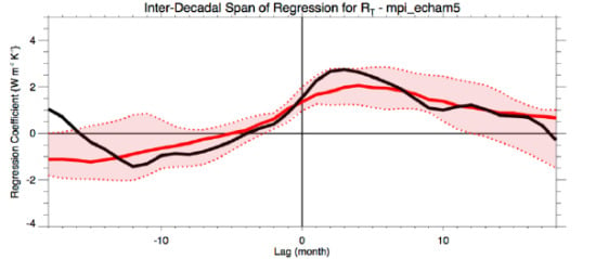
SB11 [8] suggest that the observational results are not replicated in models. The coupled climate models cover a hundred year period for the 20th century. The latter were detrended by SB11 but for the 20th century that is not necessary as the component of variance associated with the trend pales in comparison to that of ENSO. It is also possible to check results by using model control runs with no changes in forcing. However, rather than treat the model result as a single 100 year run, we can divide it into ten decade long samples of the same length as the observational record. In this way we can explore the decadal variability in the model framework and place error bars on the results, at least insofar as they pertain to natural variability. Figure 1 shows the results for the observations as in [8], but with the EBAF dataset, in black. Then we show results from two different models, one which does not replicate ENSO well (top) and one which does (second panel). In each panel we give the average result (red curve) for all 10 decades, plus the range of results that reflects the variations from one decade to the next. The MPI-Echam5 model replicates the observations very well. When all 14 model results from CMIP3 are included, the bottom panel results, showing the red curve similar to SB11 (their Figure 3) [8], but with a huge range (maximum to minimum), due both to the spread among models, and also the spread due to decadal variability. Hence many model results fall well within the range of uncertainties of the observations.

There are obvious differences among models. As noted by Dessler [10], it is important to sample all model results and not just select a few that may have certain specific deficiencies, as was done by SB11 [8]. Moreover, in examining the relationship of the regression’s strength among models to climate sensitivity we find a weak positive correlation—that is the models that do a better job of replicating the observed relationship are the higher sensitivity models, though it should also be remarked that the correlation is of marginally statistical significance, the precise value of which depends on the degrees of freedom attributed to the model ensemble. Consequently, bounding the response of models by selection of those with large and small sensitivities is inappropriate for these model-observation comparisons.

Because the exchange of heat between the ocean and atmosphere is a key part of the ENSO cycle [14], SB11’s simple model, which has no realistic ocean, no El Niño, and no hydrological cycle, and an inappropriate observational baseline, is unsuitable. Use of a reasonable heat capacity for the ocean is also crucial. Importantly, SB11 [8] treated non-radiative energy exchange between the ocean and atmosphere as a series of random numbers, which neglects the non-random variations of this energy flow associated with the ENSO cycle. During ENSO there is a major uptake of heat by the ocean during the La Niña phase and the heat is moved around and stored in the tropical western Pacific, setting the stage for the subsequent El Niño phase, during which the heat is redistributed across the tropical Pacific. The ocean cools as the atmosphere responds with weather patterns forced from high sea surface temperatures (SSTs) and this influences weather patterns world-wide. Ocean dynamics play a major role in this movement of heat, and atmosphere-ocean interaction is central to the ENSO cycle. None of those processes are included in the SB11 model and its relevance to nature is thus highly suspect.

Consequently, our results suggest that a range of model skills in replicating the regressions of SB11 exists, but rather than stratifying them by climate sensitivity as done without basis by SB11, one should stratify them by their ability to simulate ENSO. In Figure 1, the model that replicates the observations better has high sensitivity (3.4, which is the value in degrees Celsius for doubling carbon dioxide) while the other has low sensitivity (2.4). The net result is that some models agree within reasonable bounds with the observations, in contrast to the SB11 conclusions, but similar to Dessler (2011) [10] results. Moreover, the degree of model fidelity is not directly relevant to their climate sensitivity.

Figure 1. Slope of regression coefficients between monthly temperature anomalies and climate models using (upper) a model which does not accurately reproduce ENSO, (middle) a model which reproduces ENSO reasonably well, and (bottom) all CMIP3 models. Black lines are from observations, red lines are results averaged by decade, and red dashed lines indicate the range of model results.

Figure 1. Slope of regression coefficients between monthly temperature anomalies and climate models using (upper) a model which does not accurately reproduce ENSO, (middle) a model which reproduces ENSO reasonably well, and (bottom) all CMIP3 models. Black lines are from observations, red lines are results averaged by decade, and red dashed lines indicate the range of model results.

There is a lot more that could be done on this topic. Firstly, one could explore the systematic uncertainty associated with the different observational data sets and smoothing. Secondly, there is a need to explore the uncertainties in the regressions, a point touched on by Dessler [10]. Thirdly, the relationship with ENSO and the model ability to replicate ENSO, as well as its climate sensitivity could be explored further.

References

1. Gregory, J.M.; Ingram, W.J.; Palmer, M.A.; Jones, G.S.; Stott, P.A.; Thorpe, R.B.; Lowe, J.A.; Johns, T.C.; Williams, K.D. A new method for diagnosing radiative forcing and climate sensitivity. Geophys. Res. Lett. 2004, 31, L03205. [Google Scholar] [CrossRef]
2. Forster, P.M.F.; Gregory, J.M. The climate sensitivity and its components diagnosed from earth radiation budget data. J. Climate 2006, 19, 39–52. [Google Scholar] [CrossRef]
3. Spencer, R.W.; Braswell, W.D. On the diagnosis of radiative feedback in the presence of unknown radiative forcing. J. Geophys. Res. 2010, 115, D16109. [Google Scholar] [CrossRef]
4. Murphy, D.M.; Solomon, S.; Portmann, R.W.; Rosenlof, K.H.; Forster, P.M.; Wong, T. An observationally based energy balance for the earth since 1950. J. Geophys. Res. 2009, 114, D17107. [Google Scholar] [CrossRef]
5. Clement, A.C.; Burgman, R.; Norris, J.R. Observational and model evidence for positive low-level cloud feedback. Science 2009, 325, 460–464. [Google Scholar] [CrossRef] [PubMed]
6. Lindzen, R.S.; Choi, Y.-S. On the determination of climate feedbacks from erbe data. Geophys. Res. Lett. 2009, 36, L16705. [Google Scholar] [CrossRef]
7. Lindzen, R.S.; Choi, Y.S. On the observational determination of climate sensitivity and its implications. Asia Pacific J. Atmos. Sci. 2011, 47, 377–390. [Google Scholar] [CrossRef]
8. Spencer, R.W.; Braswell, W.D. On the misdiagnosis of surface temperature feedbacks from variations in earth’s radiant energy balance. Remote Sens. 2011, 3, 1603–1613. [Google Scholar] [CrossRef]
9. Dessler, A.E. A determination of the cloud feedback from climate variations over the past decade. Science 2010, 330, 1523–1527. [Google Scholar] [CrossRef] [PubMed]
10. Dessler, A.E. Cloud variations and the earth’s energy budget. Geophys. Res. Lett. 2011. [Google Scholar] [CrossRef]
11. Murphy, D.M. Constraining climate sensitivity with linear fits to outgoing radiation. Geophys. Res. Lett. 2010, 37, L09704. [Google Scholar] [CrossRef]
12. Chung, E.-S.; Soden, B.J.; Sohn, B.-J. Revisiting the determination of climate sensitivity from relationships between surface temperature and radiative fluxes. Geophys. Res. Lett. 2010, 37, L10703. [Google Scholar] [CrossRef]
13. Trenberth, K.E.; Fasullo, J.T.; O'Dell, C.; Wong, T. Relationships between tropical sea surface temperature and top-of-atmosphere radiation. Geophys. Res. Lett. 2010, 37, L03702. [Google Scholar] [CrossRef]
14. Trenberth, K.E. Changes in tropical clouds and radiation. Science 2002, 296, 2095. [Google Scholar] [CrossRef] [PubMed]
15. Wong, T.; Wielicki, B.A.; Lee, R.B.; Smith, G.L.; Bush, K.A.; Willis, J.K. Reexamination of the observed decadal variability of the earth radiation budget using altitude-corrected erbe/erbs nonscanner wfov data. J. Climate 2006, 19, 4028–4040. [Google Scholar] [CrossRef]
16. Fasullo, J.T.; Trenberth, K.E. The annual cycle of the energy budget. Part i: Global mean and land–ocean exchanges. J. Climate 2008, 21, 2297–2312. [Google Scholar] [CrossRef]
17. Trenberth, K.E.; Fasullo, J.T.; Kiehl, J. Earth’s global energy budget. Bull. Amer. Meteor. Soc. 2009, 90, 311–324. [Google Scholar] [CrossRef]
18. Trenberth, K. An imperative for climate change planning: Tracking earth's global energy. Current Opinion Environ. Sustain. 2009, 1, 19–27. [Google Scholar] [CrossRef]
19. Trenberth, K.E.; Fasullo, J.T. Tracking earth’s energy. Science 2010, 328, 316–317. [Google Scholar] [CrossRef] [PubMed]
20. Santer, B.D.; Mears, C.A.; Doutriaux, C.; Caldwell, P.M.; Gleckler, P.J.; Wigley, T.M.L.; Solomon, S.; Gillett, N.; Ivanova, D.P.; Karl, T.R.; et al. Separating signal and noise in atmospheric temperature changes: The importance of timescale. J. Geophys. Res. 2011. [Google Scholar] [CrossRef]
21. Easterling, D.R.; Wehner, M.F. Is the climate warming or cooling? Geophys. Res. Lett. 2009, 36, L08706. [Google Scholar] [CrossRef]
22. Palmer, M.D.; McNeall, D.J.; Dunstone, N.J. Importance of the deep ocean for estimating decadal changes in earth’s radiation balance. Geophys. Res. Lett. 2011, 38, L13707. [Google Scholar] [CrossRef]
23. Katsman, C.A.; van Oldenborgh, G.J. Tracing the upper ocean’s “Missing heat”. Geophys. Res. Lett. 2011, 38, L14610. [Google Scholar] [CrossRef]
24. Meehl, G.A.; Arblaster, J.; Fasullo, J.; Hu, A.; Trenberth, K. Model-based evidence of deep ocean heat uptake during surface temperature hiatus periods. Nature Climate Change 2011, 1. [Google Scholar] [CrossRef]
25. NASA. CERES EBAF Data Sets. Available online: http://eosweb.larc.nasa.gov/PRODOCS/ceres/level4_ebaf_table.html (accessed on 8 September 2011).