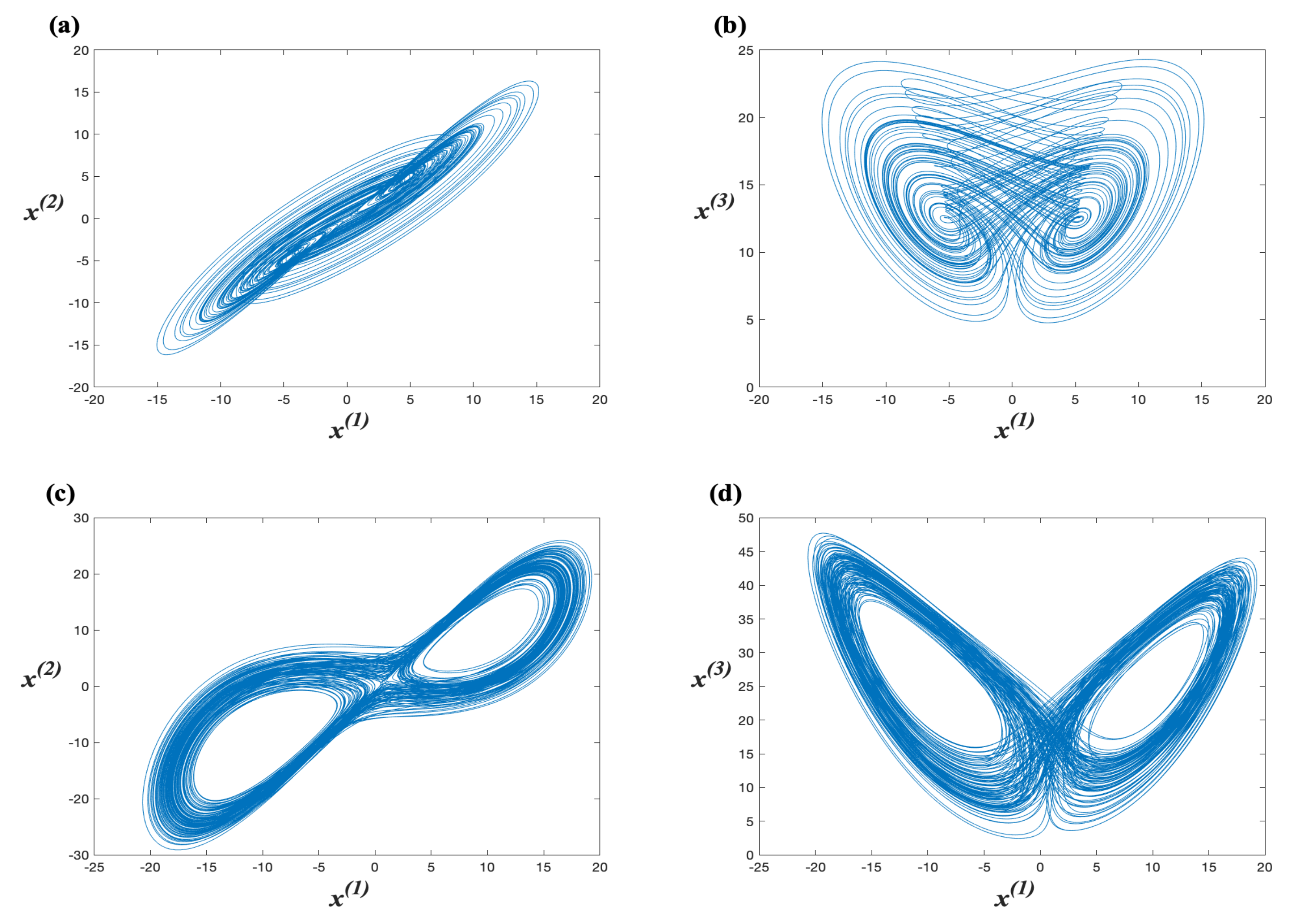
Figure 1.
The hyperchaotic attractors of Lorenz’s system projected on the planes (a) and (b) . The hyperchaotic attractors of Chen’s system projected on the planes (c) and (d) .
Figure 1.
The hyperchaotic attractors of Lorenz’s system projected on the planes (a) and (b) . The hyperchaotic attractors of Chen’s system projected on the planes (c) and (d) .
Figure 2.
A standard ZigZag transform scheme.
Figure 2.
A standard ZigZag transform scheme.
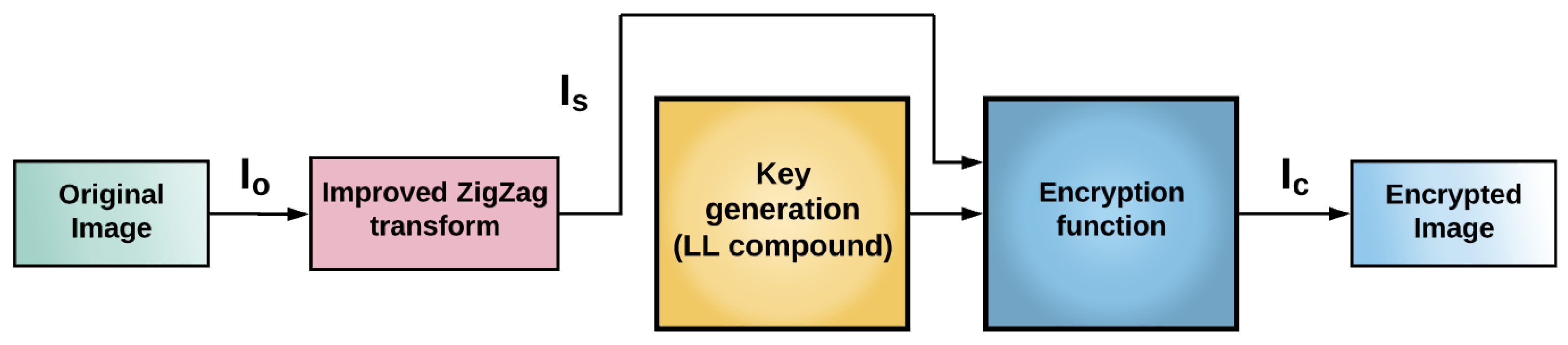
Figure 3.
Schematic diagram of the encryption system proposed by Xingyuan et al. [
3]. At first, an improved ZigZag transform is applied to the original image (
) resulting in an image
. The latter image and the generated key
K are the input to the encryption function obtaining an encrypted image
.
Figure 3.
Schematic diagram of the encryption system proposed by Xingyuan et al. [
3]. At first, an improved ZigZag transform is applied to the original image (
) resulting in an image
. The latter image and the generated key
K are the input to the encryption function obtaining an encrypted image
.
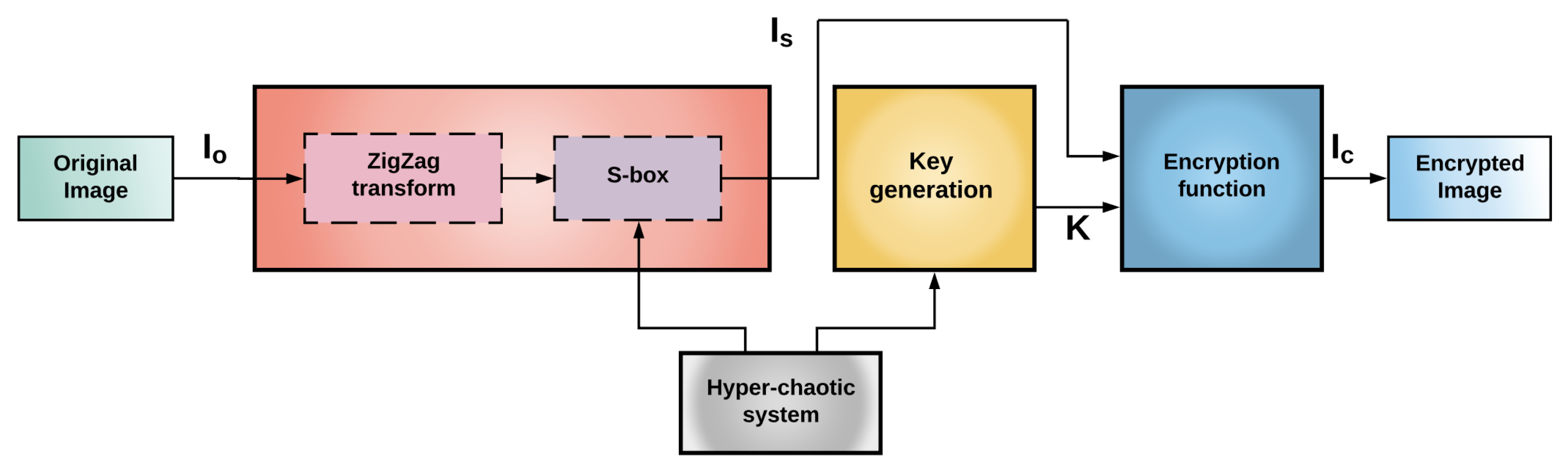
Figure 4.
Block diagram of our proposed encryption system. An image is obtained after the standard ZigZag, and the S-box procedures are applied to the original image . The image and the generated key K are the input to the encryption function resulting in an encrypted image .
Figure 4.
Block diagram of our proposed encryption system. An image is obtained after the standard ZigZag, and the S-box procedures are applied to the original image . The image and the generated key K are the input to the encryption function resulting in an encrypted image .
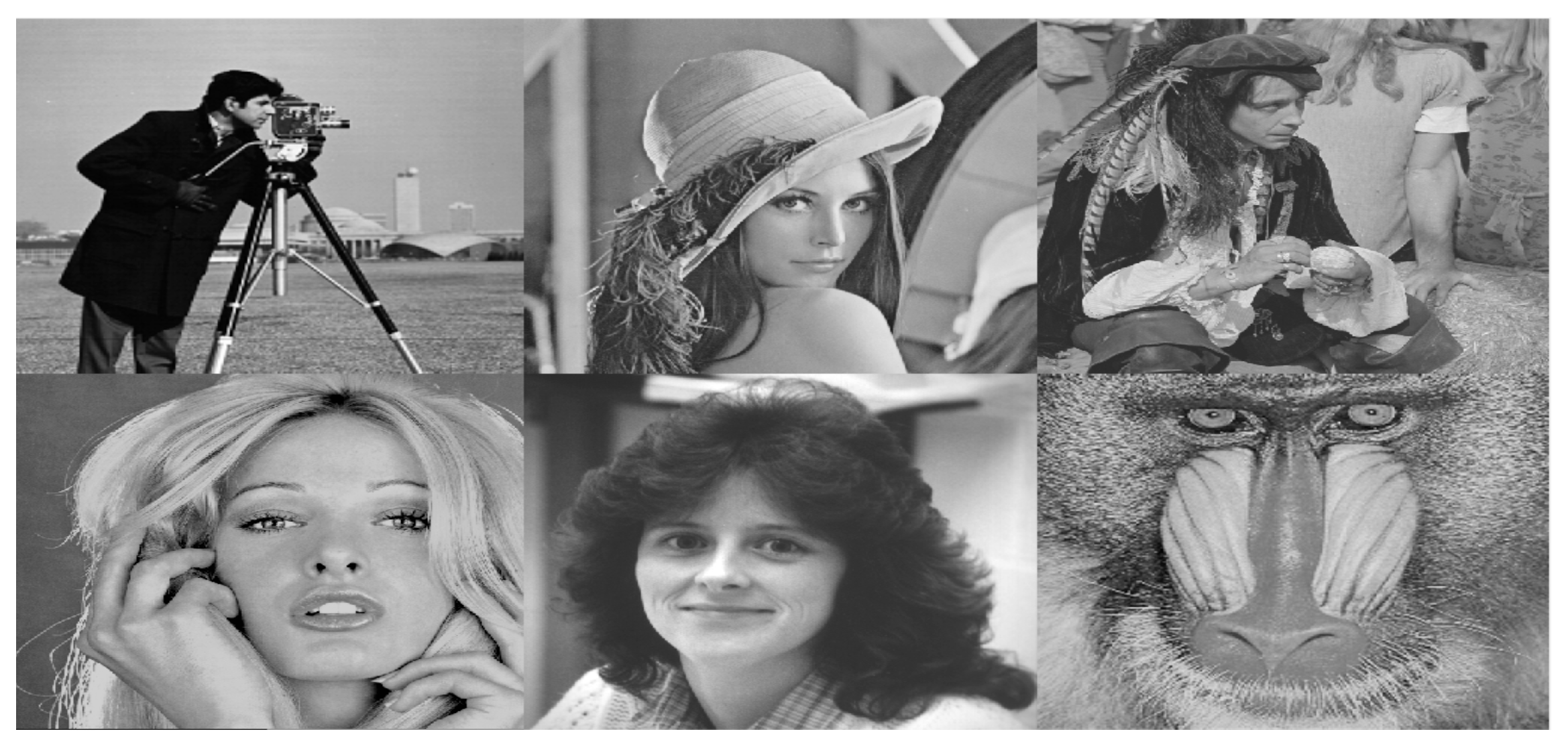
Figure 5.
The image dataset considered in this work. Original images () of size , each image is numbered 1 to 6 from left to right and top to bottom.
Figure 5.
The image dataset considered in this work. Original images () of size , each image is numbered 1 to 6 from left to right and top to bottom.
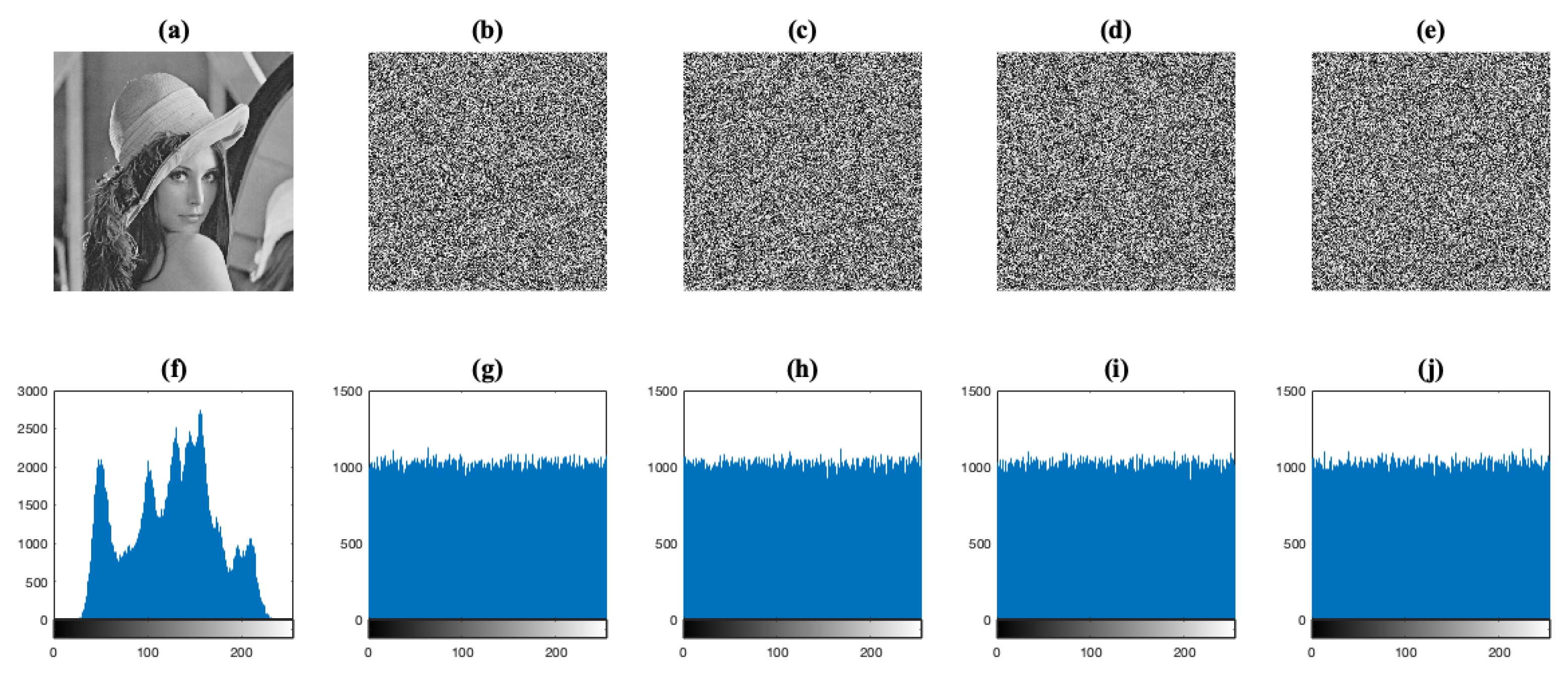
Figure 6.
Histogram analysis for the Lena test image. (a) The plain image . (b–e) The images considering the image encryption systems , , , and , respectively. (f–j) The corresponding histograms of images (a–e).
Figure 6.
Histogram analysis for the Lena test image. (a) The plain image . (b–e) The images considering the image encryption systems , , , and , respectively. (f–j) The corresponding histograms of images (a–e).
Figure 7.
Histogram analysis for the Lena test image. (a) The plain image . (b–e) The encrypted images with the image encryption systems , , , and , respectively. (f–j) The corresponding histograms of images (a–e).
Figure 7.
Histogram analysis for the Lena test image. (a) The plain image . (b–e) The encrypted images with the image encryption systems , , , and , respectively. (f–j) The corresponding histograms of images (a–e).
Figure 8.
Correlation plot of two adjacent pixels at the horizontal direction for (a) the Lena test image and (b–e) the images considering the image encryption systems , , , and , respectively.
Figure 8.
Correlation plot of two adjacent pixels at the horizontal direction for (a) the Lena test image and (b–e) the images considering the image encryption systems , , , and , respectively.
Figure 9.
Correlation plot of two adjacent pixels at the horizontal direction for (a) the Lena test image and (b–e) the encrypted images with the image encryption systems , , , and , respectively.
Figure 9.
Correlation plot of two adjacent pixels at the horizontal direction for (a) the Lena test image and (b–e) the encrypted images with the image encryption systems , , , and , respectively.
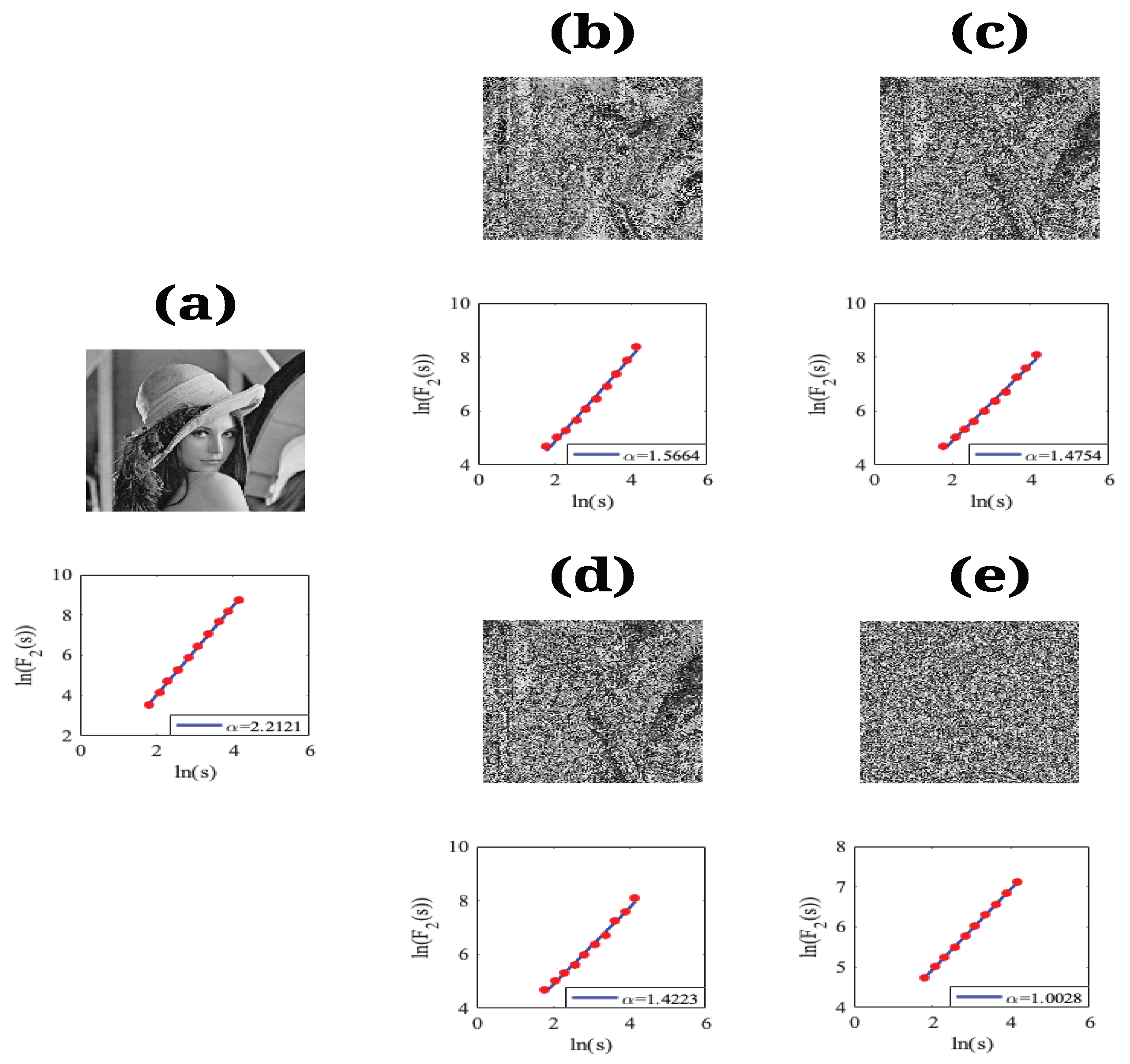
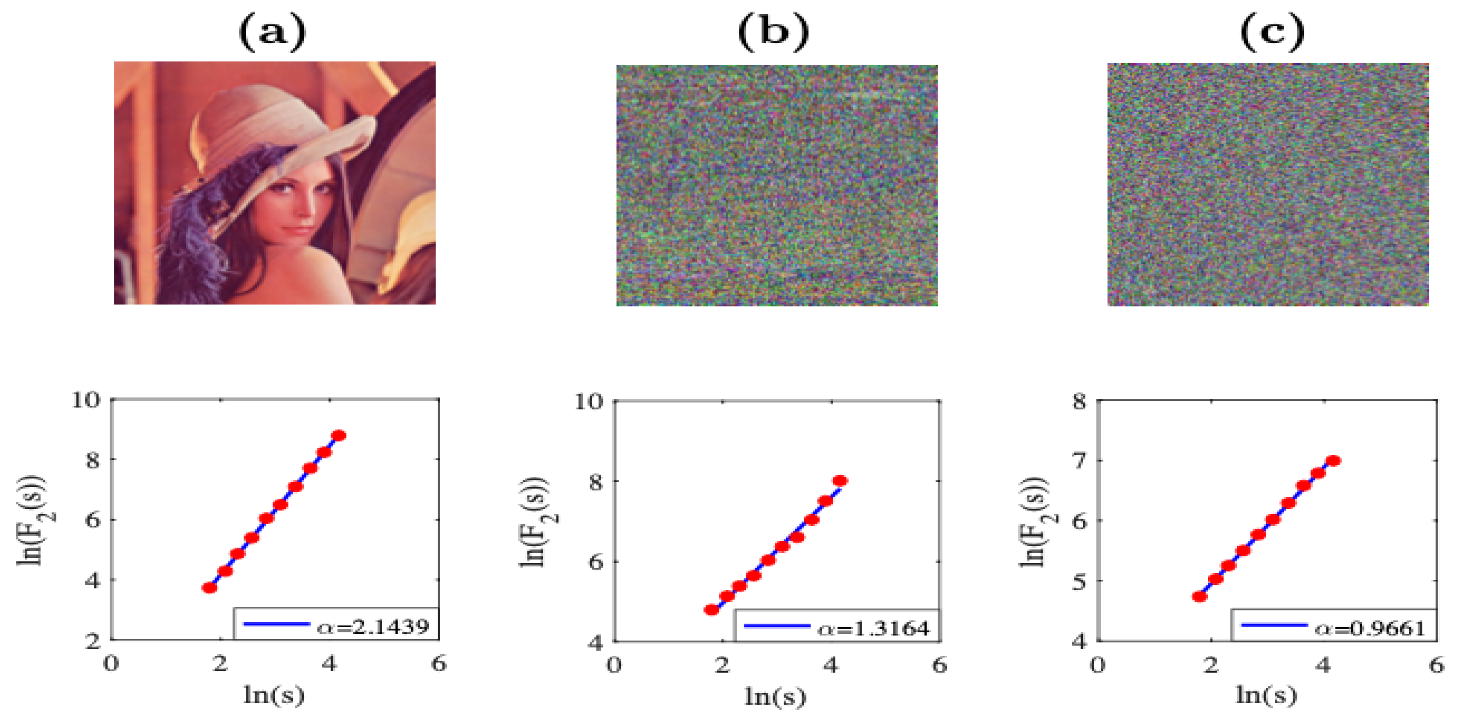
Figure 10.
(a) The Lena test image and its respective scaling analysis. (b,c) The and images with their respective scaling analysis, where the S-box of the system is considered in the scrambling stage. (d,e) The and images with their respective scaling analysis, where the complete scrambling stage in the system is considered.
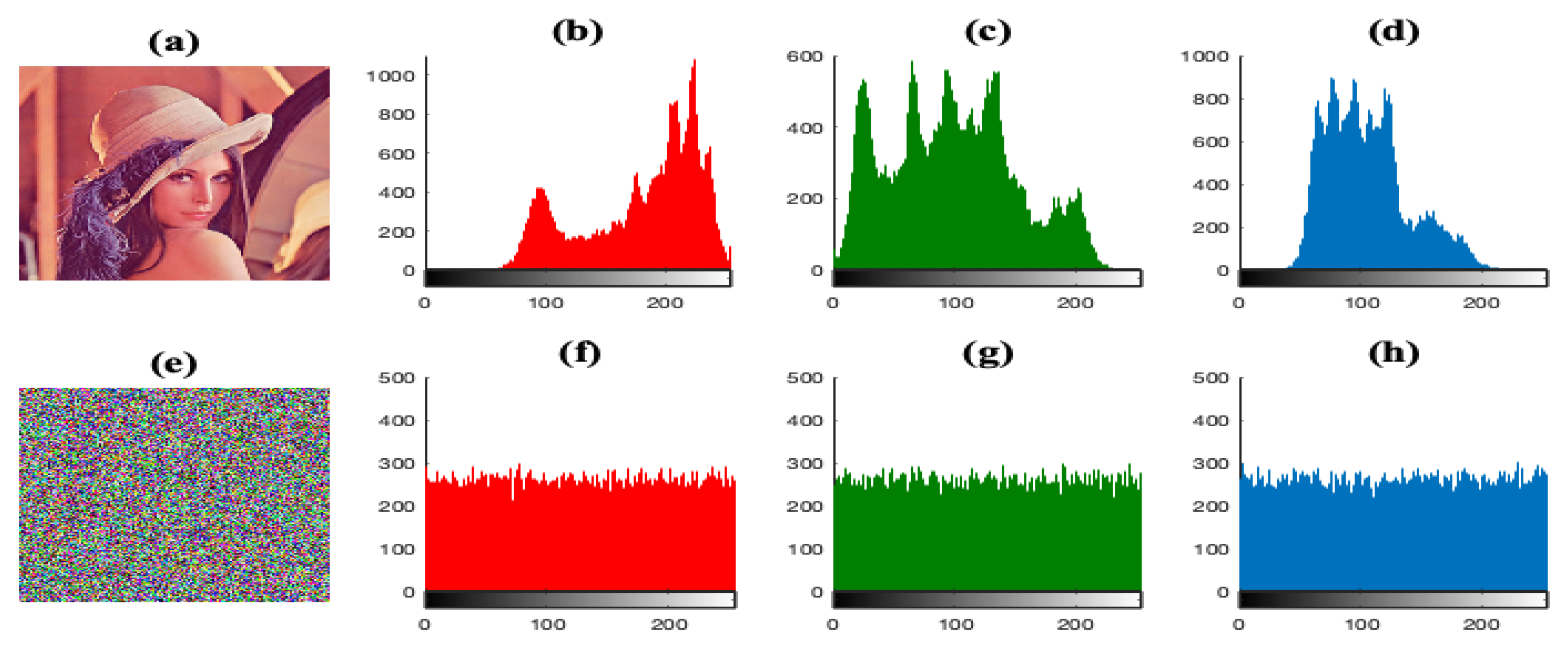
Figure 11.
Histogram analysis for the color Lena test image. (a) The plain-image . (b–d) Histograms for red, green and blue channels, respectively. (e) The encrypted Lena image considering the image encryption system . (f–h) The corresponding histograms for red, green and blue channels of the encrypted image (e).
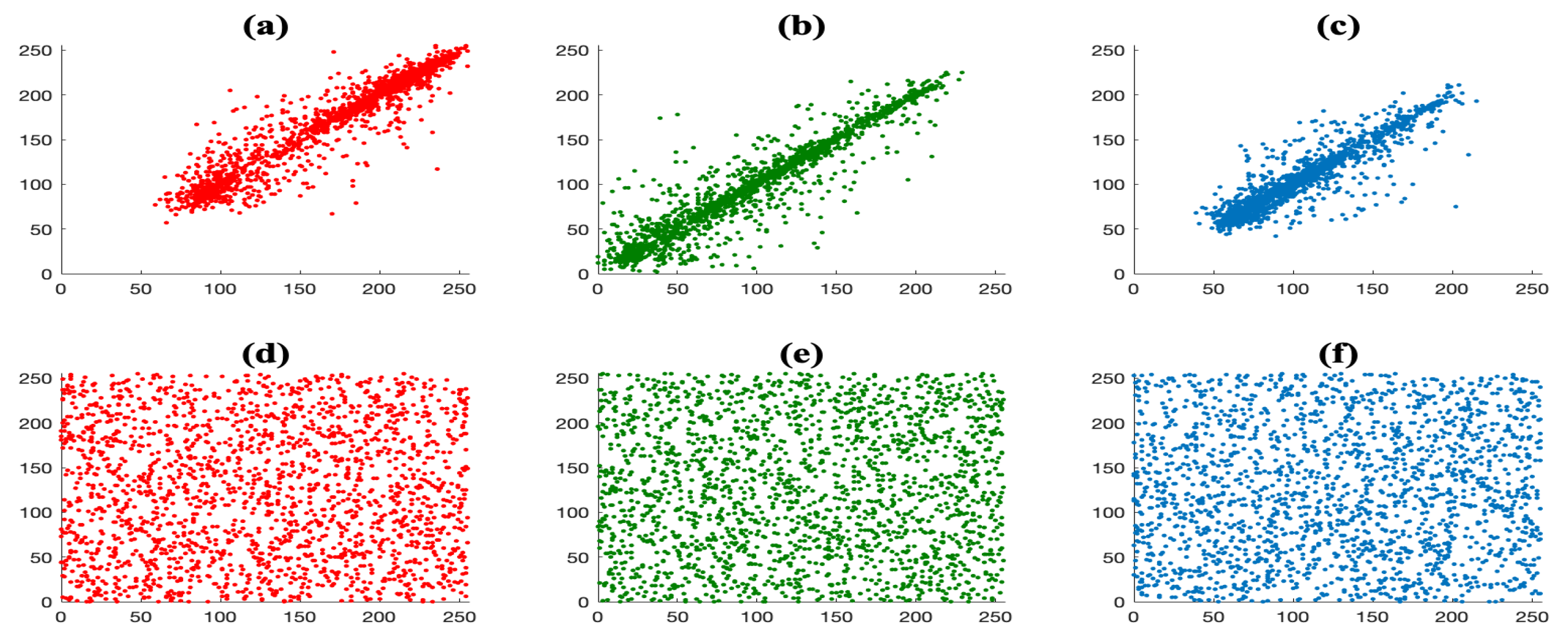
Figure 12.
Correlation plot of two adjacent pixels for the color Lena test image (top) and its encrypted version (bottom), using , at the horizontal (first column), vertical (second column), and diagonal (third column) direction.
Figure 12.
Correlation plot of two adjacent pixels for the color Lena test image (top) and its encrypted version (bottom), using , at the horizontal (first column), vertical (second column), and diagonal (third column) direction.
Figure 13.
(a) The color Lena test image, (b) the , and (c) images, with their respective scaling analysis when the complete scrambling stage in the system is considered.
Figure 13.
(a) The color Lena test image, (b) the , and (c) images, with their respective scaling analysis when the complete scrambling stage in the system is considered.
Table 1.
p-values of the hypothesis test for the encrypted images.
Table 1.
p-values of the hypothesis test for the encrypted images.
| Image | p-Values |
|---|
| | | |
|---|
| 1 | 0.3187 | 0.1375 | 0.7522 | 0.3187 |
| 2 | 0.2523 | 0.2315 | 0.5076 | 0.3419 |
| 3 | 0.0615 | 0.7384 | 0.0052 | 0.1463 |
| 4 | 0.6579 | 0.2443 | 0.9445 | 0.4398 |
| 5 | 0.3718 | 0.5787 | 0.5150 | 0.3920 |
| 6 | 0.7848 | 0.9676 | 0.2627 | 0.8596 |
Table 2.
Correlation coefficients between adjacent pixels of plain images and their images considering the standard and improved ZigZag transformation in the scrambling stage.
Table 2.
Correlation coefficients between adjacent pixels of plain images and their images considering the standard and improved ZigZag transformation in the scrambling stage.
| Correlation Coefficients |
|---|
|
Image
| |
Standard ZigZag Operation
|
Improved ZigZag Operation
|
|---|
|
h
|
v
|
d
|
h
|
v
|
d
|
h
|
v
|
d
|
|---|
| 1 | 0.9838 | 0.9858 | 0.9743 | 0.9747 | −0.0549 | −0.0520 | 0.9688 | 0.5624 | 0.5627 |
| 2 | 0.9848 | 0.9895 | 0.9798 | 0.9670 | 0.0328 | 0.0377 | 0.9647 | 0.3275 | 0.3320 |
| 3 | 0.9710 | 0.9791 | 0.9605 | 0.9412 | 0.1039 | 0.0979 | 0.9387 | 0.3542 | 0.3603 |
| 4 | 0.9727 | 0.9752 | 0.9629 | 0.9343 | 0.2256 | 0.2149 | 0.9319 | 0.3555 | 0.3564 |
| 5 | 0.9942 | 0.9959 | 0.9923 | 0.9937 | 0.0497 | 0.0495 | 0.9862 | 0.4799 | 0.4798 |
| 6 | 0.9477 | 0.9317 | 0.9078 | 0.8662 | 0.1003 | 0.1221 | 0.8579 | 0.3117 | 0.2972 |
Table 3.
Correlation coefficients between adjacent pixels of plain images and their images obtained with the S-box of the , and systems in the scrambling stage.
Table 3.
Correlation coefficients between adjacent pixels of plain images and their images obtained with the S-box of the , and systems in the scrambling stage.
| Correlation Coefficients |
|---|
|
Image
| | | |
|---|
|
h
|
v
|
d
|
h
|
v
|
d
|
h
|
v
|
d
|
|---|
| 1 | 0.2330 | 0.2311 | 0.1852 | 0.3580 | 0.3275 | 0.2483 | 0.1984 | 0.2494 | 0.1758 |
| 2 | 0.1442 | 0.1348 | 0.0636 | 0.1497 | 0.1945 | 0.1442 | 0.0862 | 0.1019 | 0.0618 |
| 3 | 0.0585 | 0.0917 | 0.0531 | 0.1387 | 0.1353 | 0.0740 | 0.0871 | 0.0596 | 0.0426 |
| 4 | 0.1095 | 0.1383 | 0.0748 | 0.1709 | 0.1870 | 0.1522 | 0.0687 | 0.0532 | 0.0418 |
| 5 | 0.1104 | 0.1384 | 0.1123 | 0.2002 | 0.2715 | 0.1695 | 0.1470 | 0.1234 | 0.0676 |
| 6 | 0.0742 | 0.0462 | 0.0474 | 0.0889 | 0.1113 | 0.0707 | 0.0280 | 0.0489 | 0.0444 |
Table 4.
Correlation coefficients between adjacent pixels of the images considering the and systems.
Table 4.
Correlation coefficients between adjacent pixels of the images considering the and systems.
| Correlation Coefficients |
|---|
|
Image
| | |
|---|
|
h
|
v
|
d
|
h
|
v
|
d
|
|---|
| 1 | 0.0153 | −0.0309 | 0.0014 | 0.2095 | 0.2165 | 0.1432 |
| 2 | 0.0188 | 0.0297 | −0.0003 | 0.0122 | 0.0120 | 0.0979 |
| 3 | 0.0109 | −0.0025 | 0.0004 | 0.0752 | 0.0825 | 0.0513 |
| 4 | 0.0016 | 0.0588 | 0.0130 | 0.0100 | 0.0701 | 0.0980 |
| 5 | 0.0065 | 0.0152 | 0.0182 | 0.0143 | 0.0012 | 0.0092 |
| 6 | −0.0001 | −0.0016 | −0.0661 | 0.0031 | 0.0032 | 0.0023 |
Table 5.
Correlation coefficients between adjacent pixels of the images considering the and systems.
Table 5.
Correlation coefficients between adjacent pixels of the images considering the and systems.
| Correlation Coefficients |
|---|
|
Image
| | |
|---|
|
h
|
v
|
d
|
h
|
v
|
d
|
|---|
| 1 | 0.3499 | 0.3146 | 0.2588 | 0.2094 | 0.2248 | 0.1455 |
| 2 | 0.1608 | 0.1931 | 0.1327 | 0.0822 | 0.0874 | 0.0887 |
| 3 | 0.0143 | 0.0134 | 0.0129 | 0.0952 | 0.0977 | 0.0543 |
| 4 | 0.0162 | 0.0212 | 0.0151 | 0.0726 | 0.0517 | 0.0516 |
| 5 | 0.0021 | 0.0023 | 0.0019 | 0.1134 | 0.1338 | 0.1156 |
| 6 | 0.0812 | 0.0043 | 0.0690 | 0.0578 | 0.0542 | 0.0158 |
Table 6.
Correlation coefficients between adjacent pixels of the images considering the and systems.
Table 6.
Correlation coefficients between adjacent pixels of the images considering the and systems.
| Correlation Coefficients |
|---|
|
Image
| | |
|---|
|
h
|
v
|
d
|
h
|
v
|
d
|
|---|
| 1 | 0.0690 | 0.0034 | 0.0261 | 0.0029 | −0.0019 | −0.0126 |
| 2 | 0.0727 | −0.0198 | −0.484 | 0.0029 | −0.0019 | −0.0126 |
| 3 | −0.0087 | −0.0078 | 0.0239 | 0.0698 | 0.0729 | 0.0792 |
| 4 | −0.0035 | 0.0096 | −0.0190 | 0.0117 | −0.0225 | 0.0156 |
| 5 | 0.0511 | −0.050 | −0.0039 | 0.0183 | 0.0092 | −0.0168 |
| 6 | −0.0058 | −0.0050 | 0.0452 | 0.0044 | 0.0211 | 0.0159 |
Table 7.
Correlation coefficients between adjacent pixels of the images considering the and systems.
Table 7.
Correlation coefficients between adjacent pixels of the images considering the and systems.
| Correlation Coefficients |
|---|
|
Image
| | |
|---|
|
h
|
v
|
d
|
h
|
v
|
d
|
|---|
| 1 | 0.0036 | 0.0048 | 0.0152 | −0.0050 | 0.0006 | 0.0015 |
| 2 | 0.0036 | 0.0048 | 0.0152 | −0.0156 | −0.0115 | 0.0189 |
| 3 | 0.1399 | 0.1293 | 0.0976 | 0.0261 | −0.0014 | 0.0288 |
| 4 | 0.0068 | −0.0062 | −0.0018 | −0.0018 | 0.0250 | −0.0057 |
| 5 | −0.0193 | −0.0031 | −0.0103 | 0.0178 | −0.0139 | 0.0061 |
| 6 | 0.0015 | 0.0016 | −0.0109 | −0.0028 | 0.0104 | −0.0143 |
Table 8.
Expected NPCR (%) and UACI (%) values for some cases when the standard ZigZag (S-ZZ) and improved ZigZag (I-ZZ) transformation are applied to images in the scrambling and encryption stages.
Table 8.
Expected NPCR (%) and UACI (%) values for some cases when the standard ZigZag (S-ZZ) and improved ZigZag (I-ZZ) transformation are applied to images in the scrambling and encryption stages.
| Image → | | |
|---|
| System↓ | | | | | | |
| with I-ZZ | 97.5023 | 32.1023 | 32.9938 | 98.1233 | 33.3312 | 33.6310 |
| with S-box | 97.9002 | 31.1025 | 31.9533 | 98.2313 | 33.1133 | 33.7521 |
| with S-ZZ and S-box | 99.3312 | 33.2815 | 33.5731 | 99.6135 | 33.3328 | 33.5451 |
Table 9.
NPCR (%) and UACI (%) values when the standard ZigZag (S-ZZ) and improved ZigZag (I-ZZ) transformation are applied to images in the scrambling and encryption stages.
Table 9.
NPCR (%) and UACI (%) values when the standard ZigZag (S-ZZ) and improved ZigZag (I-ZZ) transformation are applied to images in the scrambling and encryption stages.
| | | |
|---|
|
Image
|
S-ZZ
|
I-ZZ
|
S-ZZ
|
I-ZZ
|
|---|
|
NPCR
|
UACI
|
NPCR
|
UACI
|
NPCR
|
UACI
|
NPCR
|
UACI
|
|---|
| 1 | 97.5672 | 33.3830 | 97.0600 | 31.2290 | 98.6108 | 33.3330 | 97.0137 | 32.2630 |
| 2 | 97.6622 | 32.9965 | 98.1769 | 31.9929 | 98.7830 | 32.2187 | 97.1992 | 32.5631 |
| 3 | 97.4531 | 32.1238 | 97.9945 | 31.9995 | 98.8612 | 33.0953 | 98.0945 | 32.9752 |
| 4 | 97.9954 | 31.9549 | 97.4301 | 31.9437 | 98.0167 | 33.3316 | 98.9012 | 33.2139 |
| 5 | 97.9128 | 32.9981 | 98.1956 | 32.2190 | 98.5621 | 33.4319 | 98.1605 | 33.4691 |
| 6 | 97.4182 | 32.4794 | 97.3981 | 32.2964 | 98.1598 | 33.4189 | 98.9158 | 33.4498 |
| Pass | 5 | 5 | 6 | 5 | 5 | 4 | 5 | 5 |
| Mean | 97.6681 | 32.6559 | 97.7092 | 31.9466 | 98.4989 | 33.1377 | 98.0474 | 32.9940 |
| Std | 0.0571 | 0.3134 | 0.2265 | 0.1432 | 0.1151 | 0.2175 | 0.6572 | 0.2404 |
Table 10.
NPCR (%) and UACI (%) values considering and images when the S-box of the , and systems are applied to images in the scrambling stage.
Table 10.
NPCR (%) and UACI (%) values considering and images when the S-box of the , and systems are applied to images in the scrambling stage.
| | |
|---|
|
Image
| | | |
|---|
|
NPCR
|
UACI
|
NPCR
|
UACI
|
NPCR
|
UACI
|
|---|
| 1 | 97.9124 | 31.9252 | 97.0467 | 32.3768 | 96.9961 | 32.4314 |
| 2 | 98.0496 | 31.2461 | 97.0459 | 32.4592 | 97.1198 | 32.9832 |
| 3 | 97.9047 | 31.9010 | 97.8830 | 32.1674 | 97.9179 | 32.9174 |
| 4 | 98.3955 | 31.2061 | 97.7819 | 31.0194 | 97.5991 | 31.0173 |
| 5 | 97.8728 | 31.2187 | 97.1298 | 32.2109 | 97.0652 | 32.2487 |
| 6 | 98.1807 | 31.2205 | 97.9612 | 31.0175 | 97.1921 | 31.0147 |
| Pass | 6 | 6 | 5 | 4 | 5 | 4 |
| Mean | 98.0526 | 31.4529 | 97.4747 | 31.8752 | 97.3150 | 32.1021 |
| Std | 0.0415 | 0.1272 | 0.1967 | 0.4517 | 0.1323 | 0.7860 |
Table 11.
NPCR (%) and UACI (%) values considering the and images when the S-box of the , , and systems are applied to images in the scrambling stage.
Table 11.
NPCR (%) and UACI (%) values considering the and images when the S-box of the , , and systems are applied to images in the scrambling stage.
| | |
|---|
|
Image
| | | |
|---|
|
NPCR
|
UACI
|
NPCR
|
UACI
|
NPCR
|
UACI
|
|---|
| 1 | 99.0783 | 33.1338 | 98.2983 | 32.9927 | 99.0485 | 32.9832 |
| 2 | 98.9916 | 33.1859 | 98.9630 | 32.7950 | 99.7391 | 33.3861 |
| 3 | 99.5842 | 33.4997 | 99.4598 | 33.0937 | 98.9937 | 33.2487 |
| 4 | 98.4461 | 33.2643 | 99.5293 | 33.2197 | 98.3671 | 33.2201 |
| 5 | 98.1845 | 33.3432 | 98.9932 | 33.3141 | 98.6825 | 33.2826 |
| 6 | 98.2901 | 32.3379 | 98.2017 | 33.3357 | 98.9951 | 33.3261 |
| Pass | 5 | 6 | 5 | 5 | 5 | 5 |
| Mean | 98.7624 | 33.1274 | 98.9075 | 33.1251 | 98.9710 | 33.2411 |
| Std | 0.2969 | 0.1661 | 0.3142 | 0.0433 | 0.2090 | 0.0193 |
Table 12.
NPCR (%) and UACI (%) values considering and images with the systems in the scrambling stage with two operations.
Table 12.
NPCR (%) and UACI (%) values considering and images with the systems in the scrambling stage with two operations.
| | Scrambling Block |
|---|
|
Image
|
NPCR
|
UACI
|
|---|
| | | | | | | |
|---|
| 1 | 98.9993 | 99.5691 | 99.6881 | 99.1727 | 33.4662 | 33.2931 | 33.4621 | 33.4638 |
| 2 | 99.3956 | 99.6142 | 99.6129 | 99.4328 | 33.3687 | 33.4637 | 33.4674 | 33.4643 |
| 3 | 99.2137 | 99.6344 | 99.6017 | 99.3449 | 33.4431 | 33.4631 | 33.4538 | 33.4459 |
| 4 | 99.4429 | 99.6147 | 99.6045 | 99.6327 | 33.4537 | 33.4638 | 33.4625 | 33.4452 |
| 5 | 99.4414 | 99.6134 | 99.6827 | 99.6157 | 33.4238 | 33.4545 | 33.4545 | 33.4637 |
| 6 | 99.4215 | 99.6135 | 99.6122 | 99.6020 | 33.4632 | 33.4623 | 33.4632 | 33.4628 |
| Pass | 6 | 6 | 6 | 6 | 6 | 6 | 6 | 6 |
| Mean | 99.3190 | 99.6098 | 99.6336 | 99.4667 | 33.4364 | 33.4334 | 33.4605 | 33.4576 |
| Std | 0.0320 | 0.0004 | 0.0016 | 0.0340 | 0.0013 | 0.0047 | 0.0025 | 0.0084 |
Table 13.
NPCR (%) and UACI (%) values considering and images with the systems when two operations are considered in the scrambling stage.
Table 13.
NPCR (%) and UACI (%) values considering and images with the systems when two operations are considered in the scrambling stage.
| | Encryption Block |
|---|
|
Image
|
NPCR
|
UACI
|
|---|
| | | | | | | |
|---|
| 1 | 99.6112 | 99.6226 | 99.9083 | 99.6028 | 33.4926 | 33.4748 | 33.4843 | 33.4838 |
| 2 | 99.5932 | 99.6633 | 99.6825 | 99.6033 | 33.4693 | 33.4683 | 33.4683 | 33.4782 |
| 3 | 99.6135 | 99.6383 | 99.6838 | 99.6139 | 33.4739 | 33.4874 | 33.4635 | 33.4632 |
| 4 | 99.6133 | 99.6253 | 99.6335 | 99.6873 | 33.4843 | 33.4724 | 33.4639 | 33.4639 |
| 5 | 99.6332 | 99.7823 | 99.7172 | 99.7643 | 33.4934 | 33.4891 | 33.4718 | 33.4763 |
| 6 | 99.6123 | 99.6298 | 99.6382 | 99.6273 | 33.4793 | 33.4636 | 33.4693 | 33.4697 |
| Pass | 6 | 6 | 6 | 6 | 6 | 6 | 6 | 6 |
| Mean | 99.6127 | 99.6552 | 99.7105 | 99.6498 | 33.4821 | 33.4759 | 33.4701 | 33.4725 |
| Std | 0.0016 | 0.0039 | 0.0103 | 0.0041 | 0.0937 | 0.0012 | 0.0054 | 0.0063 |
Table 14.
The comparison of information entropies for the and images when the standard ZigZag (S-ZZ) and improved ZigZag (I-ZZ) transformation are applied to images in the scrambling stage.
Table 14.
The comparison of information entropies for the and images when the standard ZigZag (S-ZZ) and improved ZigZag (I-ZZ) transformation are applied to images in the scrambling stage.
| Entropy |
|---|
|
Image
| | | |
|---|
|
S-ZZ
|
I-ZZ
|
S-ZZ
|
I-ZZ
|
|---|
| 1 | 7.0478 | 7.0479 | 7.0477 | 7.9989 | 7.9980 |
| 2 | 7.4451 | 7.4452 | 7.4449 | 7.9977 | 7.9975 |
| 3 | 7.2367 | 7.2367 | 7.2368 | 7.9966 | 7.9964 |
| 4 | 6.9542 | 6.9544 | 6.9541 | 7.9965 | 7.9953 |
| 5 | 7.2757 | 7.2760 | 7.2765 | 7.9974 | 7.9983 |
| 6 | 7.2925 | 7.2930 | 7.2921 | 7.9990 | 7.9990 |
Table 15.
The comparison of information entropies for the and images when the S-box of the , , and systems is applied to images in the scrambling stage.
Table 15.
The comparison of information entropies for the and images when the S-box of the , , and systems is applied to images in the scrambling stage.
| Entropy |
|---|
|
Image
| | |
|---|
| | | | | |
|---|
| 1 | 7.0477 | 7.0480 | 7.0478 | 7.9980 | 7.9984 | 7.9983 |
| 2 | 7.4459 | 7.4465 | 7.4460 | 7.9986 | 7.9984 | 7.9988 |
| 3 | 7.2370 | 7.2374 | 7.2367 | 7.9990 | 7.9991 | 7.9991 |
| 4 | 6.9550 | 6.9548 | 6.9545 | 7.9991 | 7.9991 | 7.9991 |
| 5 | 7.2740 | 7.2743 | 7.2740 | 7.9983 | 7.9987 | 7.9980 |
| 6 | 7.2935 | 7.2930 | 7.2929 | 7.9991 | 7.9991 | 7.9989 |
Table 16.
The comparison of information entropies for the and images when the complete scrambling stage is applied to images .
Table 16.
The comparison of information entropies for the and images when the complete scrambling stage is applied to images .
| | Entropy |
|---|
|
Image
| | |
|---|
| | | | | | | |
|---|
| 1 | 7.0478 | 7.0477 | 7.0477 | 7.0464 | 7.9993 | 7.9993 | 7.9993 | 7.9993 |
| 2 | 7.4451 | 7.4451 | 7.4451 | 7.4451 | 7.9993 | 7.9993 | 7.9993 | 7.9993 |
| 3 | 7.2367 | 7.2367 | 7.2367 | 7.2367 | 7.9992 | 7.9993 | 7.9994 | 7.9993 |
| 4 | 6.9542 | 6.9542 | 6.9542 | 6.9542 | 7.9993 | 7.9993 | 7.9993 | 7.9994 |
| 5 | 7.2757 | 7.2737 | 7.2737 | 7.2757 | 7.9992 | 7.9992 | 7.9993 | 7.9994 |
| 6 | 7.2925 | 7.2925 | 7.2925 | 7.2925 | 7.9993 | 7.9993 | 7.9993 | 7.9994 |
Table 17.
PNSR values in considering the complete scrambling.
Table 17.
PNSR values in considering the complete scrambling.
| | PSNR Values |
|---|
|
Image
| | |
|---|
| | | | | | | |
|---|
| 1 | 13.1462 | 15.7231 | 13.0126 | 13.0480 | 7.8623 | 7.4127 | 7.9827 | 7.4568 |
| 2 | 12.1596 | 13.0690 | 12.5056 | 12.1596 | 8.3917 | 8.4818 | 8.6578 | 8.2682 |
| 3 | 12.4326 | 13.2715 | 13.2670 | 11.2021 | 8.8176 | 8.8086 | 8.8526 | 8.8264 |
| 4 | 13.3398 | 12.4504 | 12.4812 | 13.5120 | 7.9042 | 7.9827 | 7.8129 | 7.6559 |
| 5 | 11.3313 | 11.4401 | 11.0419 | 11.4757 | 8.9271 | 8.8597 | 8.8045 | 8.7528 |
| 6 | 13.8149 | 13.7376 | 13.6122 | 13.3356 | 9.4522 | 9.4782 | 9.4529 | 9.2740 |
Table 18.
The comparison of information of the scaling exponents obtained from applying the 2D-DFA scheme to the , , and images, when the standard ZigZag (S-ZZ) and improved ZigZag (I-ZZ) transformation are applied to images in the scrambling stage.
Table 18.
The comparison of information of the scaling exponents obtained from applying the 2D-DFA scheme to the , , and images, when the standard ZigZag (S-ZZ) and improved ZigZag (I-ZZ) transformation are applied to images in the scrambling stage.
| | Exponents |
|---|
|
Image
| | | |
|---|
|
S-ZZ
|
I-ZZ
|
S-ZZ
|
I-ZZ
|
|---|
| 1 | 2.1990 | 1.9504 | 1.7666 | 1.8956 | 1.8603 |
| 2 | 2.2121 | 1.8130 | 1.6232 | 1.8845 | 1.8556 |
| 3 | 2.2851 | 1.8130 | 1.6389 | 1.6329 | 1.8594 |
| 4 | 2.1970 | 1.8808 | 1.5421 | 1.5421 | 1.8063 |
| 5 | 2.5659 | 1.8495 | 1.8152 | 1.7881 | 1.6562 |
| 6 | 1.9218 | 1.7336 | 1.8091 | 1.9323 | 1.8921 |
Table 19.
The comparison of information of the scaling exponents obtained from applying the 2D-DFA scheme to the and images, when the S-box of the , , and systems is applied to images in the scrambling stage.
Table 19.
The comparison of information of the scaling exponents obtained from applying the 2D-DFA scheme to the and images, when the S-box of the , , and systems is applied to images in the scrambling stage.
| | Exponents |
|---|
|
Image
| | |
|---|
| | | | | |
|---|
| 1 | 1.5664 | 1.6356 | 1.5737 | 1.7754 | 1.7941 | 1.7881 |
| 2 | 1.4223 | 1.5746 | 1.4929 | 1.5667 | 1.4651 | 1.6956 |
| 3 | 1.3669 | 1.5002 | 1.4416 | 1.6796 | 1.7534 | 1.7598 |
| 4 | 1.5422 | 1.5627 | 1.3373 | 1.6988 | 1.6793 | 1.7018 |
| 5 | 1.5152 | 1.6566 | 1.5156 | 1.5583 | 1.5868 | 1.6039 |
| 6 | 1.1891 | 1.2609 | 1.2655 | 1.5624 | 1.5617 | 1.6117 |
Table 20.
The comparison of information of the scaling exponents obtained from applying the 2D-DFA scheme to the and images when the complete scrambling stage is applied to images .
Table 20.
The comparison of information of the scaling exponents obtained from applying the 2D-DFA scheme to the and images when the complete scrambling stage is applied to images .
| | Exponents |
|---|
|
Image
| | |
|---|
| | | | | | | |
|---|
| 1 | 1.5351 | 1.5464 | 1.6356 | 1.5737 | 1.1426 | 0.9999 | 1.0018 | 1.0481 |
| 2 | 1.5444 | 1.4223 | 1.5746 | 1.4929 | 1.1545 | 1.0028 | 1.0072 | 1.0556 |
| 3 | 1.5528 | 1.3669 | 1.5002 | 1.4416 | 1.1394 | 1.0030 | 1.0016 | 1.0380 |
| 4 | 1.5652 | 1.5422 | 1.5627 | 1.3373 | 1.1346 | 1.0224 | 0.9948 | 1.0648 |
| 5 | 1.5438 | 1.5152 | 1.6566 | 1.5156 | 1.1386 | 0.9955 | 1.0318 | 1.0393 |
| 6 | 1.5616 | 1.1891 | 1.2609 | 1.2665 | 1.1222 | 0.9926 | 1.0141 | 1.0631 |
Table 21.
Performance evaluation and comparison with other methods considering as original image the Lena color image.
Table 21.
Performance evaluation and comparison with other methods considering as original image the Lena color image.
| Measure | [11] | [12] | [7] | Proposed |
|---|
| [3] | | |
|---|
| Horizontal correlation | 0.0327 | 0.0026 | −0.0237 | 0.0219 | −0.0037 | 0.0091 |
| Vertical correlation | 0.0219 | −0.0038 | −0.0178 | 0.0128 | −0.0278 | 0.0029 |
| Diagonal correlation | 0.0180 | −0.0062 | −0.0284 | −0.0059 | 0.0041 | −0.0158 |
| Entropy | 7.9993 | 7.9832 | 7.9995 | 7.9990 | 7.9990 | 7.9990 |
| NPCR | n/a | 0.9966 | 0.9962 | 0.9961 | 0.9966 | 0.9960 |
| UACI | n/a | 0.3362 | 0.3358 | 0.3345 | 0.3346 | 0.3346 |
| PSNR | n/a | 8.3656 | 6.7494 | 4.7465 | 4.7961 | 4.8101 |
Table 22.
Comparison of computational time for the proposed algorithms.
Table 22.
Comparison of computational time for the proposed algorithms.
| | Algorithms |
|---|
| |
[28]
|
[29]
|
[13]
|
[7]
|
Proposed
|
|---|
| [3] | | | |
|---|
| Time (seconds) | 2.414 | 2.169 | 2.386 | 2.087 | 2.055 | 1.913 | 1.925 | 1.992 |


 ,
, 


