4.1. Concepts
The perception system considered in this paper consists of imperfect sensors that produce noisy measurements and give a distorted picture of the environment. The goal of the overall system is to estimate the position and velocity of a generally unknown number of vulnerable road users by temporal integration of noisy detections. We model VRUs as the unordered set of tuples consisting of a state vector containing the VRU position in polar coordinates and a feature vector containing various information unique to the person such as their velocity vector, visual appearance, radar cross section and so forth. At the same time, each sensor k generates a set of measurements which is an unordered set of tuples where is a vector indicating the location of a detection in sensor coordinates and the vector contains the reliability of the detection and all features other than its position, for example, the width and height of its bounding box, an estimated Doppler velocity and radar signal strength, an estimated overall color, and so forth. The number of elements in all of these vectors is always the same for a given sensor (it does not vary in time), but can differ from sensor to sensor (e.g., a radar can output different and more or fewer features than a camera). After sensor fusion, we obtain a set of confident detections and the goal of the tracker is to estimate the state vectors at time t, integrating current and previous confident detections by means of optimal matching between detections and VRU tracks. Association of detections to tracks is performed by searching for the globally optimum association solution using a detection-to-track likelihood as a metric. This likelihood is a product of the ground plane positional likelihood and the image plane likelihood of feature vectors and . Whenever a track is not associated with a detection, then the state variable is updated using an imputed detection . In our proposed method, we sample using the likelihood without association which we precompute during detection. This sampling has the effect that, in ambiguous cases, multiple individual detections can update multiple unassociated tracks.
4.2. Cooperative Sensor Fusion
We base our analysis on fusion of noisy camera and radar detections, but the method can easily be extended to any sensor configuration. For a camera, a detection
contains the center coordinate of a bounding box in the image, while for radar
contains the polar coordinates of a radar detection in the radar coordinate system. The diagram on
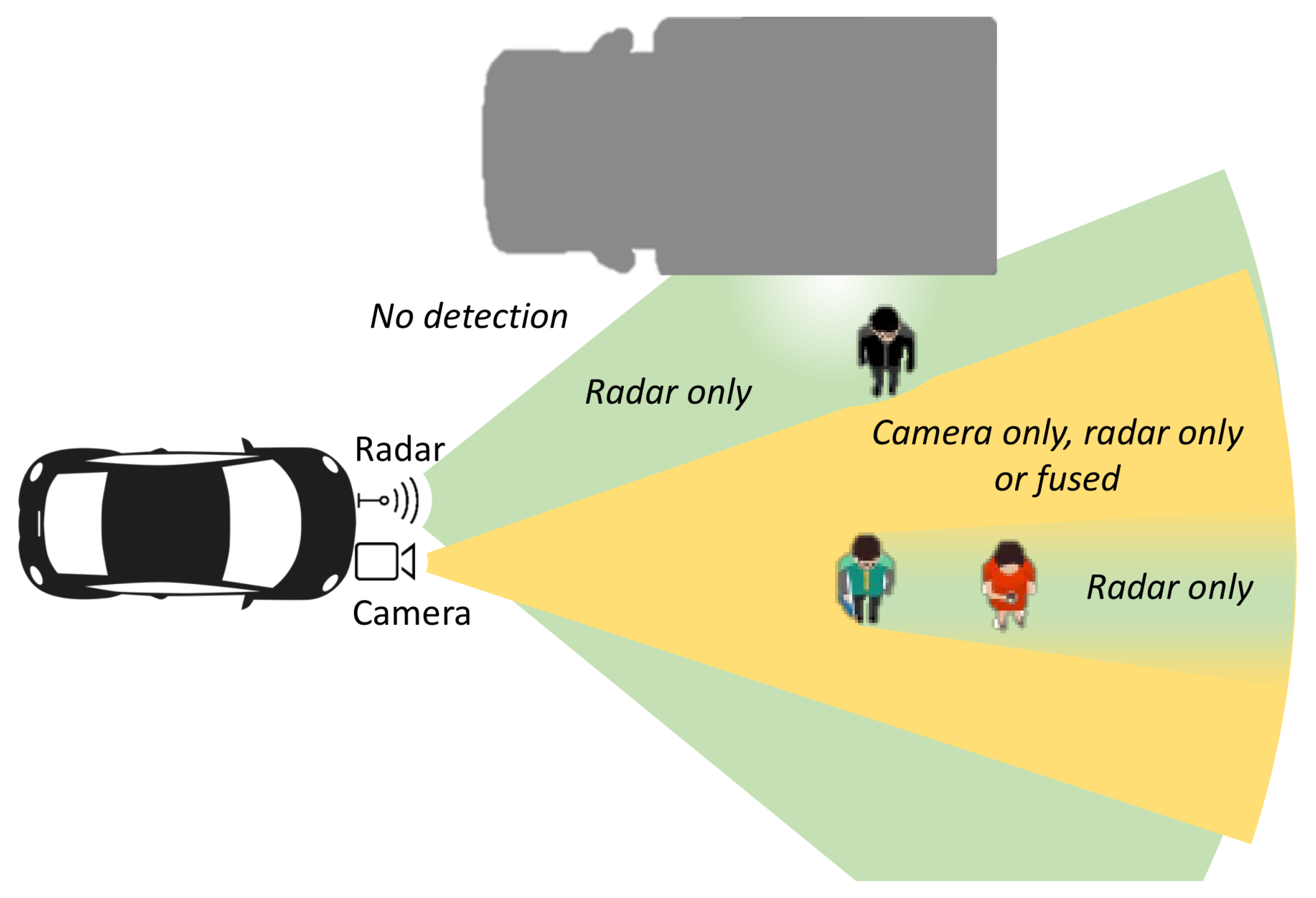
Figure 3 presents one typical sensor layout designed for environmental perception in front of a vehicle. Due to the different sensor fields of view (FoV), different regions of the environment are covered by none, one or both sensors. Moreover, it can be expected that the characteristics of sensor operation change locally depending on the scene layout. For the camera, every occluding object creates blind spots where misdetection is likely. On the example layout on
Figure 3, the person in red cannot be detected by the camera because of occlusion. However, this occluded region in the camera, although attenuated, is still visible by radar. Using radio wave propagation principles we can expect that any occluding object within the first Fresnel zone, an ellipsoid with radius:
will degrade the signal strength.
is defined through
c, the speed of light in the medium, the distance
D between the transmitter and receiver, and
f the wave frequency. In practice, the first Fresnel zone should be at least
free of obstacles for a good signal. For a person standing at 20 m in front of the radar, the radius of the first Fresnel zone for a 77 GHz radar beam is roughly 20 cm. If a person is occluding this first Fresnel zone, it will not create a complete radar occlusion because gaps between the parts of the body allow for signal propagation. The radar signal will nevertheless be attenuated. Additional problems for radar detection come from the effect of multipath propagation caused by reflections from flat surfaces (walls, large vehicles, etc.). On the diagram on
Figure 3 this is visualized as a hole in the radar frustum near the flat surface of a truck. In such areas, the radar signal fades significantly and detection rates reduce accordingly. Very near to flat surfaces, the radar mode of operation can even switch to a degenerate one even though the area is well within the radar FoV. Incorporating such prior information about sensor coverage zones requires accurate knowledge of the 3D scene. This knowledge is difficult to compute in real-time systems as it depends upon ray-tracing of camera as well as radar signals in the scene. Instead of precisely modeling the frustums of each sensor, we let the SOMPF tracker determine the sensor operating mode from the characteristics of the associated detections over time. To that end we propose an intermediate-level fusion technique for integrating radar and camera information prior to applying detection threshold, which results in a set of fused measurements
as if they were produced from a single sensor with multiple, locally varying, observation models. This fused sensor covers the area of the union of original sensors. Thus, the problems which arise in modeling intersections and unions of sensor frustums are handled elegantly in a single model.
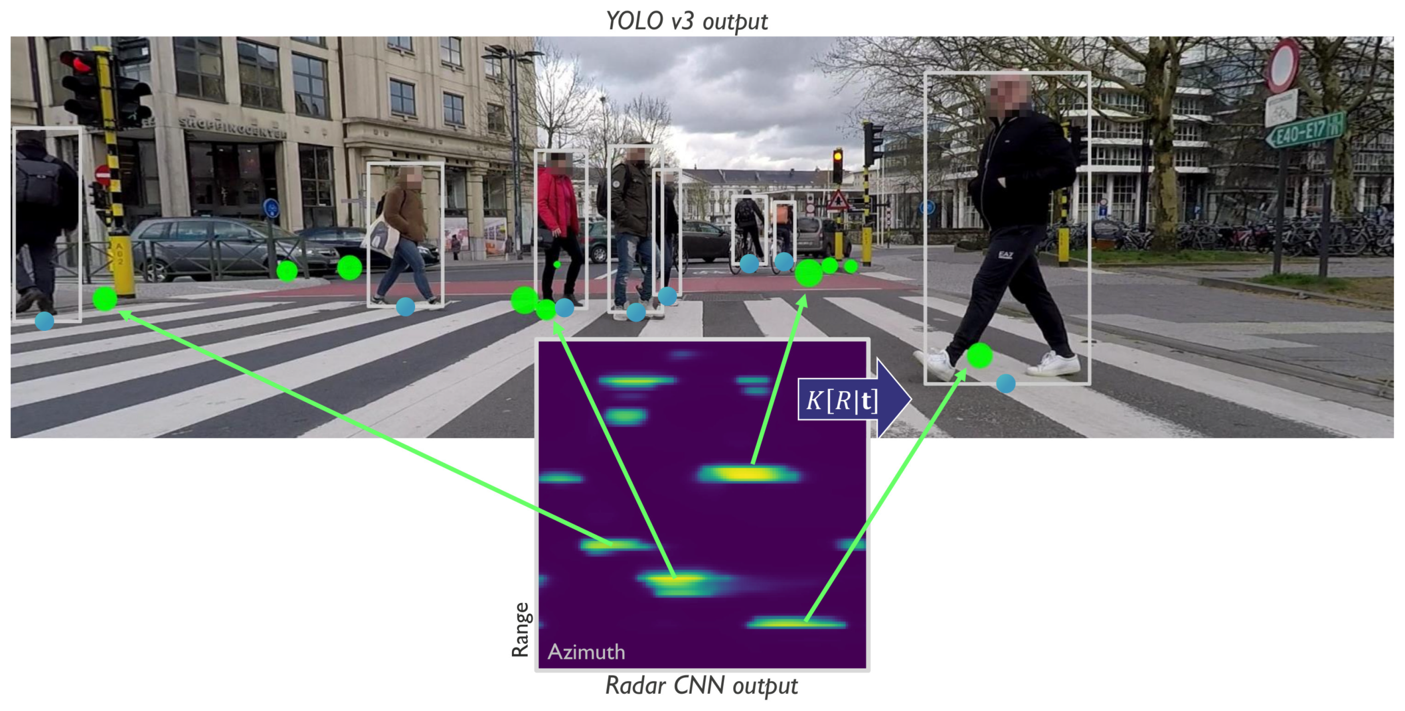
Detection starts by running independent object detection CNNs on the raw image and radar data. The employed camera detector, YOLOv3 [
8], outputs a set of bounding boxes, while the radar detection CNN [
7] outputs an array of VRU detection scores in polar coordinates, visualized on
Figure 1. We interface with both detectors prior to applying a detection threshold and obtain a complete set of detection candidates. These candidate detections can be considered as intermediate-level outputs as they exert a high recall rate, but also contain many false positives. Due to their high recall rate, objects detected confidently by one sensor, but not so well in the other can be used to reinforce one another’s detection scores. This concept of sensor-to-sensor cooperation can help improve detection rates in areas of poor visibility for one sensor and will be explained in more detail in
Section 4.2. After applying the sensor to sensor cooperative logic, we fuse the camera and radar mid-level detections by projecting and matching on the image plane. Detection fusion yields fused detections
which are matched based on proximity on the image, while their respective feature vectors
are formed using the feature vectors of the closest camera and radar target. We note that due to calibration and detection uncertainty, a fused detection can often contain only camera
or radar
evidence depending on how well the two sensors agree.
Compared to early fusion, our intermediate fusion algorithm reduces the data transfer rate, but retains most of the information useful for object tracking. Both object detection CNNs are built on the same hierarchical principle, that is, they first produce mid-level information consisting of object candidates (proposals) which are then further classified into VRUs. We detect radar detection candidates
within small neighborhoods
by means of non-maximum suppression of the radar CNN output, formally where every local maxima
is a vector consisting of the range and azimuth
of the detection peak and has a confidence score
equal to the peak’s height. The radar detections are distributed according the following observation model:
where
is the VRU position on the ground plane expressed in polar coordinates,
and
is a zero-mean bi-variate Gaussian distribution with a covariance matrix
of known values
. Using the extrinsic and intrinsic calibration matrices
we project each radar detection on the image plane where a detection maps to pixel coordinates
. Naturally, the uncertainty in azimuth projects to horizontal uncertainty on the image plane, thus radar detections have a much higher positional uncertainty in the horizontal direction than in the vertical. This uncertainty can be computed by propagating the ground plane covariance matrix
to image coordinates and estimating the image covariance matrix
of the newly formed random variables
. Due to the non-linearity of this transform, an interval propagation can be performed in order to compute intervals that contain consistent values for the variables using the first-order Taylor series expansion. The propagation of error in the transformed (non-linear) space can be computed using the partial derivatives of the transformation function. However, we found out that the parameters of the covariance matrix of radar projections on the image plane,
, can accurately be approximated by the following transformation:
where
and
are the horizontal and vertical camera focal lengths and
is the range of the radar target. Thus, for radar targets
on the image plane we can use the following observation model:
where
is the vector of image plane coordinates of the feet of a person at time
t and
is the radar covariance matrix in image coordinates
.
Similarly, we interface with the image detection CNN at an early stage where we gain access to all detections regardless of their detection score. Each camera detection consists of the image coordinates of the bounding box center as well as the BB width, height, appearance vector and a detection score:
. For modeling the image plane coordinates of the feet of a person detected by a camera detector,
, we use the following model:
where the covariance matrix
can be estimated offline from labeled data.
In order to match camera detections to radar detections on the image plane, we rely on the Bhattacharyya distance as a measure of the similarity of two probability distributions. Practically, we compute the Bhattacharyya coefficient of each camera and radar detection pair, which is a measure of the amount of overlap between two statistical samples. Using the covariance matrices
and
of the two sensors, the distance of any two observations
is computed as:
where
is the Bhattacharyya distance:
and the covariance matrix
is computed as the mean of the individual covariance matrices:
Closely matched detections form a fused detection
whose image features
(BB size and appearance) are inherited from the camera detection. For computing the ground plane position
, we need to project both camera and radar detections to the ground plane. Due to the loss of depth in the camera image, a camera detection
has ambiguous ground plane position. We can, however, use an estimate based on prior knowledge. Specifically, we make the assumption that the world is locally flat and the bottom of the bounding box intersects the ground plane. Then, using the intrinsic camera matrix we back-project this intersection from image to ground plane coordinates. This procedure achieves satisfactory results when the world is locally flat and the orientation of the camera to the world is known. In a more general case, back-projection will result in significant range error which we model with the following observation model:
where the the covariance matrix
consists of a radial standard deviation part
, a function of the distance:
and an azimuth standard deviation parameter
. Having both the radar and camera detection positions on the ground plane, we combine them using the fusion sensor model explained by Willner et al. and Durrant-Whyte et al. [
45,
46]:
where the covariance matrix
is computed as:
In practice, depending on how closely matched the two constituent detections are, a fused detection will obtain the range information mostly from the radar and the azimuth information mostly from the camera. On the other hand. the further apart the two constituent detections are, the more the fused target will behave like a camera-only or a radar-only target. In the special case when a camera detection is not matched to a radar detection
, the resulting fused detection will consists of only the assumed camera range and azimuth and the camera detection features
. Similarly, an unmatched radar detection yields a fused detection consisting of the radar range and azimuth, radar detection score and an assumed image plane BB
. In these cases, a fused detection is explained purely by the individual sensor model of either the camera Equation (
8) or the radar Equation (
2). Following the fusion method explained in [
45] the detection score is averaged from the camera and radar detection scores:
A potential weakness of averaging the detection scores of individual sensors becomes obvious when the operating characteristics of one sensor become less than ideal. We therefore propose a smart detection confidence fusion algorithm with the key idea of using the strengths of one sensor to reduce the other one’s weakness. The proposed algorithm produces significantly better detection scores in regions of the image with poor visibility caused by either low light, glare or imperfections and deformations on the camera lens. This is because radar can effectively detect any moving object regardless of the light level and its detection score be used to reinforce the weak image detection score. For closely matched pairs of detections where one sensor’s detection score is below a threshold, we will increase the detection score proportionally to the proximity and confidence of the other sensor’s detection. The resulting candidate object list recalls a larger amount of true positives at comparable false alarm rate.
Specifically, objects with a low detection score
, which are also detected by Radar
, will have an increased detection confidence proportional to the similarity coefficient in Equation (
6), formally:
where the parameter
controls the magnitude of reinforcement. Finally, after fusion and boosting, confident detections
are fed to the tracker where they are associated to a track
by optimizing the global detection to track association solution based on the association likelihood
.
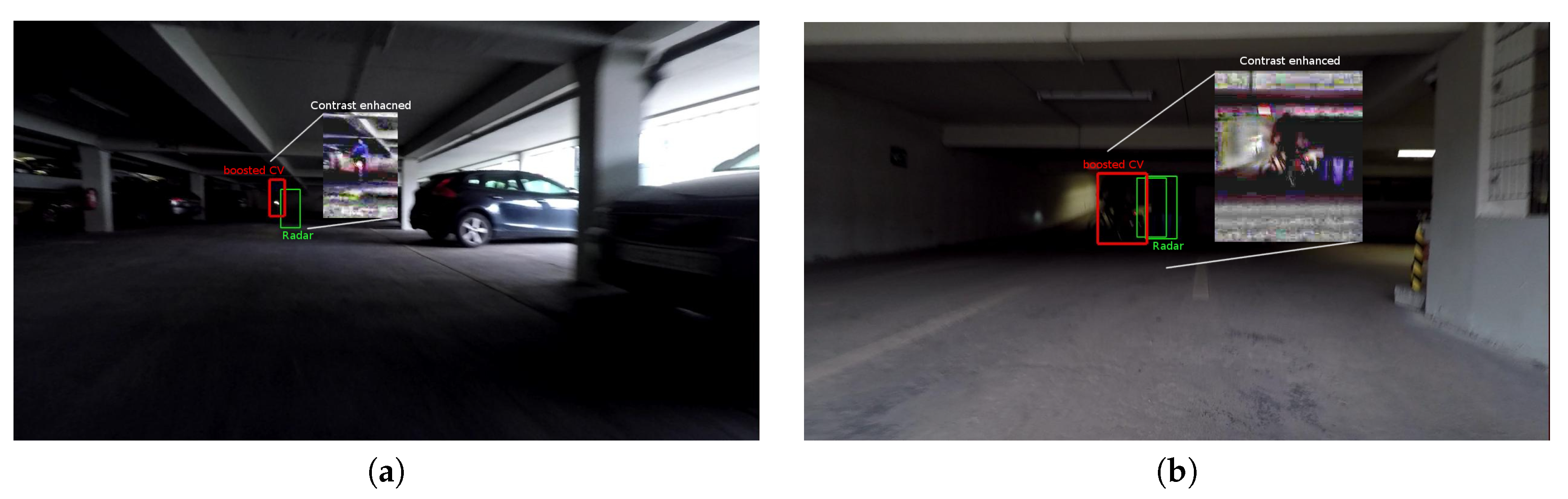
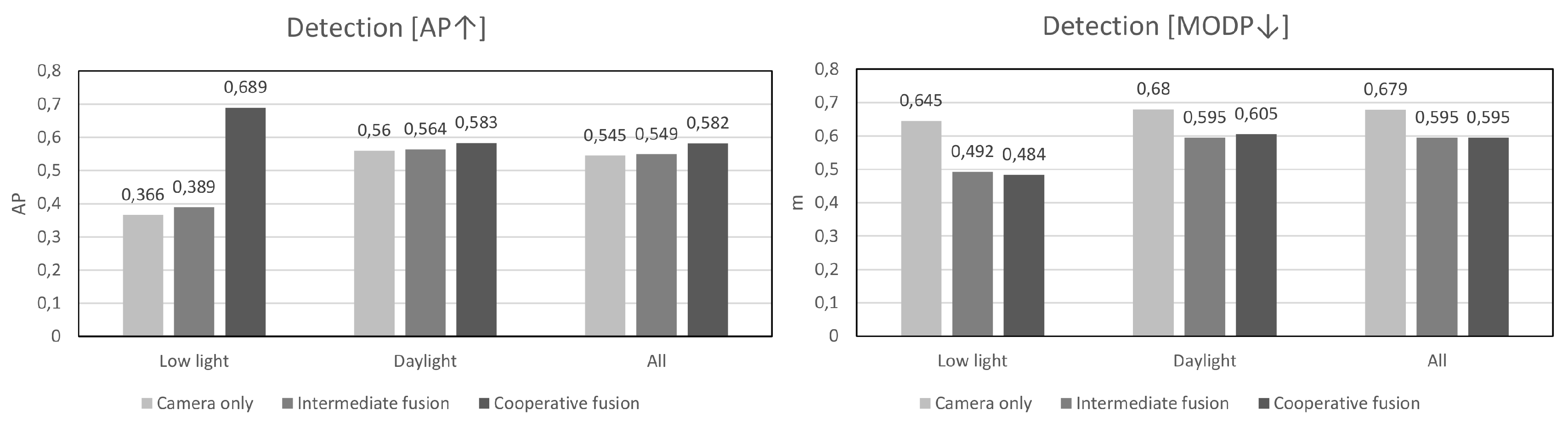
On
Figure 4 we present typical examples where the proposed cooperative fusion method brings significant improvements. In this poorly lit garage, people can be frequently seen exiting on foot from parked cars or on a bicycle from a bicycle parking area. Even in very low ambient light, the radar is able to accurately detect motion and thus boost low detection scores in suspected regions detected by the camera. Further numerical analysis of the performance is given in
Section 5 where we compare against a control algorithm that does not apply confidence-boosting.
4.3. Tracking by Detection Using Switching Observation Models
Assuming that at time
t the multiple detections
are optimally associated to tracks
by a detection-track association mechanism we will hereby explain the single target tracking algorithm which maximizes the belief of the state of a VRU by temporal integration of noisy measurements from multiple sensors. For the sake of notational simplicity we will drop the index “
” assuming that all detections underwent the data fusion steps in Algorithm 1. The state vector
consisting of the persons position and on the ground can be estimated from the probability density function (PDF)
by aggregating detections
over time. Due to the real-time nature of autonomous vehicle perception, we assume the Markov property whenever possible and confine to using recursive, single time-step operations. The process is governed by a state evolution model:
consisting of the nonlinear function
f and noise term
with known probability density
. The true nature of
f which explains the motion of a person on the ground plane, is dependent on both scene geometry as well as high-level reasoning which is difficult to model. Oftentimes in high frame-rate applications, human motion is commonly modeled using a constant velocity motion model which accurately explains human motion over such short time intervals. Each detection
, is related to a track
through the observation probability, or likelihood laws
discussed in Equations (
2), (
8) and (
9). The spatial component
models the likelihood that that an observation
stems from the state vector
on the ground plane, while the image component
models the likelihood of observing the image features
for the specific track
with features
, formally:
where
is usually inversely proportional to the Mahalanobis distance of the detection
to the sensor model centered around the posterior estimate
:
and
is a function measuring distance of image features such as BB overlap, shape or color similarity. In our previous work [
47] we have shown that an image plane likelihood consisting of the Jaccard index and the Kullback-Leibler divergence of HSV histograms between two image patches can be used as an excellent detection to track association metric, thus formally:
where
measures the intersection over union of the detection and track bounding boxes and while
is the Kullback-Leibler divergence of the detection and track HSV color histograms.
Depending on the external or internal conditions, our fused sensor can be operating in a specific state
c described by its specific observation function. We model the sensor state using the latent variable
c such that it can switch between categorical values explaining different sensing modalities. For example, detection of objects in good conditions can be considered to be a nominal state
and the detections can be explained through the nominal likelihood
in Equation (
14). In the further analysis we will drop the detection and track feature vectors,
and
, for the sake of notational simplicity. During operation, conditions can change dramatically due to changing light levels, transmission channel errors, battery power level. A camera will react to such changes by adjusting it’s integration time, aperture, sensitivity, white balance and so forth, which inadvertently results in detection characteristics different from the nominal ones. Any sensor, in general, can stop working altogether in cases of mechanical failure caused by vibrations, overheating, dust contamination and so forth. Additionally, manufacturing defects, end of life cycle, physical or cyber-attacks can alter the characteristics of measured data. Lastly, real-world sensor configurations employed to measure a wide area of interest often have “blind spots” where information is missing by design. All these factors can influence the current observation likelihood to be different from a nominal one.
For optimal tracking it is important to have a good model of the various modes of operation the sensor. Ideally, the chosen observation model should have the parameter flexibility to be able to adapt itself according to the gradual change of operation. Due to practical limitations in real-world operation, we are inclined to model only the most relevant sensor modes using discrete values for
c, for example a day-time and night-time camera characteristics or uncluttered and cluttered radar environment characteristics. We therefore use a list of observation models
where the appropriate sensor model
c is chosen at run-time through optimization. Thus, the sensor may switch between states of operation
. In a general case, for each sensor
there are
possible observation models, however since we are using detection fusion, our fused sensor can switch between the modes of operation of every constituent sensor:
where
is a nonlinear observation function and
is an observation noise of the observation model
at time
t. The following modes of operation are possible:
meaning that when a sensor is in a failure mode,
is statistically independent of
, the degenerate model
is used. In a nominal state of work
a sensor is assumed to be producing detections as it was indented by design, while in the other
j states of work the sensor is producing various levels of service. It is important to note that the sensor mode of operation also varies across the field of view. For camera and radar CNN object detectors this means that the detection quality will change in different regions of the field of view due to transient occlusions, light changes due to shadows or multi-path reflections which can cause an object detection score to briefly drop below the detection threshold. To complete the system we use a set of confidences that our fused sensor is in a certain state
which model the probability that the sensor is in a given operational state
:
Authors in [
43] state that these confidences are difficult to know a priori due to the possibility of rapid changes of external conditions and propose to tune them adaptively using a Markov evolution model. Thus the transition of probabilities
over time is:
with
being the vector consisting all individual
at time
t. The posterior PDF over the time interval
given the switching observation model formulation expands to:
where of practical interest is the marginal posterior at current time
, while the maximum a posteriori estimates
and
can be communicated to the chain of perception systems as the best estimates of a VRU position and the state of sensor at time
t. For estimation of the state vector
we rely on the estimation of the latent variable
for which, assuming they both have Markov property, Bayesian tracking can be employed. We adopt the same evolution model structure as proposed by [
43]:
where the Markov property of
results in a sensor state
dependent on its past values marginalized over
. The prior over the sensor state variables
being:
where the vector
needs to be estimated as well since it can vary over time and over the field of view of the sensors, for example, the reliability of a sensor decreasing over time. Because
models the confidence of the state of the sensor, and a sensor can only be in one state at a time, Equation (
19), we can effectively use the
-dimensional Dirichlet distribution
as a model for the evolution
. The intuition behind this distribution lies in the interpretation of the concentration vector
as a measure of how concentrated the probability of a sample will be. For example, if
the sample is very likely to fall in the
i-th component, that is, the sensor to be in that mode of operation. If
then the uncertainty of the sensor state will be dispersed among all components. For our fused sensor we propagate the confidences
from
as:
using the spread parameter
, that adjusts the spread of probabilities
, which is estimated using the evolution model:
where
is a zero-mean white Gaussian noise with known variance. The hyper-parameter transition function follows the density
and the authors in [
43] propose to use a Gaussian noise model with variances
that are also estimated. To reduce the complexity of the estimation process, in our approach we use fixed variances while the log function in Equation (
25) is used to ensure that the variances remain positive.
Finally, for the state evolution function
f in Equation (
13) we use a short-time behavioral motion model learned from annotated pedestrians walking in an urban environment. The current position and velocity is propagated from the past state using random changes in the longitudinal and lateral velocities, expressed in polar coordinates:
We refer the reader to find more details about this motion model in [
47].
4.4. Sampling-Based Bayesian Estimation
In applications such as VRU tracking in traffic scenarios, the posterior in Equation (
21) has a highly complex shape (often multi-modal) and cannot be computed in a closed form. For example, when a person becomes occluded for an extended time period, it is desirable to allow for multiple hypotheses to exist so that the same person can be accurately re-identified when detection evidence arrives. Additionally, camera and radar observation models are highly non-linear, making classical linear filters such as Kalman to become ineffective [
48]. To that end, we use the sequential Monte Carlo (SMC) method called particle filter (PF) which provides a numerical approximation of the state vector PDF using a set of weighted samples (particles). The tradeoff between estimation accuracy and computational load can be tuned by adjusting the number of particles in the filter. In a standard particle filter, each particle
with its corresponding weight
approximates the posterior PDF
through the empirical distribution
as:
where
is the delta–Dirac mass located in
. This distribution can be used to compute an estimate of the state vector, for example, the minimum mean squared error (MMSE) estimate is given as:
In practice however, it is more desirable to compute the maximum a posteriori (MAP) estimate of the PDF. It is easy to imagine a situation when the posterior PDF becomes strongly multi-modal, for example, when a person becomes occluded and can follow one of several possible paths of motion. The expected state PDF of such a person is then multi-modal with high probabilities for each model mean. A MMSE estimate will give a wrong result, so it becomes more useful to compute the MAP estimate
through one of the many mode finding techniques. For example, kernel density estimation (KDE) can be used to select the region of space with the highest probability:
where
K is a 2-D positive kernel function. In our switching observation model particle filter, estimation of the posterior in Equation (
21) from the system evolution models in Equation (
22) can be performed by applying the following steps:
Initialize the filter by drawing particles using their prior probability density functions: , , and set equal weights .
For each step perform sampling according to a proposal function q (or the transition model for bootstrap PF). For each particle sample the sensor state variable , the state vector , the probabilities and the hyper-parameter vector .
Update the weights using the new observation
using the appropriate observation model, with a slight abuse of notations:
and normalize the weights such that
.
Compute the effective sample size , approximately estimated from and re-sample when falls to some fraction of the actual samples (say ) in order to avoid the particle impoverishment problem.
The task of the proposal functions
q is to provide the most probable state space configuration at time
t given the newly observed data
. For the state vector
which explains the spatial object characteristics, the optimal proposal function
can be computed by applying the Kalman Filter update step for each particle
as explained by Van Der Merwe et al. [
49]. For the sensor state variable
Caron et al. [
43] approximate the optimal proposal
with an extended Kalman filter update step.Lastly, the proposal function for the probabilities
can be computed in closed form as given in [
43]:
where the individual components of the vector
are computed as:
for
This Switching Observation Model Particle Filter mechanism can be implemented relatively easily assuming that an observation
is available to guide particle sampling by proposal functions. However, in real-world multi-target tracking applications this is not always the case. As we previously discussed, multiple factors can cause detections to be missing which impacts the accuracy of the PF and sometimes even compromises its convergence. Therefore, it is of crucial importance to the trackers stability to accurately model missing observations.
4.5. Handling Missing Detections
Standard Monte-Carlo Bayesian filters perform sampling using a proposal function based on the new detection whereas weights are updated using Equation (
31). As detections become missing, sampling becomes compromised and weight updates are no longer possible. This is because the proposal functions are conditioned on the new detection. In this subsection we propose to use an adaptation of the multiple imputations particle filter (MIPF) for track updates when detections are missing. Originally introduced in the book by Rubin [
50] and later used in the papers [
39,
41], the MIPF extends the PF algorithm by incorporating a multiple imputation (MI) procedure for cases where measurements are not available so that the algorithm can include the corresponding uncertainty into the estimation process. The main statistical assumption in this approach is that the missing mechanism is missing at random (MAR). This means that the predisposition for a detection to be missing does not depend on the missing detection itself, but can be related to observed ones. For example, when a person being tracked becomes occluded by another person, one detection might not be correctly associated or even not reported at all by the detector. The missing detection is conditioned on the fact that there is a presence of an occluder, so, good techniques for imputing MAR data need to incorporate variables that are related to the missingness. We will show how in our application a detection
which is neither detected or associated to a track
can be approximated by sampling from a likelihood function without association at locations indicated by the prior, i.e., the estimated position
. This way our tracker can update the particles and track multiple hypotheses of a track until we have better evidence to decide which one is right. In the paper [
40], Zhang et al. provide more details about the MIPF and prove the almost sure convergence of this filter.
In our case of missing detections, we use the set
of indicator particles to explain this degenerate operation mode of the fused sensor. For the sake of notational simplicity we will drop the track and detection feature vectors
and
. We will use the auxiliary variable
to model missing observations which form the partitioned vector
This vector consists of
which corresponds to the missing part and
is the observed part of a detection’s ground plane coordinates. The switching observation model Particle Filter algorithm can then be applied irrespective whether
consists of
or
. Thus, depending on the origin of the peak
the observation model can switch between the following states:
Using the indicator variables, Equation (
18),
for the response of the sensor time
t, the posterior PDF, Equation (
21), can be written as:
where assuming that the missing mechanism is independent of the missing detections given the observed ones:
using the formulation in [
50] we rewrite the posterior as:
which means that the statistical model of the missing information is not necessary. In this special case, the posterior distribution as approximated in Equation (
28), can be computed using
amount of imputed particles:
where the multiple imputations
are not conditioned on past detections and the state transition equation. We adopt the proposed solution devised in [
40] to resolve this deficiency by drawing imputations from the missing data probability density which is unknown, but can be approximated from the posterior. Assuming no detections went missing prior to
t:
However, in order to get a good estimate of the posterior it is required that detections were present in the time instances leading up to the missing detection. Since we cannot sample directly from the updated posterior
(due to missing observation:
) we compute use an approximation by estimating posterior with no regard for missing data using Equation (
28). This means that the particles
are propagated using the state transition model to obtain an estimated PDF, formed by
and
. In practice, a missing detection will almost certainly be caused by a localized change of sensor mode
due to the loss of signal strength, occlusion, ambiguous association or noise. An imputed detection can therefore be simulated using the sensor model and the expected position of the tracked object. At the moment of missing detection, we can let the sensor mode evolution model Equation (
22) choose the most likely course of evolution of
. It is safe to assume that the missing detection PDF is the same as that of the observed data,
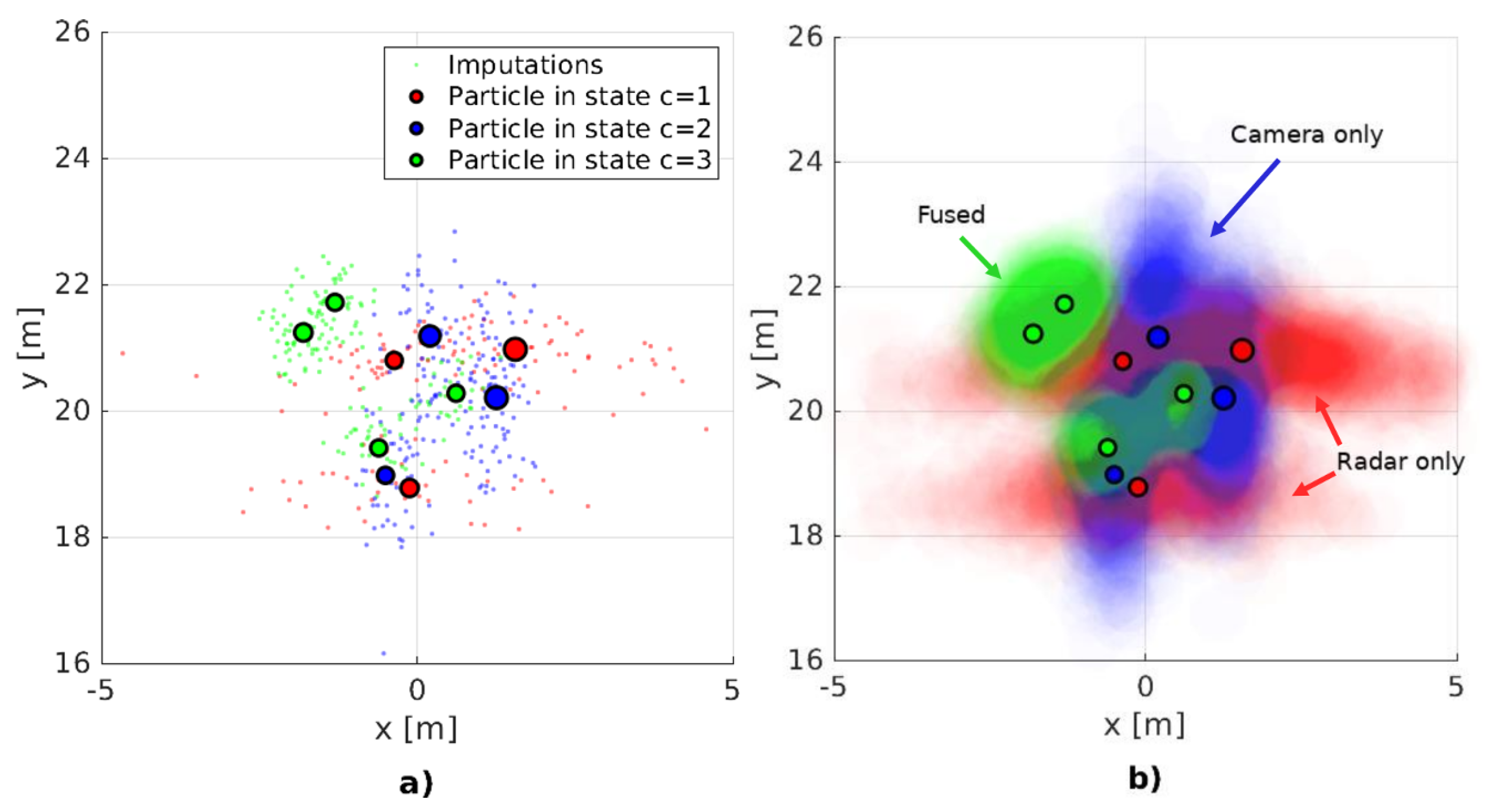
so we can use the imputation proposal function
from which we draw imputations
Practically, (
38) stipulates that the set of simulated detections (imputations) will be generated using the observation models defined by each particle
. This procedure is clearly illustrated on the two plots on
Figure 5. Thus, our definition of the fused sensor model, Equation (
33), for the missing detection case becomes:
According to Kong et al. [
51] we can use these complete data sets,
to compute an approximation of the posterior PDF. Substituting
in Equation (
36) yields:
where the approximate PDF is computed as the Monte Carlo simulation using
imputations. Thus, by substituting
into Equation (
37) we get:
which is computed by performing particle filtering treating each imputation
as a detection:
where
is the
i-th particle for the
j-th imputation at time
t and
is the respective weight estimated from the most likely observation model
. Finally, by substituting Equation (
43) into Equation (
42) we obtain a form to practically compute an approximation of the posterior PDF when observations are missing and replaced by imputations:
Two problems arise when applying the multiple imputations PF for real-time application. Firstly, its computation is prohibitively expensive because each time a detection is missing, the particle filter needs to perform
updates treating each imputation
as a simulated detection and then average the results; double sum in Equation (
44). The complexity lies mainly in the computation of the weights
which in most cases requires
evaluations of sensor model. Secondly, since we are dealing with a switching observation model, the accuracy of imputed particles relies on the accuracy of the estimates
which are in turn driven by available detections
from the past. In cases when detections are missing in short bursts, updating the evolution model Equation (
24) yields the most likely sensor mode
which can be accurate enough for drawing imputations and estimating the posterior PDF. However, when detections are missing over an extended time interval, for example, more than a few update cycles, the state transition models can quickly lead to an uninformative vector
, meaning that the states of all sensor mode particles
become equally likely. This results in diminished informativeness of the imputations and tracking becomes no better than using motion prediction alone. Thus, without accurate detection information, the tracker is very likely to diverge over time.
Our proposed solution improves the conditioning of imputations on the current sensor data which went missing for various reasons. Instead of sampling from the approximate proposal function in Equation (
40), for each position
of the posterior estimate
we compute the likelihood without to the closest detection without association
. Practically,
considers all possible detections
with no regard to detection thresholds:
where it is important to note that we do not use the
part of the image likelihood in Equation (
16). Using this method, the particle weight update can be performed as:
which is better conditioned on the sub-threshold sensor measurements compared to using no sensor measurements at all and thus relying only on the state evolution and sensor models in Equation (
39).
We argue that in the proposed detector-tracker design, the missing part
of a detection
often remains hidden bellow a detection threshold or it is discarded due to likelihood gating which safeguards against ambiguous associations. Therefore, by sampling from
it is possible to re-use the weak information in regions where a detection is indicated by the posterior
. In our proposed approach we draw a single
imputation
according to Equation (
45) and compute the weights
at locations
,
. Using this approach, simulated observations will be drawn from the posterior and their likelihood gets re-evaluated skipping the association algorithm. This approach has the practical implication that the computational load of updating the particle weights is reduced to a single computation per particle at the increased cost of finding for the closest detection in Equation (
45). However finding the closest detection
to each particle of any track
and thus the likelihood without association
can be performed efficiently by pre-computing this likelihood over a rasterized ground plane grid where each sector can be selected to cover a reasonably large area of equal likelihood. Thus, particles
falling within the same sector of
can share the same likelihood values without loss of information. Since we expect that in a real-world scenario there will be many missing detections, at each time step
t, we pre-compute the likelihood without association for each spatial location
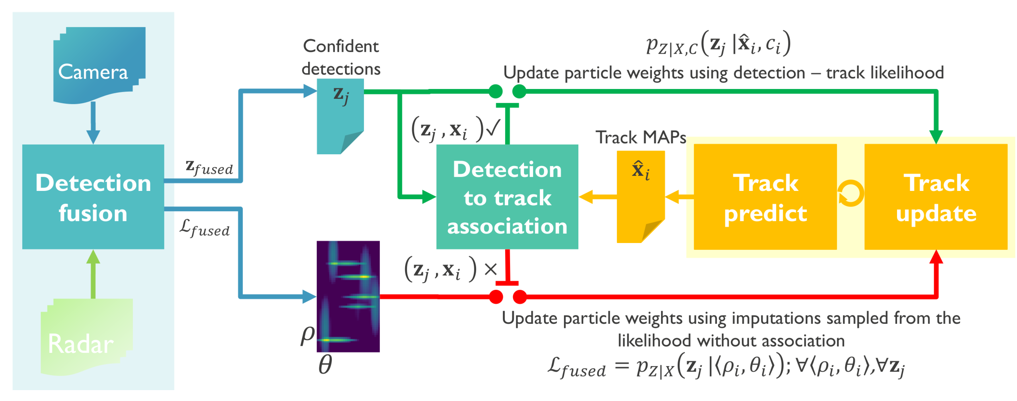
over a rasterized grid with range and azimuth density equal with that of the radar sensor. An example of one such grid is shown in the bottom part of the system diagram on
Figure 2. Whenever a track update needs to be made without a detection, the tracker can easily sample an imputation using this grid at
and use the values as a probability mass function. The downside to this approach is that we allow for the aggregated likelihood in
to update any unassociated track. This means that, in rare cases, multiple nearby and unassociated tracks can be updated using the same information which will inadvertently lead to tracks converging to each other and merging. However, one can argue that in such situations the limited evidence does not support the existence of more than one track and multiple hypotheses should be merged into one.
4.6. Bootstrap Particle Filter
Finding effective proposal functions
q is problematic since these functions have to approximate the unknown posterior distribution including all its modes as well as tails. When this posterior becomes multi-modal or heavy-tailed, the use of simple parametric proposal functions can lead to ill-informed sampling. In reality, this means that particles will be sampled near a single mode and/or not cover the tails of the actual distribution. It is known that the optimal proposal function, that is, the one minimizing the estimation error, is a multivariate Gaussian formed by applying a Kalman update step on each particle using the current observation. For each particle, a Kalman filter estimates the mean and covariance matrix of the multivariate Gaussian proposal distribution. The particle filter then draws new particles, each from their corresponding proposal distribution. Although this approach is proven to minimize the estimation error, details in [
43], it assumes the availability of observation
at each time step which is not guaranteed. The Kalman update step when data is missing is ill-posed, in a sense that imputations need to be drawn from a state estimate which needs a proposal function conditioned on the missing observation. Even in non-degenerate cases,
, running the (Kalman filter) KF update for each particle for multiple tracks is computationally prohibitive. Therefore, we choose to use the bootstrap particle filter [
46], which ignores the latest observation during the prediction step. Since the detection might be missing in the current step, the motivation for using the bootstrap PF is sound. The bootstrap PF uses the state and indicator variable evolution models as proposal functions making the particle weight updates in Equation (
31) depend only on the likelihood term:
This design choice makes increasingly more sense as the proportion of missing observations increases. Depending of the availability of the detection
, we either update the particle weights using the likelihood of the optimally associated detection Equation (
47);
or use the likelihood without association to draw imputations and update the particle weights with Equation (
46);
accordingly. In the latter case, the efficiency of the estimate can be approximated as
, expressed in units of standard errors, where
is the number of imputations and
is the fraction of missing information in the estimation, more details in [
50]. Finally, after the PF weights are updated the last step of the bootstrap particle filter is to apply importance re-sampling of the set of particles
to increase the effectiveness of the limited number of particles. Re-sampling can be performed at time intervals controlled by the effective sample size
as we explained in
Section 4.4.


