The PHY-layer simulator implements a complete LoRa transceiver (transmitter + receiver), thereby generating the modulated signal and performing the demodulation tasks, whereas the MAC layer simulator manages the channel multiple access, thereby implementing the data traffic (who transmits to whom and when), accounting for mutual interference and the presence of multiple gateways. Specifically, the simulator considers class A LoRaWAN devices (support of class C is also available) operating in the EU 863–870 MHz ISM band, and supports a number of features, including both uplink and downlink communications, imperfect SF orthogonality, capture effect, full/half-duplex GW operation, uplink-downlink interference, DC limitations and energy consumption estimation.
The simulation tool is extremely flexible, as it allows one to tune a large number of parameters, related to the PHY layer, the LoRaWAN protocol and the network itself. The outcomes are provided in terms of overall delivery rate, for both uplink and downlink, and energy consumption values for the individual devices and the network as whole.
4.1. Offline Configuration Operations
Prior to the simulation execution, a configuration step must be carried out offline, which consists of the definition of the scenario (e.g., the network layout) and of a number of parameters, which rule the network behavior. This step is discussed hereafter.
Network layout configuration. For each simulation, an area of interest is defined by the user (by default, a circular shape is assumed), in which N EDs and G GWs are deployed either manually (e.g., where they are actually located in a real deployment), or automatically, in fixed (e.g., on a grid) or in random positions.
Radio propagation configuration. An Okumura–Hata channel model [
25] is implemented as the default model in the simulator, even though other channel models can be defined by the user. The power received by a GW,
, is computed as a function of the transmit power,
, as
, where
is the transmitting antenna gain;
is the receiving antenna gain;
L represents the path loss in dB,
where
f is the frequency in MHz,
is the height of the GW in m,
d is the distance between the transmitter and the receiver in km and
is the antenna height correction factor, which varies according to the frequency and the size of the city,
with
denoting the height of the ED antenna in m. It should be highlighted that (
9) is valid for large urban areas and
MHz. Finally,
s represents random channel fluctuations due to shadowing, modeled as a Gaussian random variable, with zero mean and standard deviation
; that is,
. The user can choose the transmit power
,
and the height of the EDs/GWs.
Note that the discussed layout and propagation models can be defined by the user manually based, e.g., on empirical measurements. The respective functionality is supported by the simulator.
Radio resource management configuration. The policy adopted for the choice of the SF can be defined by the user, along with the DC configuration. As for the former, the user can dictate a specific SF for each ED or let the simulator make a decision based on the ADR. With reference to the DC, instead, the DC constraints can be disabled or enabled; in the latter case, these are automatically satisfied according to the regional limitation reported in [
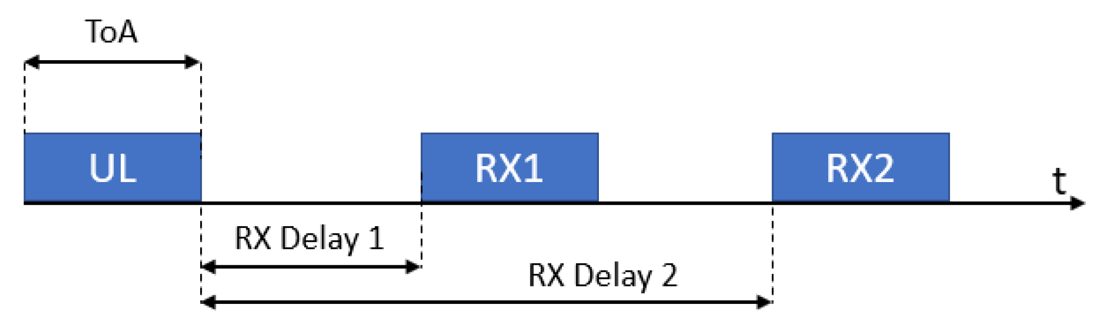
10]. In particular, DC limitations are specified according to LoRaWAN specification version 1.0.1, which dictates that a device (i.e., ED or GW), after sending a packet of duration ToA seconds, must not use the same frequency sub-band for the next
seconds. In addition, the user can also define the transmission parameters related to both RX windows. For RX1, the RX1DROffset parameter, which is the difference between the SF used in uplink and in RX1, is chosen by default according to
Table 4 (the user can introduce a different table, if needed). For RX2, instead, SF is fixed to 12 by the standard, even though the user can decide to change such parameter.
Data traffic configuration. The traffic generation models, for both the uplink and the downlink, are also configured by the user, along with the size of uplink and downlink packets in bytes ( and , respectively), the presence of the packet header H and the length of the preamble . When the default configuration is adopted, data packets are generated by EDs periodically every T seconds. The user can also define the probability of generating a downlink message after an uplink packet; by default, this is set to 1.
SIR threshold configuration. The MAC layer simulator is in charge of reproducing the ALOHA-based access protocol adopted by LoRaWAN, which does not depend on parameters to be configured. However, within the simulator this block also evaluates the signal-to-interference ratio (SIR) experienced by a receiver due to simultaneous transmissions, in order to check whether the packet is correctly received or not. As detailed in
Section 5, the SIR is compared with a threshold
, dubbed
SIR-threshold, which can be defined by the user. Clearly, evaluating the success/failure of a transmission in the presence of interference is by no means a MAC layer task; in the simulator perspective, however, the MAC layer simulator block is the most appropriate for the SIR assessment, because only this block knows which nodes (if any) are simultaneously transmitting hence might interfere each other.
Physical layer configuration. The bandwidth of the modulated signal is a user-defined parameter, along with the coding rate of the forward-error-correcting code adopted to reveal/correct transmission errors. Indeed, the encoding process should be carried out at the logical link control (LLC) sub-layer but, for the sake of simplicity, in our simulator it is carried out by the PHY-layer simulator. Note that in the current LoRaWAN specification both and are pre-specified for each region. Our models allow one to update these parameters, thereby adapting the simulator to other regions and/or novel modulation-coding schemes.
Table 5 summarizes the key parameters a user can define.
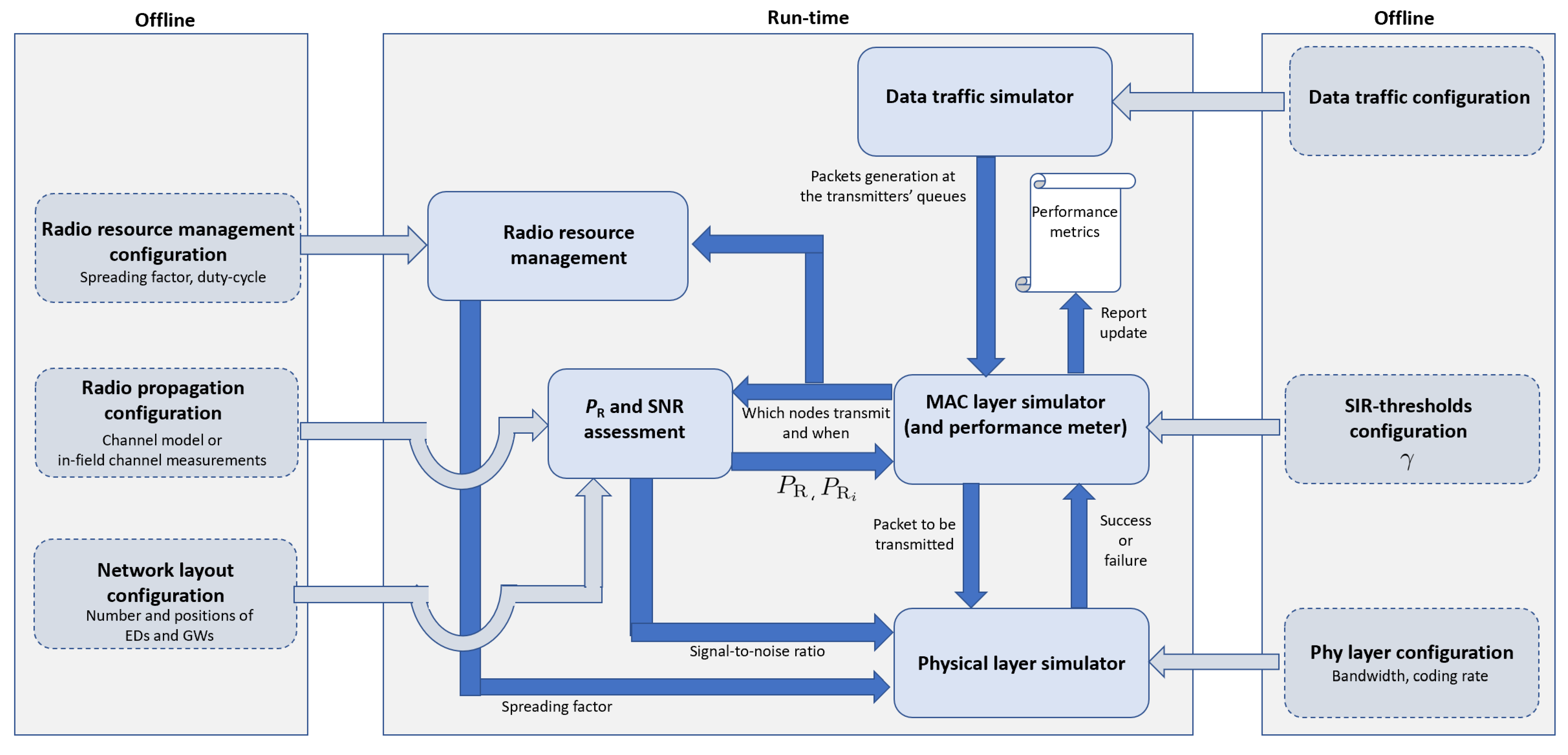
4.2. Run-Time Operations
During the execution, the data traffic simulator, which oversees the whole network, provides the MAC layer simulator with the time instants when data packets, generated either by EDs or GWs, enter the respective transmission queues. The MAC layer simulator, in turn, reproduces the behavior of the ALOHA channel access protocol for all devices in the network, thereby deciding which nodes, among those with queued packets, transmit and when.
This information is passed to the SNR assessment block that, given the positions of the transmitting nodes and the adopted channel model/channel measurements, derives the SNR experienced by receivers. Such information, along with the current SF value provided by the radio resource management, is used by the physical layer simulator, which generates the modulated signal corrupted by noise and demodulates it in order to assess if the packet is correctly received or not. Clearly, all accompanying operations, such as interleaving/de-interleaving, gray coding/decoding and channel coding/decoding, are carried out as well. The transmission outcome, either success or failure, is passed to the MAC layer simulator for any consequent action. The MAC layer simulator also gets from the SNR assessment block the values of the useful and interfering power at the receiver under investigation. This information is used to assess whether the interference level is such to prevent the correct reception. As detailed in
Section 5, this assessment is carried out by comparing the SIR experienced by the receiver under investigation and the SIR-threshold
. Given the result of such comparison and the success/failure outcomes of the physical layer simulator (which does not account for interference), the MAC layer simulator updates the performance counters, which are then used to compute the final performance metrics.


