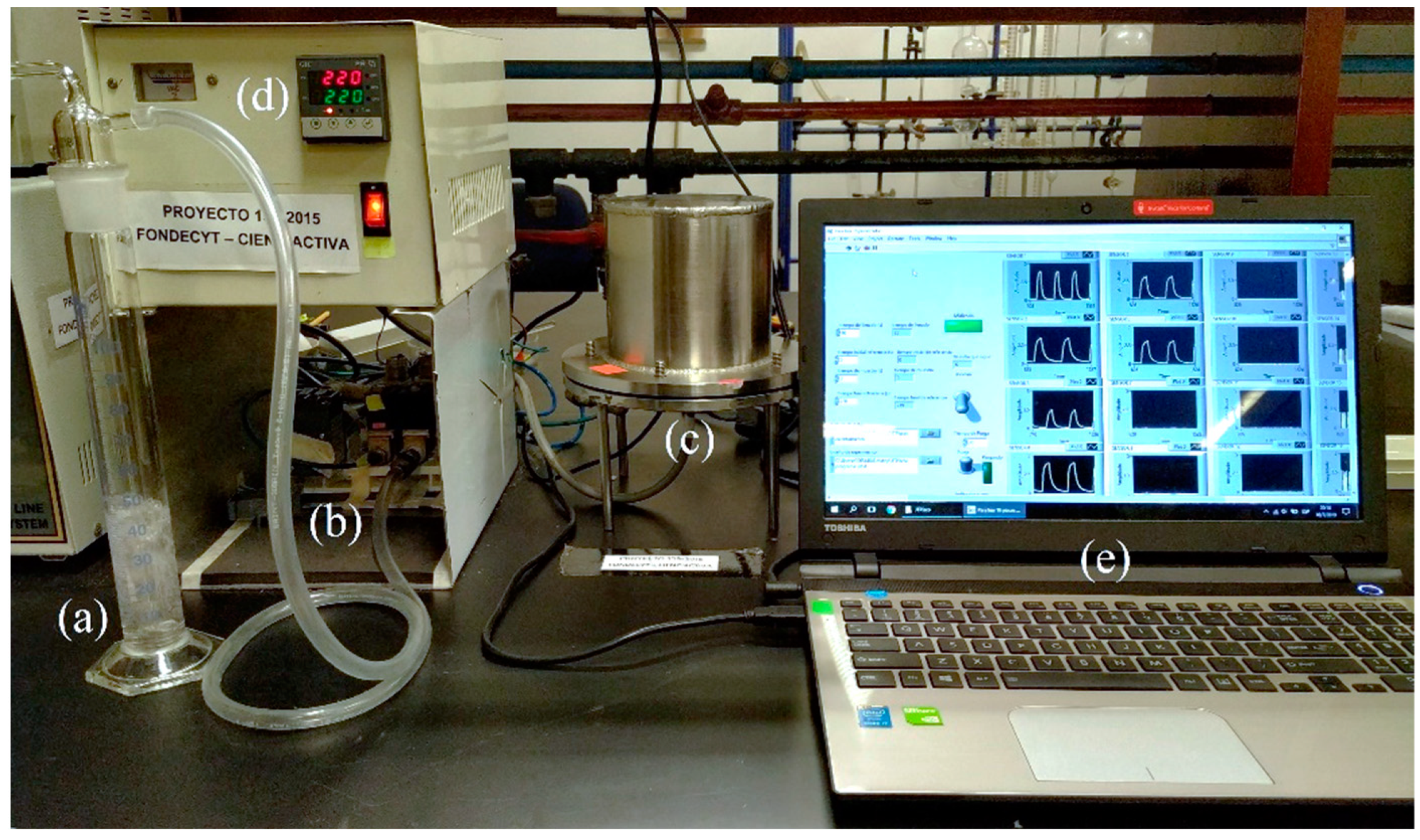
Figure 1.
Electronic nose. (a) Pisco sample, (b) hydraulic system, (c) sensing chamber, (d) temperature controller, (e) LabVIEW software interface.
Figure 1.
Electronic nose. (a) Pisco sample, (b) hydraulic system, (c) sensing chamber, (d) temperature controller, (e) LabVIEW software interface.
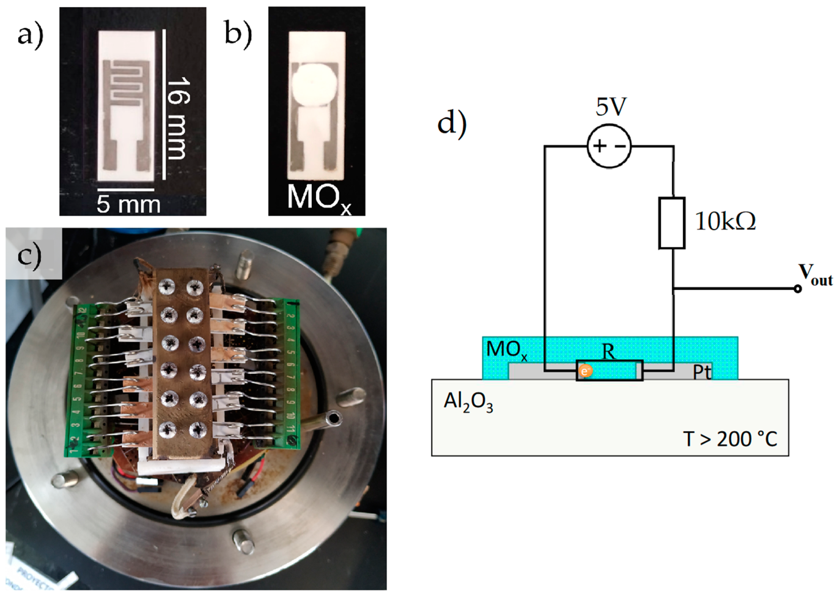
Figure 2.
(a) Platinum electrodes over alumina substrate, (b) gas sensor prepared from a metal oxide (MOx), (c) arrangement of sensors inside the sensing chamber, (d) schematic representation of the sensor.
Figure 2.
(a) Platinum electrodes over alumina substrate, (b) gas sensor prepared from a metal oxide (MOx), (c) arrangement of sensors inside the sensing chamber, (d) schematic representation of the sensor.
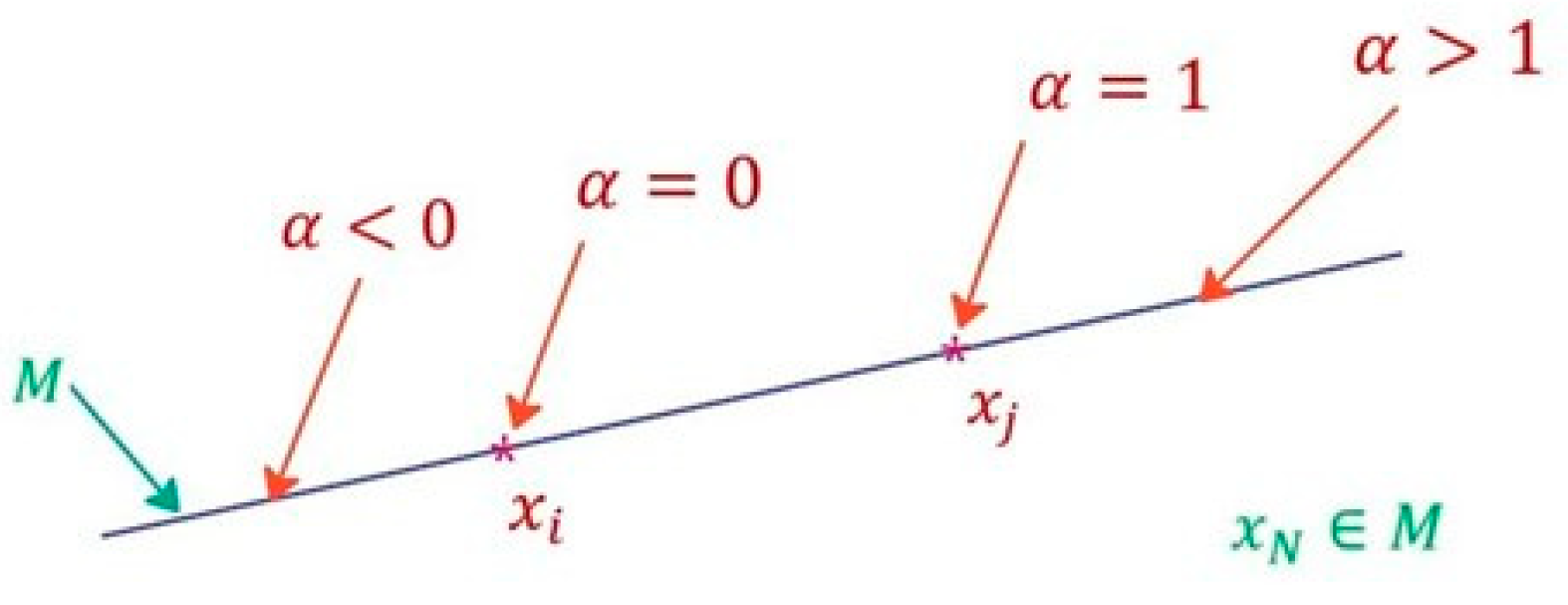
Figure 3.
Interpolation–extrapolation in the feature space for data augmentation. M is the set formed by the points of the blue line.
Figure 3.
Interpolation–extrapolation in the feature space for data augmentation. M is the set formed by the points of the blue line.
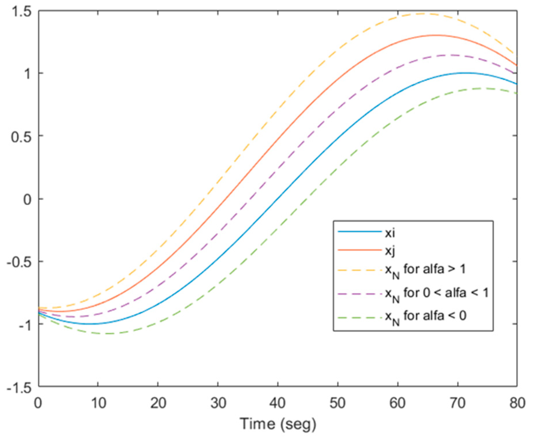
Figure 4.
Interpolation–extrapolation in the time domain for data augmentation.
Figure 4.
Interpolation–extrapolation in the time domain for data augmentation.
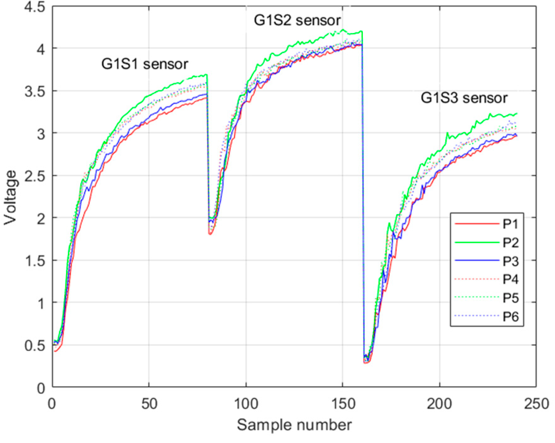
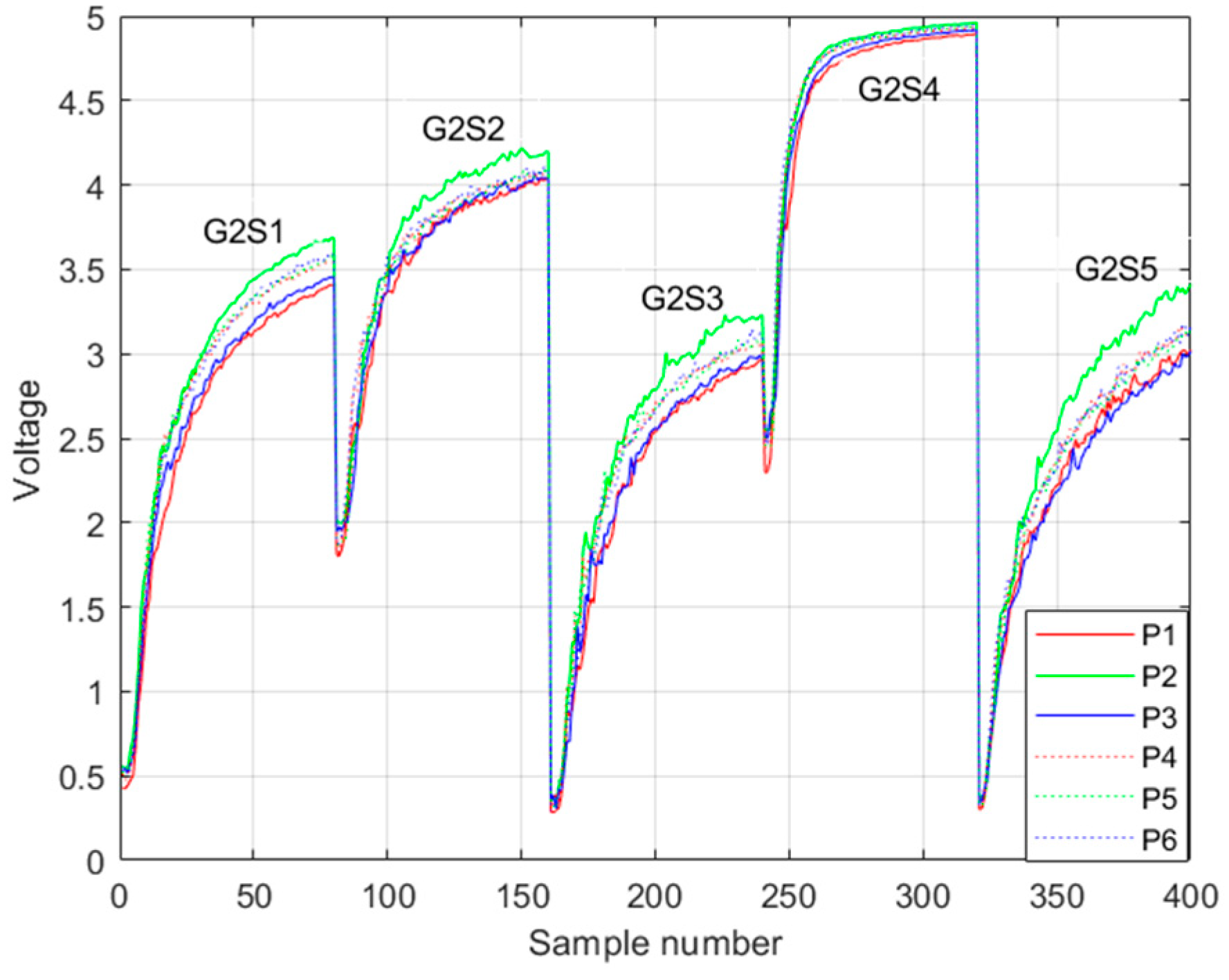
Figure 5.
Example of the rising voltage response of the first group of sensors in one trial. Legend Pi is the i-th class of pisco variety.
Figure 5.
Example of the rising voltage response of the first group of sensors in one trial. Legend Pi is the i-th class of pisco variety.
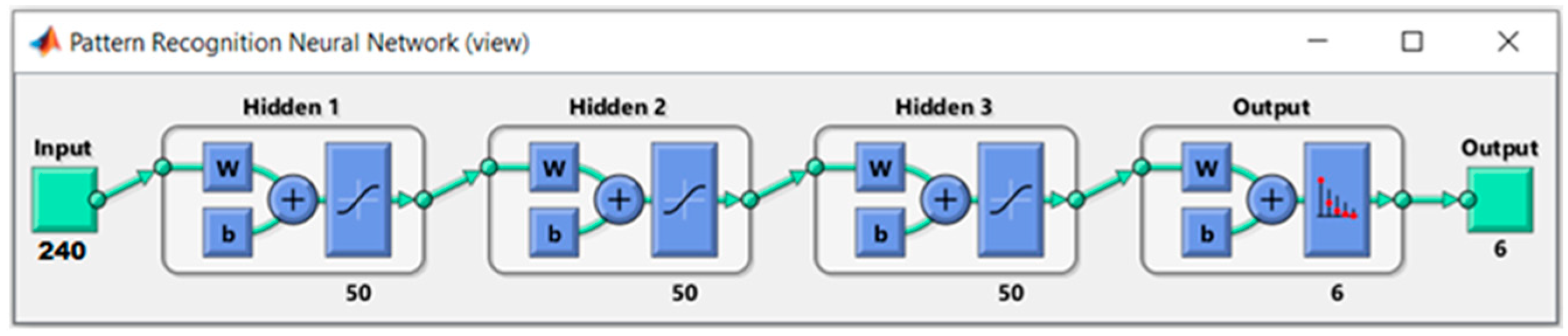
Figure 6.
Structure of the neural network to classify into 6 classes (varieties and brands).
Figure 6.
Structure of the neural network to classify into 6 classes (varieties and brands).
Figure 7.
Confusion matrix obtained after training the neural network without using augmented data.
Figure 7.
Confusion matrix obtained after training the neural network without using augmented data.
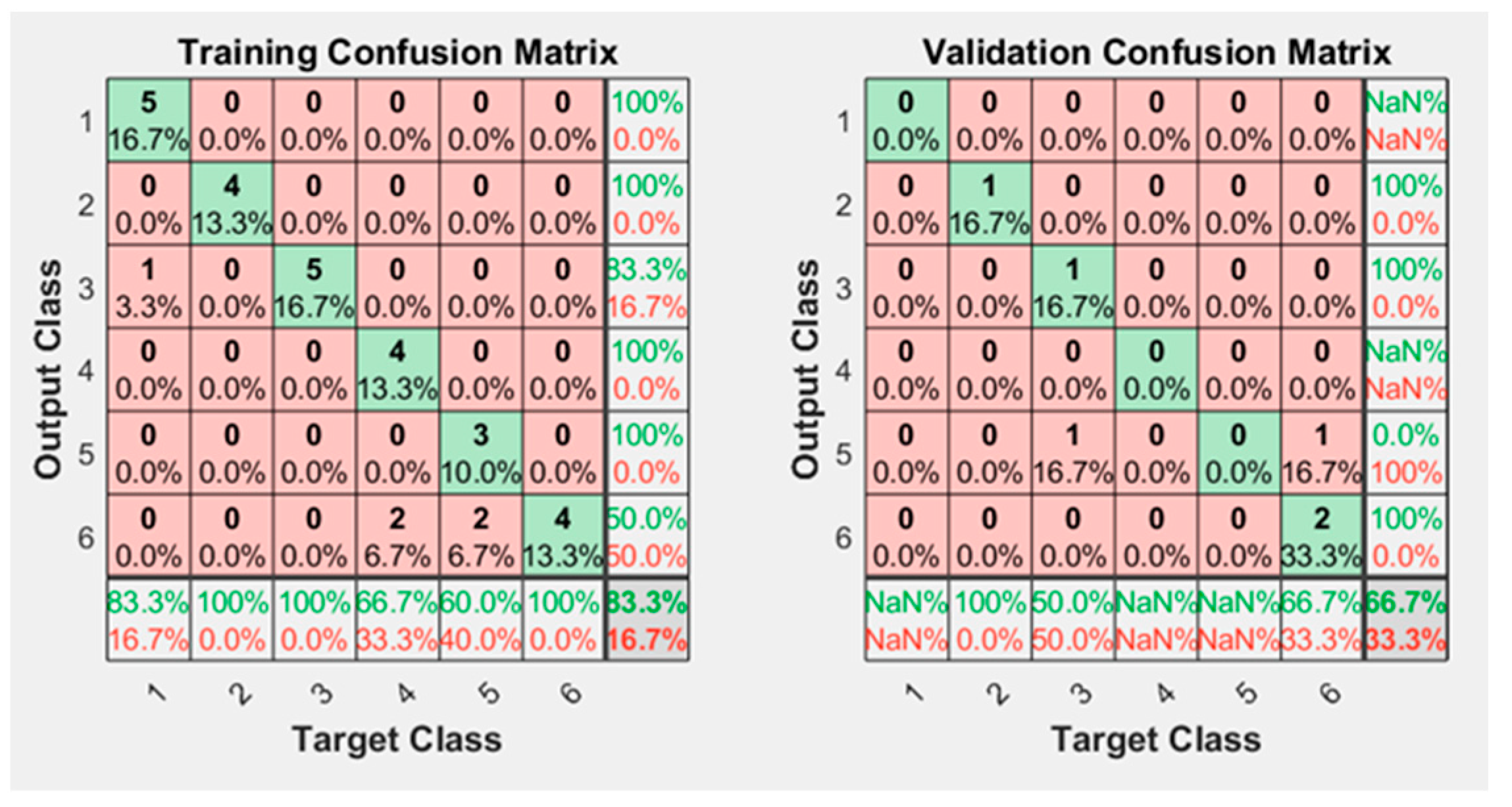
Figure 8.
Confusion matrix obtained after training the neural network using 2000 augmented data.
Figure 8.
Confusion matrix obtained after training the neural network using 2000 augmented data.
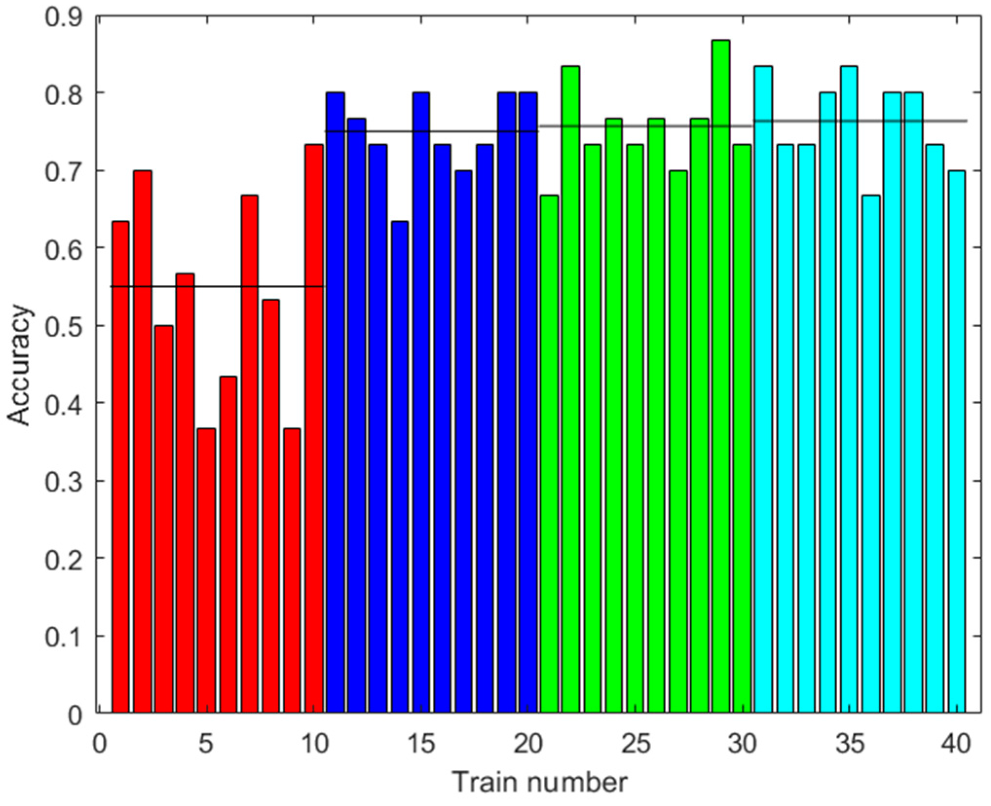
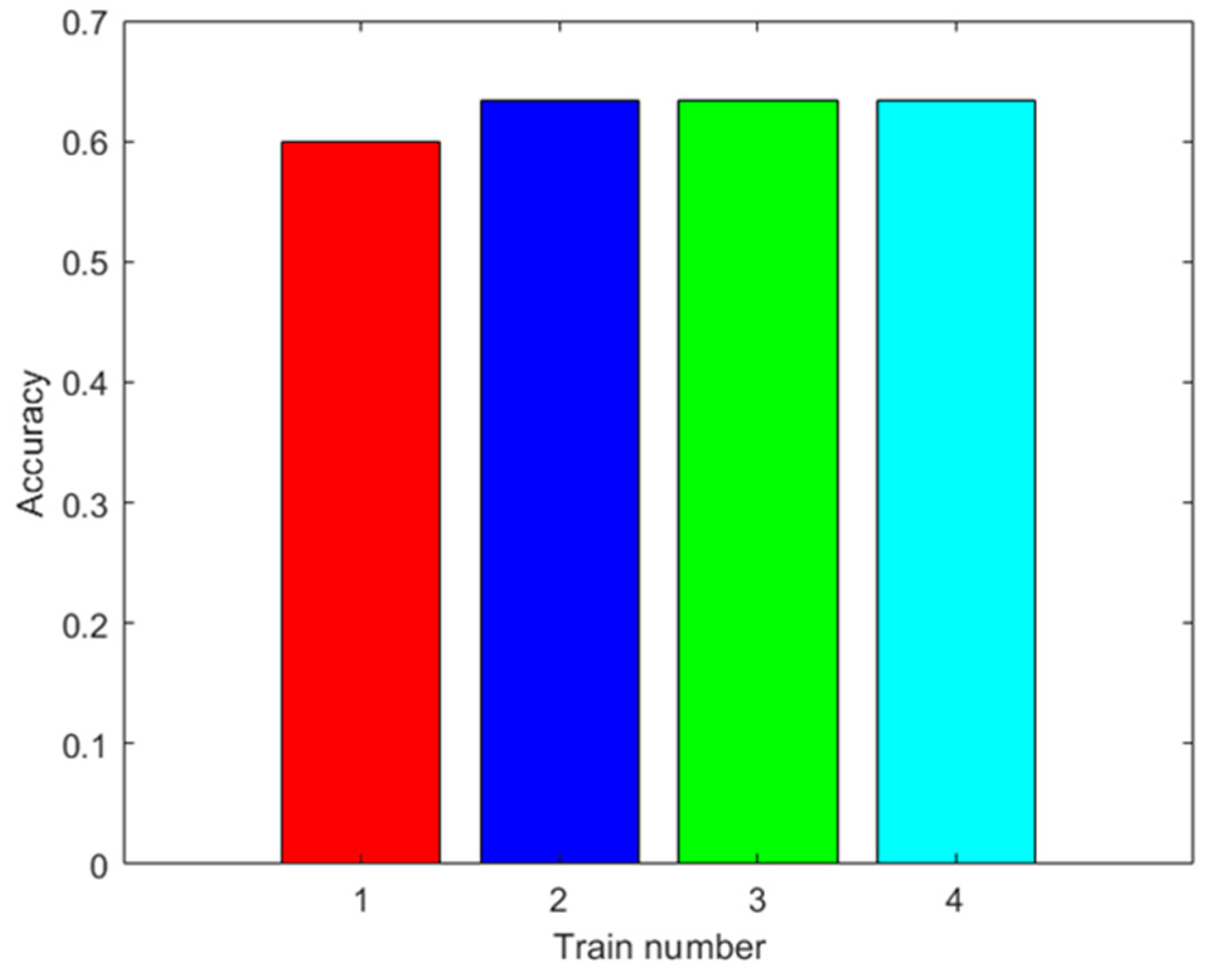
Figure 9.
Results with the first dataset. Accuracy of the prediction of the ANN with the test data after training with different amounts of augmented data (0: red; 100: blue; 500: green; 2000: light blue). Ten trainings were generated for each case. The black line shows the mean accuracy for each case.
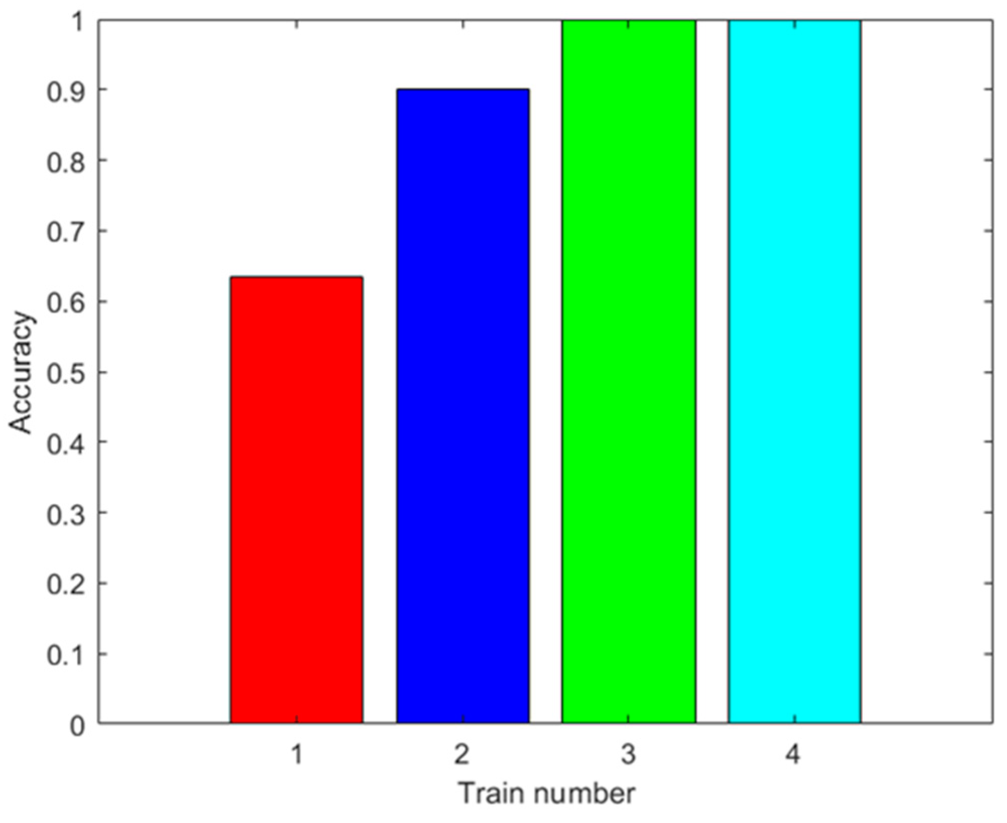
Figure 10.
Results with the first dataset. Accuracy of the MSVM prediction with the test data after training with different amounts of augmented data (0: red; 100: blue; 500: green; 2000: light blue).
Figure 10.
Results with the first dataset. Accuracy of the MSVM prediction with the test data after training with different amounts of augmented data (0: red; 100: blue; 500: green; 2000: light blue).
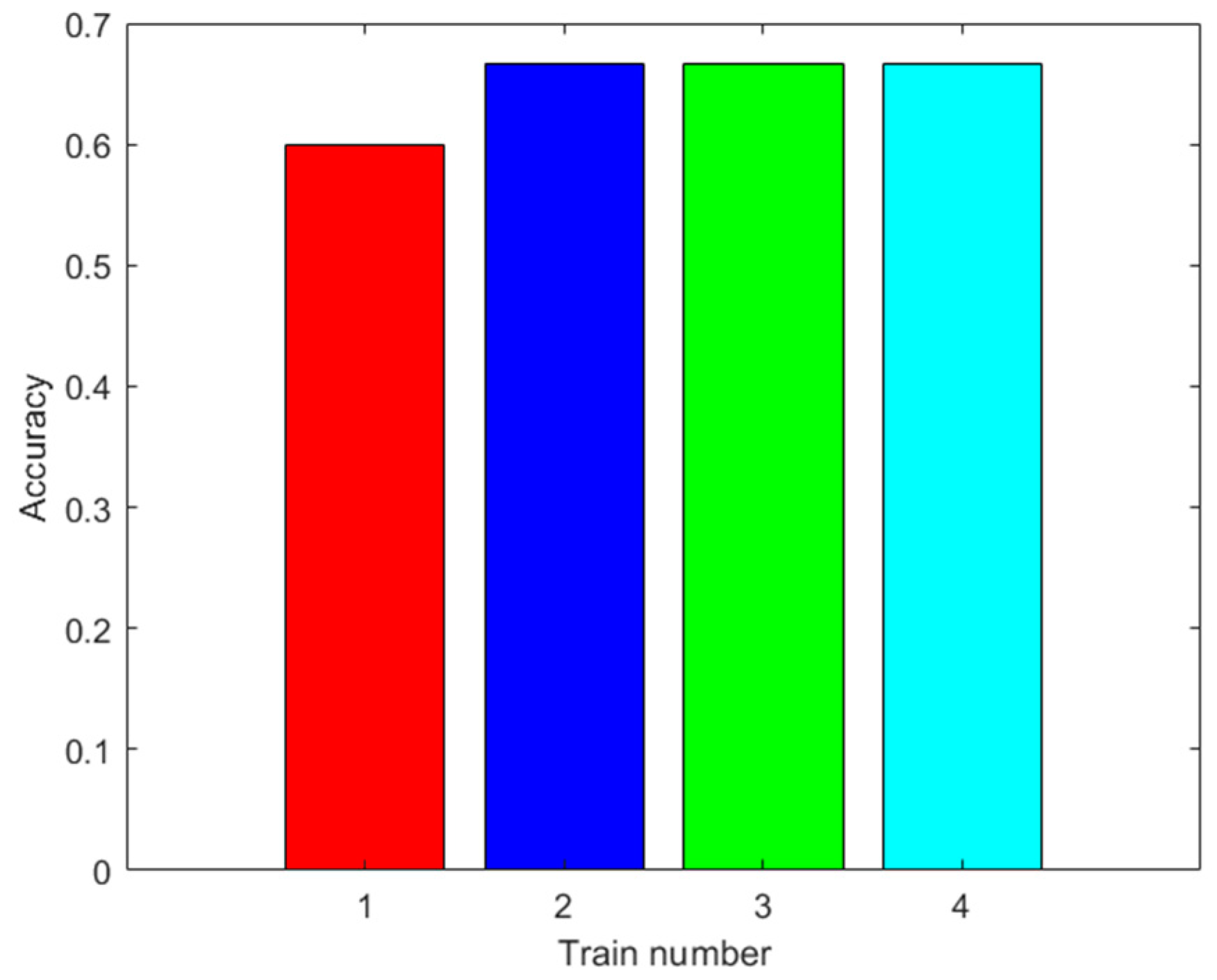
Figure 11.
Results with the first dataset. Accuracy of the RF prediction with the test data after training with different amounts of augmented data (0: red; 100: blue; 500: green; 2000: light blue). Ten trainings were generated for each case. The black line shows the mean accuracy for each case.
Figure 11.
Results with the first dataset. Accuracy of the RF prediction with the test data after training with different amounts of augmented data (0: red; 100: blue; 500: green; 2000: light blue). Ten trainings were generated for each case. The black line shows the mean accuracy for each case.
Figure 12.
Example of the rising voltage response of the first group of sensors in one trial. Legend Pi is the i-th class of pisco variety.
Figure 12.
Example of the rising voltage response of the first group of sensors in one trial. Legend Pi is the i-th class of pisco variety.
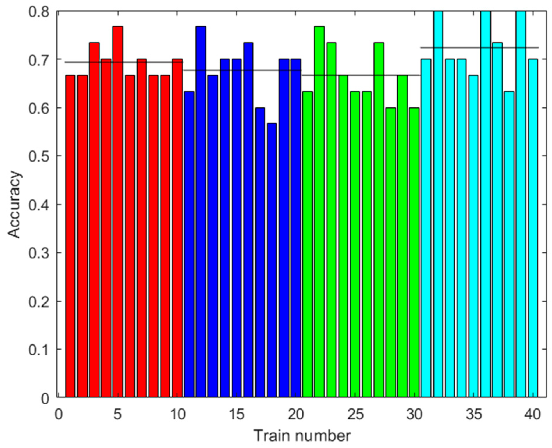
Figure 13.
Results with the second dataset. Accuracy of the ANN prediction with the test data. Training with different amounts of augmented data (0: red; 100: blue; 500: green; 2000: light blue). Ten trainings were generated for each case. The black line shows the mean accuracy.
Figure 13.
Results with the second dataset. Accuracy of the ANN prediction with the test data. Training with different amounts of augmented data (0: red; 100: blue; 500: green; 2000: light blue). Ten trainings were generated for each case. The black line shows the mean accuracy.
Figure 14.
Results with the second dataset. Accuracy of the MSVM prediction with the test data after training with different amounts of augmented data (0: red; 100: blue; 500: green; 2000: light blue).
Figure 14.
Results with the second dataset. Accuracy of the MSVM prediction with the test data after training with different amounts of augmented data (0: red; 100: blue; 500: green; 2000: light blue).
Figure 15.
Results with the second dataset. Accuracy of the RF prediction with the test data. Training with different amounts of augmented data (0: red; 100: blue; 500: green; 2000: light blue). Ten trainings were generated for each case. The black line shows the mean accuracy.
Figure 15.
Results with the second dataset. Accuracy of the RF prediction with the test data. Training with different amounts of augmented data (0: red; 100: blue; 500: green; 2000: light blue). Ten trainings were generated for each case. The black line shows the mean accuracy.
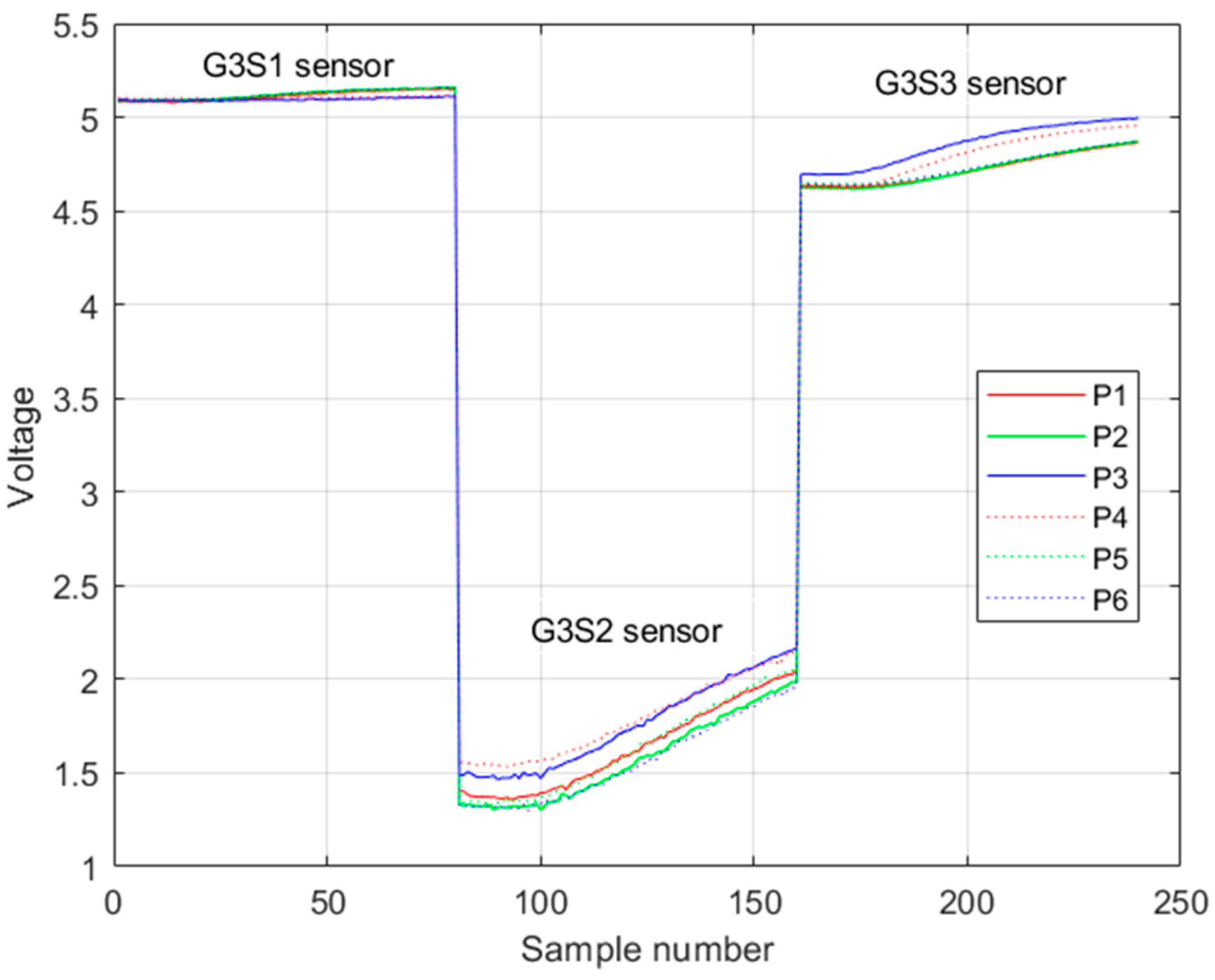
Figure 16.
Example of the rising voltage response of the third group of sensors in one trial. Legend Pi is the i-th class of pisco variety.
Figure 16.
Example of the rising voltage response of the third group of sensors in one trial. Legend Pi is the i-th class of pisco variety.
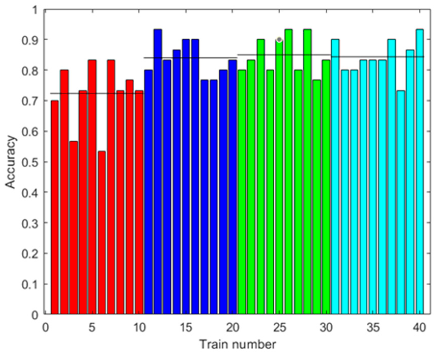
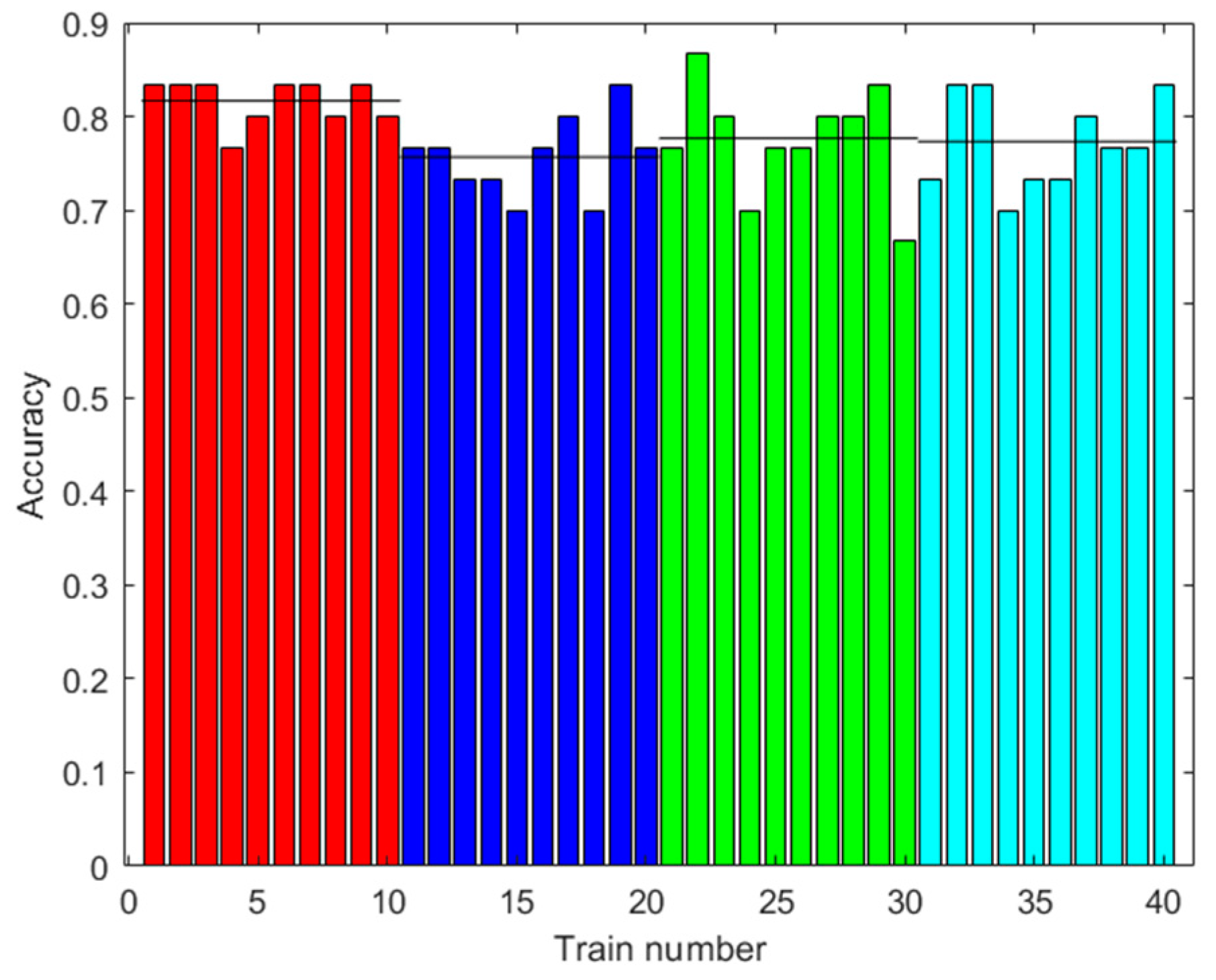
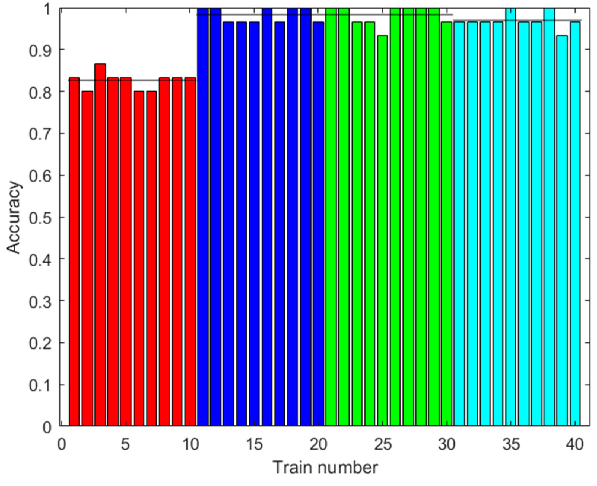
Figure 17.
Results with the third dataset. Accuracy of the ANN prediction with the test data. Training with different amounts of augmented data (0: red; 100: blue; 500: green; 2000: light blue). Ten trainings were generated for each case. The black line shows the mean accuracy.
Figure 17.
Results with the third dataset. Accuracy of the ANN prediction with the test data. Training with different amounts of augmented data (0: red; 100: blue; 500: green; 2000: light blue). Ten trainings were generated for each case. The black line shows the mean accuracy.
Figure 18.
Results with the third dataset. Accuracy of the MSVM prediction with the test data after training with different amounts of augmented data (0: red; 100: blue; 500: green; 2000: light blue).
Figure 18.
Results with the third dataset. Accuracy of the MSVM prediction with the test data after training with different amounts of augmented data (0: red; 100: blue; 500: green; 2000: light blue).
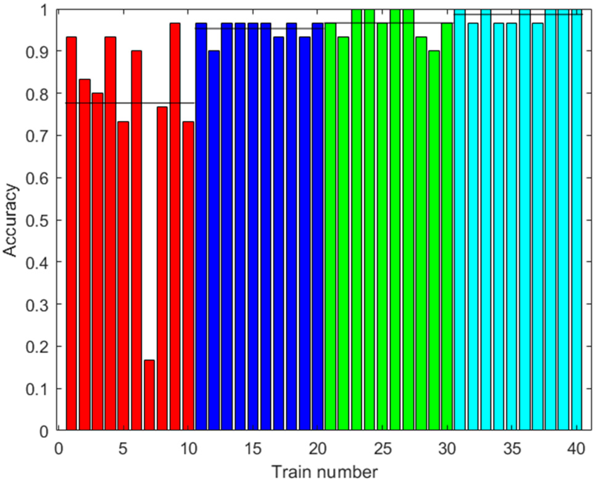
Figure 19.
Results with the third dataset. Accuracy of the RF prediction with the test data. Training with different amounts of augmented data (0: red; 100: blue; 500: green; 2000: light blue). Ten trainings were generated for each case. The black line shows the mean accuracy.
Figure 19.
Results with the third dataset. Accuracy of the RF prediction with the test data. Training with different amounts of augmented data (0: red; 100: blue; 500: green; 2000: light blue). Ten trainings were generated for each case. The black line shows the mean accuracy.
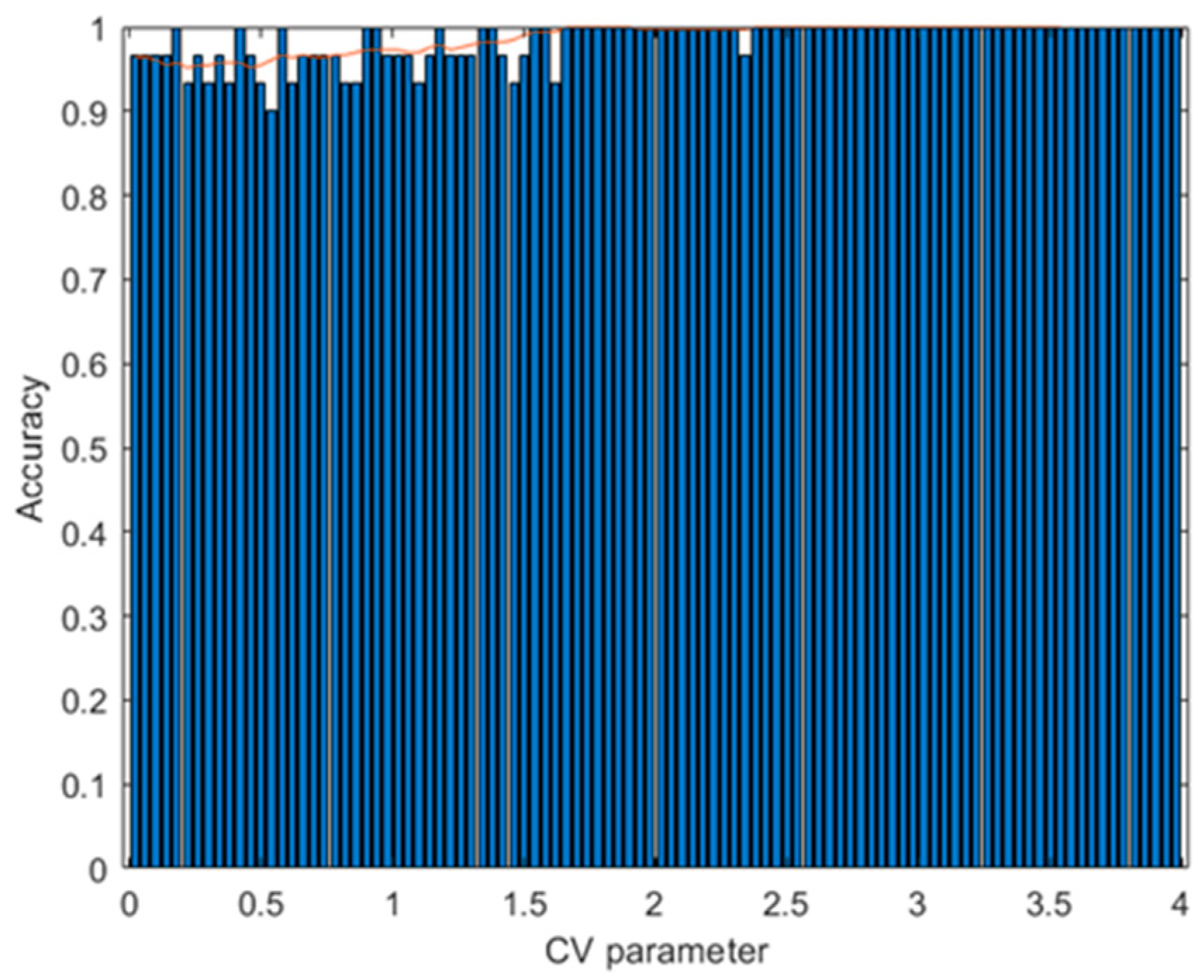
Figure 20.
Results with the third dataset. Accuracy of the ANN prediction with the test data as a function of the variation of the CV parameter. Training with 500 augmented data for each CV value. The red curve indicates the average of the bar and 10 subsequent values.
Figure 20.
Results with the third dataset. Accuracy of the ANN prediction with the test data as a function of the variation of the CV parameter. Training with 500 augmented data for each CV value. The red curve indicates the average of the bar and 10 subsequent values.
Table 1.
Peruvian pisco varieties analyzed.
Table 1.
Peruvian pisco varieties analyzed.
| Sample Number | Pisco Variety | Producer Abbreviation |
|---|
| 1 | Quebranta | T |
| 2 | Quebranta | D |
| 3 | Quebranta | Q |
| 4 | Italia | Q |
| 5 | Italia | T |
| 6 | Italia | D |
Table 2.
Sensors used in the electronic nose to obtain the first dataset.
Table 2.
Sensors used in the electronic nose to obtain the first dataset.
| Abbreviation | Composite Sensor |
|---|
| G1S1 | (SnO2/TiO2)-1:2-MK |
| G1S2 | (SnO2/MoO3)-1:1-MF |
| G1S3 | (SnO2/TiO2)-1:2-MF |
Table 3.
Sensors used in the electronic nose to obtain the second dataset.
Table 3.
Sensors used in the electronic nose to obtain the second dataset.
| Abbreviation | Composite Sensor |
|---|
| G2S1 | (SnO2/TiO2)-1:2-MK |
| G2S2 | (SnO2/MoO3)-1:1-MF |
| G2S3 | (SnO2/TiO2)-1:2-MF |
| G2S4 | (SnO2/TiO2)-1:1-MF |
| G2S5 | (SnO2/TiO2)-1:1-MK |
Table 4.
Sensors used in the electronic nose to obtain the third dataset.
Table 4.
Sensors used in the electronic nose to obtain the third dataset.
| Abbreviation | Composite Sensor |
|---|
| G3S1 | (SnO2/TiO2)-4:1 |
| G3S2 | (SnO2/TiO2)-1:4 |
| G3S3 | (SnO2/TiO2)-1:2 |
Table 5.
Results obtained with augmented data (AD) using the second dataset, the ANN machine learning algorithm and different data augmentation methods.
Table 5.
Results obtained with augmented data (AD) using the second dataset, the ANN machine learning algorithm and different data augmentation methods.
| Data Augmentation Method | Accuracy (%) |
|---|
| | 100 AD | 500 AD | 2000 AD |
|---|
| Proposed | 84.00 | 85.00 | 84.33 |
| Signal stretching | 84.67 | 86.67 | 85.00 |
| Gaussian noise and signal stretching | 80.67 | 82.00 | 84.00 |
| SMOTE | 74.67 | 77.00 | 78.00 |
| Gaussian noise | 76.33 | 73.67 | 70.67 |
Table 6.
Results obtained with augmented data (AD) using the second dataset, the ANN machine learning algorithm, different data augmentation methods and alternative test data.
Table 6.
Results obtained with augmented data (AD) using the second dataset, the ANN machine learning algorithm, different data augmentation methods and alternative test data.
| Data Augmentation Method | Accuracy (%) |
|---|
| | 100 AD | 500 AD | 2000 AD |
|---|
| Proposed | 92.67 | 93.00 | 91.33 |
| Signal stretching | 84.33 | 84.00 | 87.67 |
| Gaussian noise and signal stretching | 83.33 | 83.67 | 86.67 |
| SMOTE | 88.33 | 88.67 | 85.67 |
| Gaussian noise | 84.00 | 87.33 | 85.67 |
Table 7.
Results obtained with augmented data (AD) for different algorithms and datasets.
Table 7.
Results obtained with augmented data (AD) for different algorithms and datasets.
| | 1st Dataset—Accuracy (%) | 2nd Dataset—Accuracy (%) | 3rd Dataset—Accuracy (%) |
|---|
| | 0 AD | 100 AD | 500 AD | 2000 AD | 0 AD | 100 AD | 500 AD | 2000 AD | 0 AD | 100 AD | 500 AD | 2000 AD |
|---|
| ANN-1-5 | 57.33 | 66.00 | 67.67 | 67.67 | 51.33 | 79.33 | 80.00 | 81.00 | 78.33 | 92.67 | 96.67 | 97.33 |
| ANN-1-25 | 66.67 | 73.33 | 73.33 | 73.33 | 73.33 | 84.33 | 84.33 | 84.33 | 90.67 | 99.33 | 98.00 | 99.33 |
| ANN-3-50 | 55.00 | 75.00 | 75.67 | 76.33 | 72.33 | 84.00 | 85.00 | 84.33 | 77.67 | 95.33 | 96.67 | 98.67 |
| ANN-5-75 | 50.67 | 70.00 | 69.00 | 71.33 | 70.33 | 79.33 | 81.67 | 84.33 | 95.67 | 100.00 | 100.00 | 100.00 |
| MSVM | 60.00 | 63.33 | 63.33 | 63.33 | 60.00 | 66.67 | 66.67 | 66.67 | 63.33 | 90.00 | 100.00 | 100.00 |
| RF | 69.33 | 67.67 | 66.67 | 72.33 | 81.67 | 75.67 | 77.67 | 77.33 | 82.67 | 98.33 | 98.33 | 97.00 |
| PCA-2-MSVM | 56.67 | 43.33 | 46.67 | 50.00 | 43.33 | 40.00 | 50.00 | 46.67 | 56.67 | 73.33 | 80.00 | 80.00 |
| PCA-3-MSVM | 60.00 | 60.00 | 66.67 | 66.67 | 60.00 | 70.00 | 63.33 | 66.67 | 63.33 | 86.67 | 93.33 | 90.00 |
| PCA-6-MSVM | 60.00 | 53.33 | 60.00 | 43.33 | 53.33 | 50.00 | 53.33 | 53.33 | 63.33 | 90.00 | 100.00 | 100.00 |
Table 8.
Mean of the best results for each dataset in
Table 3.
Table 8.
Mean of the best results for each dataset in
Table 3.
| | Mean |
|---|
| | Accuracy (%) |
|---|
| ANN-1-5 | 82.00 |
| ANN-1-25 | 85.66 |
| ANN-3-50 | 86.67 |
| ANN-5-75 | 85.22 |
| MSVM | 76.67 |
| RF | 84.11 |
| PCA-2-MSVM | 62.22 |
| PCA-3-MSVM | 76.67 |
| PCA-6-MSVM | 71.11 |
Table 9.
Standard deviation (SD) of the accuracy of different algorithms, datasets and augmented data (AD).
Table 9.
Standard deviation (SD) of the accuracy of different algorithms, datasets and augmented data (AD).
| | 1st Dataset—Accuracy SD (%) | 2nd Dataset—Accuracy SD (%) | 3rd Dataset—Accuracy SD (%) |
|---|
| | 0 AD | 100 AD | 500 AD | 2000 AD | 0 AD | 100 AD | 500 AD | 2000 AD | 0 AD | 100 AD | 500 AD | 2000 AD |
|---|
| ANN-3-50 | 13.36 | 5.50 | 5.89 | 5.76 | 10.19 | 5.84 | 6.14 | 5.89 | 23.10 | 2.33 | 3.51 | 1.72 |
| RF | 3.44 | 6.10 | 5.88 | 5.89 | 2.36 | 4.17 | 5.89 | 4.92 | 2.11 | 1.76 | 2.36 | 1.89 |


 ,
, 


