1. Introduction
Although fiber optic interferometric sensors offer the possibility of performing measurements with very high sensitivity and resolution [
1], they suffer from problems such as complex signal processing techniques, quadrature point stabilization, and uncertainty as to whether an increase or decrease in the value of measurands has occurred. In order to fully utilize the capability of fiber optic sensors, a different sensing principle termed as “white light interferometer” or “white light interferometry (WLI)” was developed [
2].
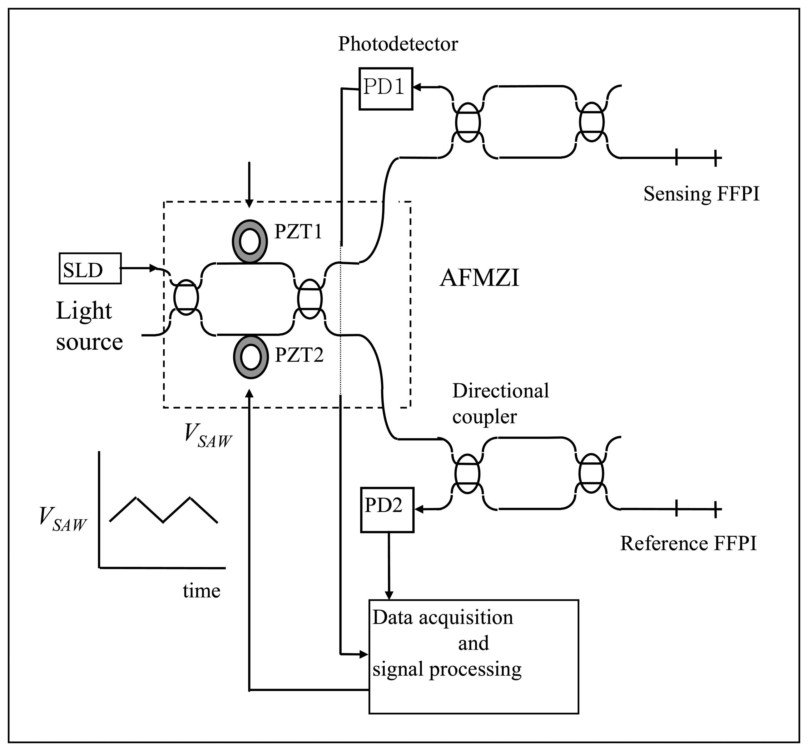
From the beginning of this research, an all fiber white light interferometry (AFWLI) absolute temperature measurement system as shown in
Figure 1 was selected as the application area of the proposed signal processing algorithm. White light interferometry departs from the conventional interferometry in that it uses a broadband light source. SLD in
Figure 1 represents a superluminescent diode (SLD) used as a broadband light source and PD1, PD2 denote photodetectors 1 and 2, respectively. In the AFWLI two fiber Fabry-Perot interferometers (FFPI, sensing FFPI and reference FFPI in
Figure 1) and a Mach-Zehnder Interferometer as a processing interferometer (scanning interferometer in
Figure 1, hereafter termed as MZI), which has two piezoelectric transducers (hereafter termed as PZT) in its two arms, are connected in tandem. The sensing and the reference interferometer output signals from PD1 (
Equation 1 for PD1) and PD2 (
Equation 2 for PD2) are given respectively by:
where
LC is the coherence length of light source, Φ
P is the OPD (Optical Path-length Difference) between two arms of Mach-Zehnder processing interferometer and Φ
S, Φ
R are the round trip phase shifts for the sensing and reference FFPIs, respectively. In
Equation 1 and
Equation 2 it is assumed that light source has a Gaussian power spectrum. A constant d.c. voltage
VDC (100∼150 volt,
Figure 1) is applied to the PZT1 in one arm to coarsely match the OPD of the MZI to that of the sensing FFPI. And an alternating ramp voltage
VSAW (
Figure 1) is applied to PZT2 in the other arm to scan the processing interferometer so that OPD Φ
P between two arms of MZI can be varied over a certain range.
This AFWLI for temperature measurement produces two fringe scans, one from the sensing FFPI and another one from the reference FFPI, as shown
Figure 2. In AFWLI, the sensing FFPI is exposed to the temperature
TS to be measured and the reference FFPI is protected from environmental disturbances but exposed to the known reference temperature
TR. Now, assume that the known temperature of the sensing FFPI and the reference FFPI are
TS and
TR, respectively. When the phase Φ
P of MZI is scanned and exactly matched to that of the sensing FFPI (the reference FFPI), a zero order fringe peak of the sensing FFPI (the reference FFPI) is produced at certain Φ
P = Φ
P,S (Φ
P = Φ
P,R), as shown in
Figure 2. In
Figure 2, Φ
P,S (Φ
P,R) denotes the phase of the processing interferometer producing the zero order fringe peak of the sensing FFPI (the reference FFPI). If we can identify the phase difference Φ
d = Φ
P,S – Φ
P,R (this is possible by the proposed signal processing algorithm which will be shown later in this article) then Φ
d is mapped to the temperature
TS and absolute temperature measurement is possible. This problem has been known as “Time Delay Estimation (TDE) [
3] (or Phase Delay Estimation)”. In this article, a new signal processing algorithm to estimate the phase delay Φ
d of AFWLI is proposed. This article consists of five sections. Section 2 describes the previous related works for time delay estimation methods. In Section 3, a signal processing algorithm to measure the phase difference Φ
d of AFWLI is proposed. In Section 4 the performance of the proposed signal processing algorithm has been demonstrated using computer simulations. Section 5 shows the comparison to the previous literature and Section 6 is the conclusion of this article.
2. Previous works
Two major classes of signal processing algorithms for WLI are the hardware approach and the software approach. Both approaches have a more or less “tracking zero order fringe peak” feature. Gerges proposed a hardware approach which locks the zero order fringe position of interferometer by a feedback loop [
4]. An improvement of the sensitivity up to 1/240 fringe was claimed. To the author's best knowledge this method, while still dependent on the incremental characteristic of laser interferometry and not fully taking advantage of WLI's potential to identify the interference fringe, demonstrated the feasibility of locking and tracking the fringe peak for absolute measurement for the first time.
There are many software algorithms to estimate phase delay Φ
d [
3,
5]. Among many detection methods, the cross-correlation method dominates the field of phase delay estimation in practice due to its easier implementation [
6]. Many other TDE methods are based on this algorithm. The cross-correlation method cross-correlates the two fringe signals
iS(
n) and
iR(
n), which are sampled versions of
IS(Φ
P) and
IR(Φ
P) respectively, into
i(
n) and considers the sample number argument
n=
nd that corresponds to the maximum peak in cross-correlation
i(
n) as the estimated time delay [
7].
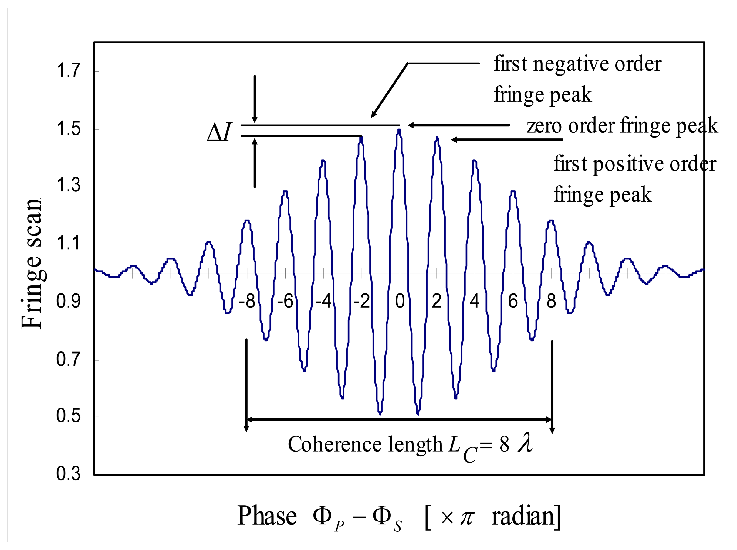
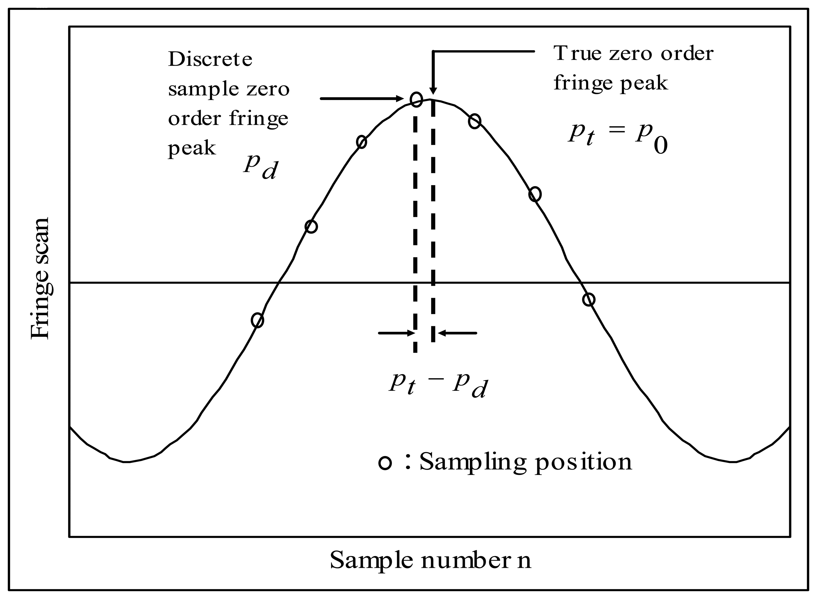
While WLI has the potential to identify the interference fringe order from the output pattern of an interferometer [
8], it is difficult to distinguish the zero order fringe peak from its adjacent first order fringe peaks when noise is present in the interferometer output, as shown in
Figure 3. From
Equations 1 and
2, the amplitude difference Δ
I between the zero order fringe peak and the first order fringe peaks is represented as:
Clearly, if a system has a noise level which is equal or greater than Δ
I the zero order fringe peak cannot be identified directly, simply through inspection of its amplitude. If the normalized zero order fringe peak value is defined as unit signal, a minimum signal-to-noise ratio
SNRmin required to identify the zero order fringe peak [
9] is given by
Representative values of the coherence length of different light sources like white light lamp, light emitting diode (LED), superluminescent diode (SLD), are about 10, 20, and 40 in terms of optical fringes. The
SNRmin required to identify the zero order fringe peak by amplitude difference Δ
I is given from
Equation 3 as 28 dB, 40 dB, and 52 dB respectively [
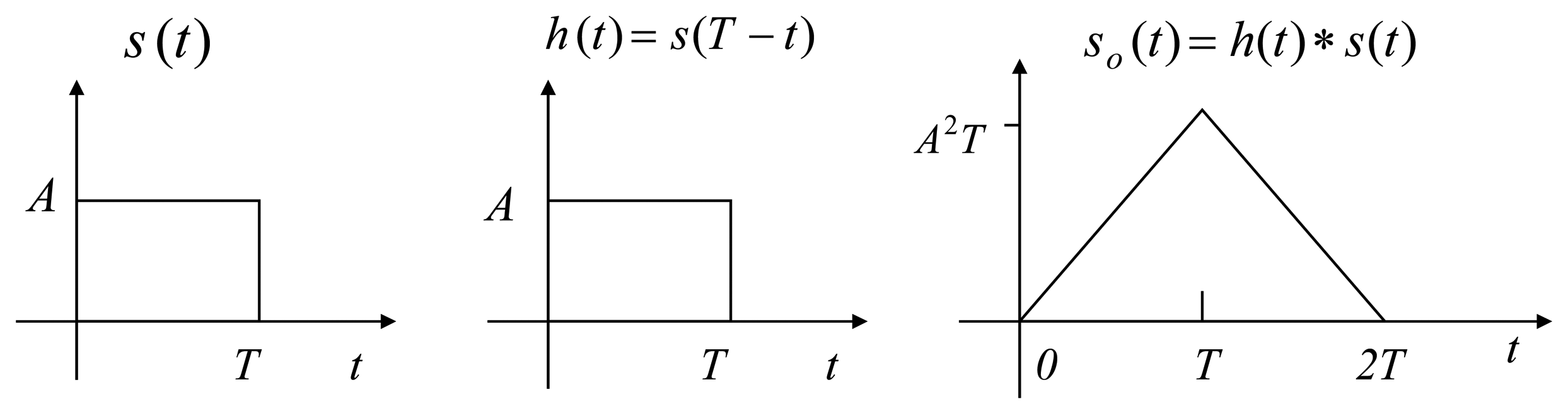
9]. One disadvantage related to cross-correlation is the broadening of envelope (or peak) (hereafter termed as envelope) from
LC to
due to the cross-correlation of two almost identical Gaussian envelope signals [
17]. This results in higher
SNRmin in
Equation 3 requiring 6 dB more than before cross correlation. Then, with this broadening, the attainable resolution is often not better than one fringe and a precise peak location may be somewhat questionable. This difficulty has inhibited the application of fiber optic sensors using WLI, for example, absolute OPD determination [
9].
Additionally, once the zero order fringe peak is identified, then for a more accurate sub-sample resolution time delay estimation we will have to use interpolation which is possible by either quadratic interpolation in time domain or frequency domain zero-padding [
10,
11]. But quadratic interpolation uses three cross-correlation values centered at the estimated peak of cross-correlation. This method has a shortcoming of bias caused by time domain sample rate [
12,
13] and the difference between true peak shape and the fitted quadratic polynomial. In frequency domain zero-padding, the number of zeros are padded in the middle of Fourier Transform of cross-correlation
i(
n). Notice that zero-padding in frequency domain increases the discrete frequency by a certain factor which eventually results in time-domain interpolation in cross-correlation signal
i(
n). Zero-padding in frequency domain is a useful tool to improve the peak location accuracy, but it increases the computational complexity [
14] and storage requirement associated with inverse Fast Fourier Transform (FFT) operations [
15].
Notwithstanding the above mentioned shortcomings, cross-correlation is a still useful tool for time delay estimation as shown that cross-correlation with no pre-filtering is an optimal maximum likelihood estimator to estimate the time delay between two similar signals if the noise processes
wR(
n),
wS (
n) of signal
iR (
n),
iS (
n) are white noises and at least one of signals has high signal-to-noise ratio greater than 10 dB [
16].
The outcome of the time delay estimation depends on the combined performance of coarse estimation (zero order fringe peak identification) and sub-sample resolution estimation of time delay. In this article, a new signal processing algorithm which can accurately identify the zero order fringe peak of cross-correlation i(n) of two fringe scan output signals of a WLI is proposed. This algorithm still uses a cross-correlation technique taking advantage of simple implementation. But this algorithm combines the hypothesis test as a coarse estimation to reduce the possibility of mis-identification of peak with fine tuning algorithm as a sub-sample resolution peak estimation to overcome the shortcomings of quadratic interpolation or frequency domain zero-padding.
The proposed signal processing algorithm uses a software approach, which is potentially inexpensive, simple and fast. And, this proposed signal processing algorithm has a low peak mis-identification rate of 3 × 10⁻⁴ at 31 dB SNR and has a high precision fine tuning capability down to 5 × 10⁻⁴ fringe as will be shown from the computer simulation results.
4. Computer Simulations
The proposed signal processing algorithm was verified using computer simulations. To see the shot-noise limited performance of the proposed signal processing algorithm, the normalized AFWLI fringe scans,
iS(
n) and
iR(
n) were computer-generated using
Equation 4 and
Equation 5 respectively and shot noise was added to the AFWLI fringe scans,
iS(
n) and
iR(
n) instead of white noise. In the computer simulations the zero order fringe peak position
p0,S (and
p0,R) for
iS(
n) (and
iR(
n)) were randomly selected as real number.
iS(
n) and
iR(
n) were cross-correlated into
i(
n). Then,
pt is calculated as (
p0,S-
p0R) and zero order fringe peak
pd =
nd of
i(
n) becomes the integer part of
pt. The coherence length of
iS(
n) and
iR(
n) were chosen as
LC=26
λ to simulate the coherence length of the commercially available SLD like OKI OE350S from Oki semiconductor. For all the computer simulations presented in this article parameters are fixed as follows, unless the specified parameter is varied for a certain range and circumflex notation ∧ on the top of the parameter denotes the estimated value of that particular parameter calculated by the proposed signal processing algorithm.
Sample rate fS =16 [samples/fringe]
SNR=30 dB
Effective Coherence length
Size of fine tuning step Δn=1/1000 [fringe]
4.1. Simulation: Miss rate simulation
In the first simulation miss rate (misidentification rate) of the proposed signal processing algorithm was tested at different shot noise levels. The
SNR was varied from 1 dB to 28 dB with 1 dB separation and a set of 10000 simulations was carried out at different
SNR. When the position difference between the estimated zero order fringe peak
p̂d and the computer-generated zero order fringe peak
pd is bigger than half fringe (8 samples), the zero order fringe peak is considered to have been misidentified.
Table 2 shows the miss rate of the proposed signal processing algorithm and miss rate is defined as the ratio of number of miss to 10000.
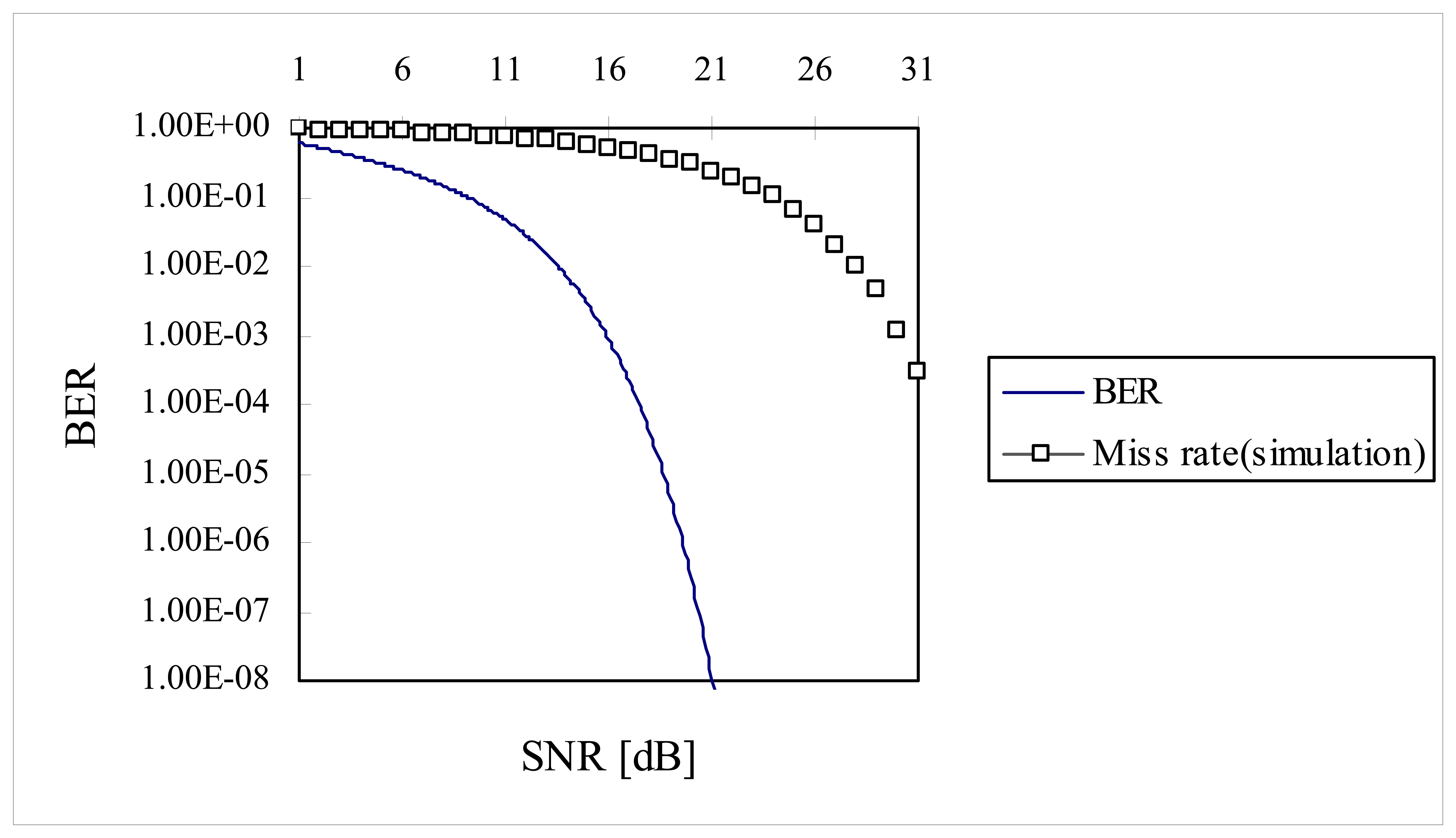
In
Figure 9, miss rate was plotted along with Bit Error Rate (BER) of binary fiber optic communication system [
19]. In
Figure 9 (or
Table 2) we have a rule of thumb that every dB improvement in
SNR (over the range of 26 ∼ 31 dB) produces approximately one order of magnitude improvement in error rate. This kind of behavior is also the case for binary fiber optic communication system (two orders of magnitude improvement in error rate for the binary fiber optic communication system).
To extrapolate the miss rate beyond the range of 10
-4 on the BER curve, data points in abscissa in
Figure 9 were left-shifted by ∼14.2 dB (by trial and error) until data points of miss rate between 16 dB ∼ 31 dB were visually fitted on the BER curve. Then four more data points were extrapolated beyond the data point of miss rate at 31 dB
SNR on the BER curve as shown in
Figure 10. It is predicted that miss rate will be 3 × 10
-8 at
SNR of 35 dB.
4.2. Simulation: Root mean square (RMS) error of the zero order fringe peak identification
After the zero order fringe peak was identified, fine tuning was calculated for resolution enhancement. Phase error Φerror,i between computer generated zero order fringe peak pt (or p0) and fine-tuned zero order fringe peak p̂t (or p̂0) was calculated. Phase error Φerror,i was averaged over 30 simulations at a given SNR and this average gives out the root mean square (RMS) error of the zero order fringe peak identification.
Figure 11 shows the change of RMS error along with the
SNR in the range of 10 dB to 40 dB and
Figure 12 shows the change of RMS error along with the
SNR in the range of 30 dB to 40 dB. It is shown that the minimum
SNR required to achieve RMS error less than 10
-3 [fringe] (which is the fine tuning step size) must be greater than 35 dB
SNR.
4.4. Simulation: Effects of b̂ (f̂S)
In this simulation, estimated effective coherence length
L̂C,eff was set as 36 fringes,
SNR=30 dB and estimation error of the zero crossing period
b̂ was varied from -10% to 10% when
b=10 (
fS =20 samples/fringe) to see the effect of estimation error of the zero crossing period
b̂ on the performance of the proposed signal processing algorithm. The estimation error of the zero crossing period
b is defined by:
where
b is the half the sample rate
fS. In
Figure 14, it can be shown that RMS error of fine tuning was not sensitive to the estimation error of
b̂ within the range of ±6% estimation error of
b and especially, RMS error of 0.001 [fringe] was obtained within the range of 2% estimation error of
b. But, on the range of ±7% ∼ ±10% estimation error
b̂ RMS error increased dramatically to 0.25 fringe.
This is presumably due to the fact that
i(
n) and test cross-correlation
itest(
n) (
Equation 24 or
Equation 25) started to be out of phase and RMS error increased fast.
4.5. Simulation: Effects of L̂C
This simulation is to show the effect of estimated coherence length
L̂C on RMS error assuming that
b̂ =
b, LC=26λ(
LC,eff ≈ 36λ) and
SNR was fixed as 30 dB. Estimated coherence length
L̂C was varied from 21λ to 30λ. In other words, estimated effective coherence length
L̂C,eff was varied from 30λ to 42λ and RMS error was observed.
Figure 15 shows that RMS error turned out to be not sensitive to the estimation error in coherence length
L̂C,eff. This is due to the property of cross-correlation. Cross-correlation is maximized when
pt and
pd +
MΔ
n are in phase as long as both cross-correlation
i(
n) and test cross-correlation
itest (
n) are symmetric.
5. Comparison to the literature
In this section a comparison to the previous literature data regarding the resolution of zero order fringe peak detection is given. Interestingly enough, reference [
20] calculated the theoretical limit of scanning white light interferometry signal evaluation algorithm. In this reference the theoretical limit of resolution of the fringe order detection was given as:
where
Si=
S(zi) consists of a fixed number of intensity values, typically taken at equidistant positions
zi,
I(
z) is the ideal input signal (i.e. fringe scan) to be subject to intensity noise
N(
z),
zc of
I(
z) is the position to be found using the evaluation algorithm (signal processing algorithm). And it is assumed that intensity noise
N(
z) is the constant noise value
N over all samples. In our case, cross-correlation
i(
n) can be represented as the generalized equation as follows again:
Then, the derivative of
i(
n) becomes:
and (
i′(
z))
2 is given as:
As can be seen from the
Equation 34, theoretical limit of fringe order detection is the function of sample rate, effective coherence length and
SNR. Theoretical limit of resolution for the computer simulation shown in
Figure 11 and
Figure 12 can be calculated using the parameters of 16 sample per fringe (Δ
z= λ/16), effective coherence length
. Then theoretical limit of resolution of zero order fringe detection in
Figure 11 and
Figure 12 is given as:
Figures 16 and
17 are the comparison of the computer simulation results and the theoretical limit of fringe order detection calculated by
Equation 35 and
Equation 36. As shown in
Figure 16, computer simulation results produce a much bigger RMS error than the theoretical limit over low
SNR range (10∼30 [dB]). In comparison to the literature, it seems like that theoretical limit of reference [
20] is more optimistic over low
SNR range than the computer simulation performance. But, the proposed signal processing algorithm has proven to reach the theoretical limit of fringe order detection over the higher
SNR range (30∼40 [dB]). This is not a surprising result because in higher
SNR fine tuning algorithm will enhance the fringe order detection resolution down to the theoretical limit once zero order fringe peak is identified correctly. But, over low
SNR range, fine tuning algorithm is not effective in enhancing the fringe order detection resolution because probably zero order fringe peak is misidentified and fine tuning is searched within the half sample of the misidentified zero order fringe peak.
Increasing the fine tuning range will help to locate the zero order fringe peak correctly and lower the RMS error down to the theoretical limit, although this is time consuming. Optimum fine tuning range of M over low SNR range to find the correct zero order fringe peak will be the subject of further research.
6. Conclusions
A new signal processing algorithm for white light interferometry has been proposed. The goal of signal processing algorithm was to find the time delay (phase shift) between two fringe scans which makes it possible to measure the absolute optical path length of a sensing interferometer. This new signal processing algorithm can be used for absolute temperature measure measurement by mapping the zero order fringe peak position of cross-correlation
i(
n) to the time delay between two fringe scan. Cross-correlation between two fringe scans utilizes all the photons in fringe scans effectively and the uncertainty of the zero order fringe peak mis-identification was reduced. Monte-Carlo simulations showed that the proposed signal processing algorithm identified the zero order fringe peak with a miss rate of 3×10
-4 at 31 dB shot noise and the extrapolated miss rate at 35 dB shot noise was 3×10
-8. Also resolution of less than 10
-3 fringe was obtained at 35 dB shot noise (
Figure 12). The fine tuning of signal processing algorithm requires some prior knowledge on the coherence length
LC of the SLD and sample rate
fS. But the performance of proposed signal processing algorithm turned out to be not sensitive to the estimation error in
L̂C and
f̂S (within the range from −6% to 6% estimation error of
b̂). Also the proposed signal processing reached the theoretical limit of fringe order detection over the higher
SNR range (30∼40 [dB]). The proposed signal processing algorithm uses a software approach which is potentially inexpensive, simple and fast. As a whole, the proposed signal processing algorithm has proven to be a high precision signal processing algorithm for AFWLI phase (time) delay estimation.


