A laboratory model of the digital sun sensor implementing the enhanced, multi-hole configuration has been realized by the authors with the aim of characterizing the enhanced configuration and assessing its performance with respect to the basic one (i.e. the one-hole configuration), developing and testing algorithms for system operation, operating and testing COTS solutions for the MSS flight unit in view of the MIOsat mission.
3.1. Hardware Model
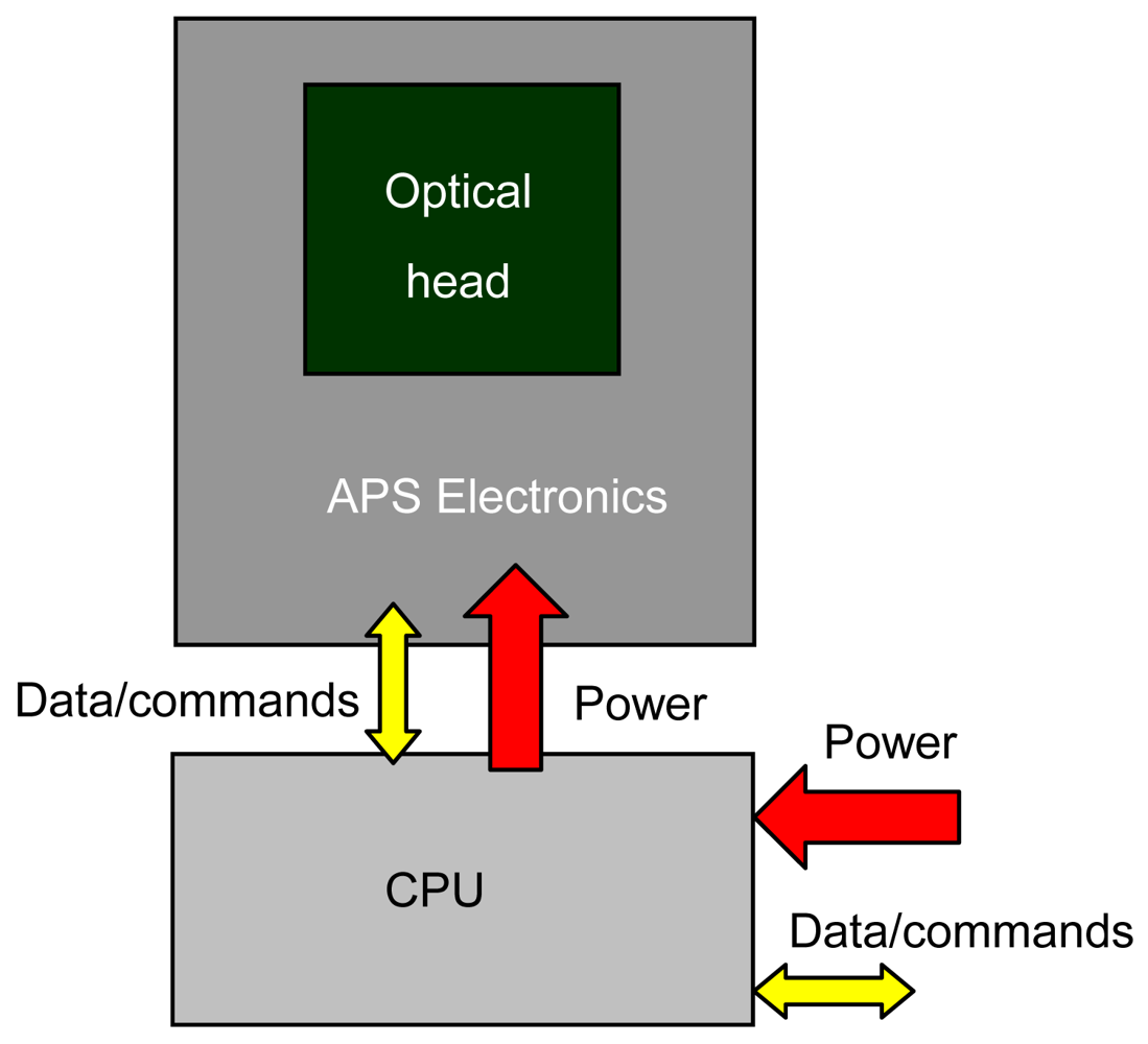
A sensor architecture consisting of two distinct hardware units (see
Figure 2), corresponding to its two functional units, OH and CPU, is selected for the model to get on-board installation flexibility for the flight validation.
Based on the objectives of the MSS experiment within MIOsat program, sensor components are defined by selecting COTS parts for both the OH and the CPU. Parts not available on the market, like the mask, are designed and realized specifically, making use of standard materials and manufacturing processes as far as possible. It is worth noting that the current sensor model, which is the evolution of a previous prototype [
9-
11], is intended mainly as a proof of concept, i.e. it is developed with the main intent of testing on ground, and, then, in flight, innovative concepts and solutions for the optical head, as well as calibration and processing algorithms. For this reason, the sensor design it is not optimized in terms of miniaturization of some of its components.
The OH includes the CMOS photodetector, the focal plane electronics and the mask. The photodetector is a two-dimensional CMOS Active Pixel Sensor (APS) produced by Micron Technology Inc.™. This unit includes a 10-bit ADC, programmable electronics for some basic camera functions (i.e. shutter time setting, windowing, row/column skipping), and part of the focal plane electronics. Focal plane electronics and I/O interface to the CPU are implemented in two commercial boards, also by Micron. The board containing the detector implements all the needed focal plane circuitry for detector control and image acquisition, whilst the other board operates conversion of the detector specific communication protocol to the USB 2.0 standard.
As previously specified, the opaque mask was designed in house by the authors. It is manufactured out of a very thin, plain steel foil, and the required holes are realized by electron discharge, a low-cost, micro-manufacturing process that allows precision up to 0.01 mm in hole size and shape. It is worth noting that the use of such a metal foil for the mask, being its thickness comparable to the hole size, determines that imaged spots are distorted as the sun-line gets far from the sensor boresight. However, it represents a systematic effect that can be completely compensated for, at least theoretically, by the Calibration Function (CF). Nevertheless, for increasing off-boresight angles, summed to the reduced irradiance toward the focal plane, it reduces the acquired image quality. For the flight unit, an aperture protection filter will be added to the mask, so that the solar radiation reaching the focal plane will not saturate the photodetector also thanks to proper shutter time setting. Filter and shutter time will be tuned to keep sun-spot pixel signals within 70 % of full scale, and to allow for the desired output rate. By doing so, when celestial bodies other than the sun are in the sensor FOV during real operation, their radiation reaching the focal plane will only generate signals within the image noise already present, being the sun much brighter (e.g., > 420,000 times than full moon and 30,000 times than earth albedo).
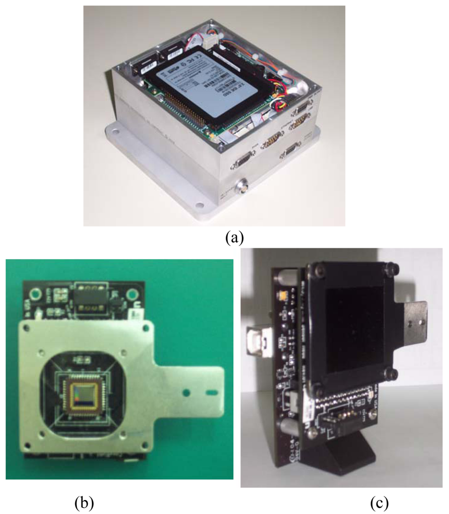
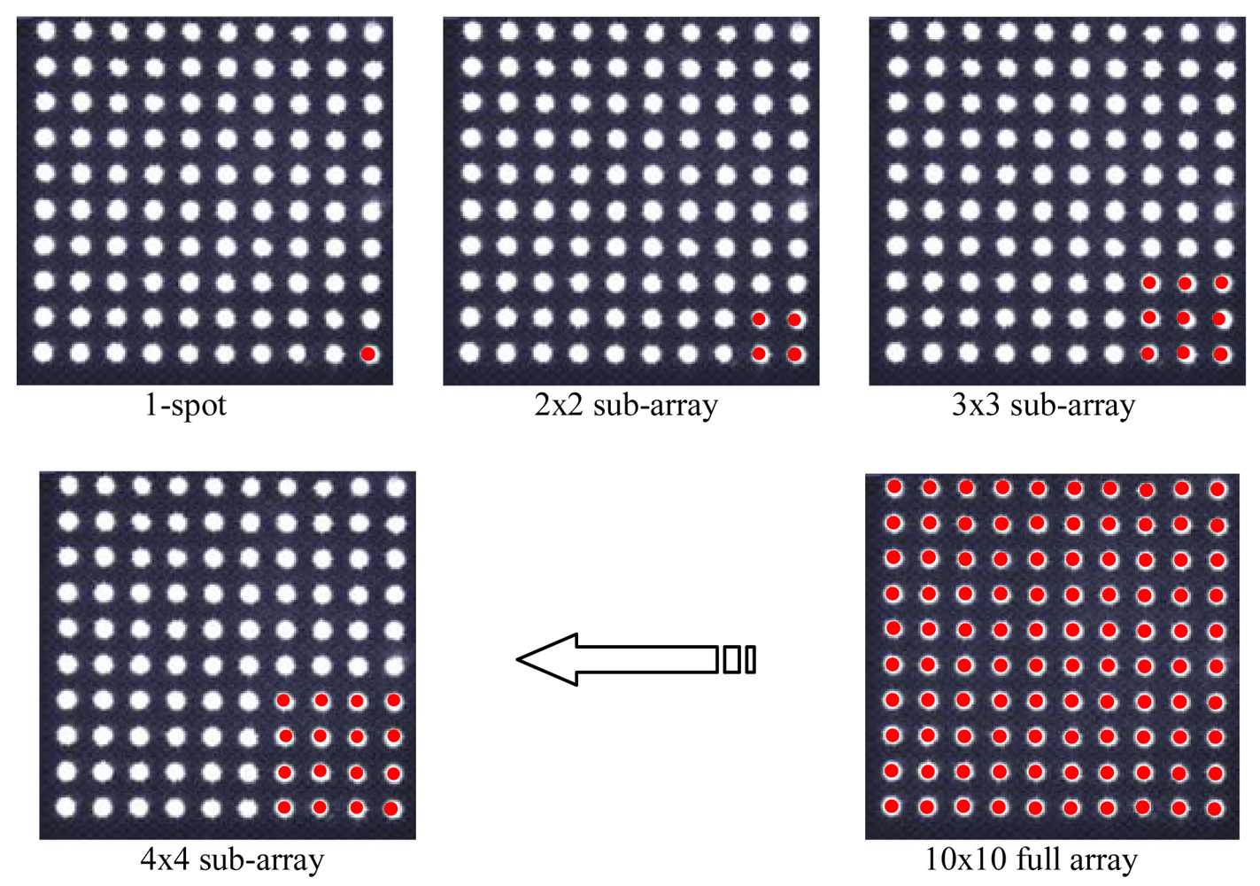
To test both basic and enhanced sensor configurations, two different masks are realized, with one and 100 holes, respectively, arranged in a 10 × 10 array. Hole size is the same (0.1-mm radius) in both cases, which determines imaged spots with diameter of about 60 pixels for the adopted detector. A mechanical interface (mask holder, see
Figure 3) is designed and realized ad hoc to couple the focal plane to the mask, in accordance with the nominal design configuration, in which mask and detector sensing surface are parallel, at a distance equal to the focal length, and their centers are aligned so that the resulting FOV is symmetrical with respect to the boresight axis. The mask adapter also includes a support for the sensor installation in the test facility.
Figure 3 shows pictures of the two sensor functional units. Specifically,
Figure 3(b) shows the sensor board and the mask holder adopted for sensor testing in the laboratory test facility.
Table 1 reports the OH nominal technical characteristics.
The CPU is a single-board computer in pc-104 format by RTD™. It is a COTS product designed for operation in harsh environment (i.e. extended temperature, conduction-based cooling). It includes all the needed peripherals and interface in a single board, and it is also equipped with a pc-104 power-conditioning module to regulate the power input from the unregulated bus and to supply both the CPU and the OH. The latter one, in particular, is powered by the CPU at 5 Vdc via the USB link, which is also used for CPU-OH data exchange.
A solid state mass memory is adopted to get reliability of operation in space. Accurate analyses are being carried out for both the CPU and the OH electronics to assess critical technologies for space operations, so to identify viable solutions to guarantee the reliability and lifetime needed for the experiment execution and goals. In this context, typical space environment problems (i.e. radiation, vacuum, thermal) are being addressed. In particular, space radiation shielding adequate for a two-years lifetime will be guaranteed by specifically designed, aluminum enclosures (see
Figure 3). Preliminary mass and power budgets of the sensor model are reported in
Table 2. It is worth noting again that mass and power consumption values refer to the commercial units adopted for the sensor prototype development to allow proof of concept on ground and in flight.
3.2. Software Model
It includes the routines for sensor operation management, image acquisitions, I/O to the satellite OBDH, and the routines implementing the algorithms for sun line determination. These algorithms, which are the topic of the next sub-sections, basically consist of image processing algorithms, to evaluate the FP position of the sun image(s), and calibration algorithms, which use position information to extract the sun line orientation:
Image processing algorithm basically perform image preprocessing, such as noise reduction, and computation of the FP position of the spot-like sun image(s). Specifically, once the spot has been localized to pixel accuracy, its sub-pixel position is computed as the centroid of the multi-pixel image as [
15]:
where x
c and y
c are the centroid FP co-ordinates, x
k and y
k are the FP co-ordinates and I
k is the intensity of the generic pixel in the considered n-pixel integration window (including the whole spot). Of course, centroiding of
Equation (2) is applied after some image pre-processing, that is noise removal, spot search and rough localization necessary to select the contriding integration window. Details about the adopted algorithms and the error sources affecting centroid determination can be found in [
9-
11].
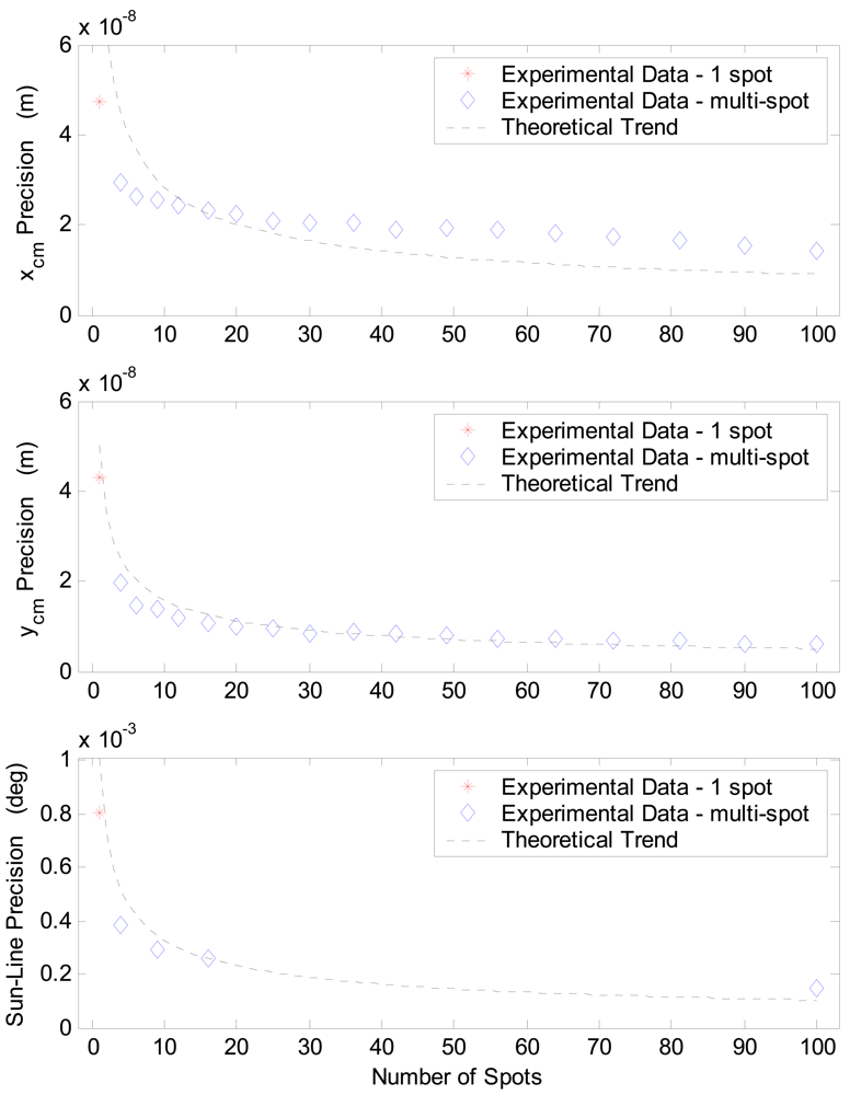
The above processing does not need any particular specialization when applied to the multi-spot configuration. Indeed, in this case an array of spots must be imaged and processed. Preliminarily, the whole array is localized on the FP and its size is checked out to verify if it is only partly imaged due to a large off-boresight of the sun or any acquisition problem. Then, a centroid should be computed for each of the spots to produce multiple estimates of the same illumination direction, which should be then averaged to get highly precise sun line determination. Nevertheless, such a strategy would require the management of a large number of sun-line computations. Indeed, a dedicated CF would be needed for each spot of the array, i.e., a dedicated function should be constructed after calibration tests, implemented in the on-board software, and run at the time of sensor operation. The latter two aspects are particularly critical, since they impact flight-unit design and operation leading to more demanding requirements. To overcome these critical aspects of the enhanced configuration operation, the averaging is carried out at the stage of centroid computation. Hence, a centroid is computed for each imaged sun spot and, then, they are averaged to extract an average centroid. The latter one is dealt with as the single-spot centroid of the basic sensor configuration. In this way, the additional computational load required by the multi-hole configuration is limited to the computation of multiple centroids.
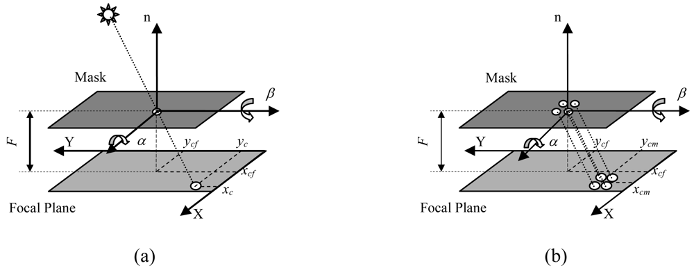
The CF maps the sun spot computed FP position into the sun line orientation, which is described by the two angles α and β in
Figure 1. They represent the sequence of rotations needed to align the sensor boresight axis with the illumination direction.
The authors have considered and tested several solutions to implement the mapping function [
11], aiming at achieving computational efficiency in terms of simplicity, by requiring neither numerous parameters nor complex computations, and accuracy over the whole sensor FOV. Very simple schemes based on the following basic geometrical model:
were tried, showing poor accuracy, especially for large sun-line off-boresight angles. Indeed, the geometrical model in
Equation (3) does not take account of unavoidable misalignments of sensor components and, more in general, deviations from the design nominal configuration. In addition, only scarce improvements are achieved by using more complex geometrical models in which additional parameters are introduced to model the actual mask-FP geometry (i.e. focal length and component misalignments) estimated during sensor calibration by LSQ best fit. In fact, additional non-linear effects are present, due to mask thickness, manufacturing tolerances, diffraction effects, non-uniform response and finite size of photodetector pixels, which cannot be explicitly included in the model. Hence, in spite of the poor results, there would be a significant increase in the complexity of the model which impacts negatively both the calibration procedure and sensor operation.
Neural-network-based CFs provide a viable and interesting alternative solution to achieve high accuracy without introducing very complex models. Indeed, Neural Networks (NNs) with supervised training are universal approximators, i.e., they can approximate to any desired degree of accuracy any real-valued, continuous function (or
sufficiently regular function, with a countable number of discontinuities between two compact sets). Moreover, NNs, if non-linear w.r.t. their parameters, are also parsimonious, that is they implement the desired approximation using the lowest number of parameters [
16,
17]. Hence, they can be effectively exploited to build the CF, since they can implement the required mapping without any prior assumption about the centroid-to-sun-line transformation, by constructing the non-linear mapping on the basis of experimental data only.
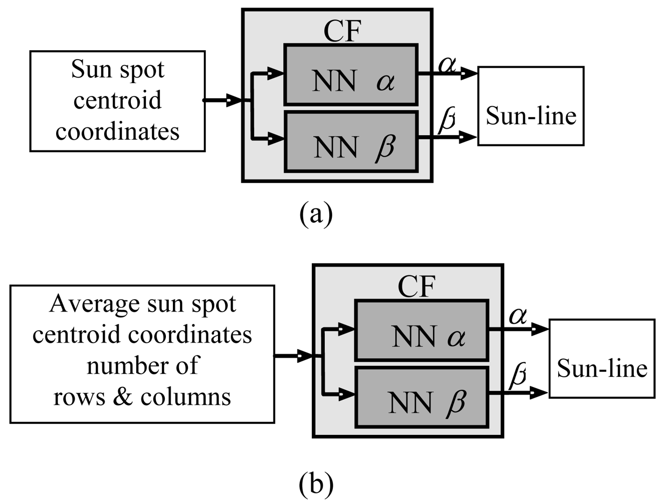
Multilayer feed-forward NNs with sigmoid activation function in the hidden layer and linear output neurons are considered for this application. In particular, the selected NN structure consists of one hidden layer. Different NN architectures characterized by a different number of neurons in the hidden layer have been tested. Two distinct NNs are used to compute α and β independently. Several solutions (see
Table 3) in terms of NN input/output variables were compared in previous, dedicated test campaigns [
11]. Specifically, fully-neural CFs were built and compared to mixed models in which neural corrections were introduced to refine results of the geometrical models. It was found out that the most satisfactory trade-off is represented by the scheme in
Figure 4(a), which shows the lighter computational load and very good accuracy on a wide FOV. It is worth mentioning that the number of neurons in the hidden layer cannot be uniquely fixed, but it is peculiar to each case and has to be determined during calibration.
The FOV size in the basic operation mode, referred to as Standard FOV (S-FOV) in the following, is reduced during operation with multiple sun spots by the requirement that all the imaged spots lie within the detector sensing area. Hence, for a given detector, using a large number of sun images improves sensor precision at the cost of reducing the measurable range of off-boresight illumination directions. The theoretical FOV size of the UniNa MSS prototype is in the order of 40 × 20 [
10] for the mask with a 10 × 10-array of holes. It is worth noting that size and aspect ratio of the sensor FOV are determined by the sizes of the detector sensing area and of the imaged array of spots. Hence, even for a given detector, FOV size and aspect ratio can be customized by modifying the array of holes on the mask, in terms of number, size and arrangement of the holes.
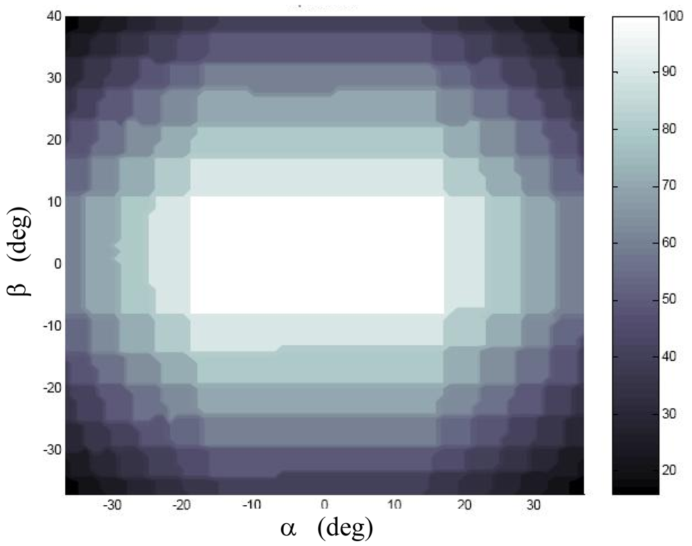
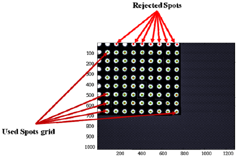
It is possible to widen the range of measurable illumination directions by accepting that a reduced number of spots lies within the detector sensing area (eXtended FOV, X-FOV). By doing so, the computation of the sun-line is based on a variable number of spots. In particular, the larger the off-boresight angle is, the lower the number of usable spots gets. This fact determines a reduced precision at the FOV edges because of the lower number of simultaneous measurements that can be averaged to produce the final result. Also a new calibration function must be implemented, valid over the whole useful X-FOV and capable of accounting for the variable number of exploited sun spots. Of course this calibration function should not introduce any performance loss at the X-FOV center.
The above described X-FOV mode is implemented in the sensor prototype and tested on ground. To this aim, also an enhanced centroiding algorithm is developed. It computes the average centroid of a set of sun spots arranged in a two-dimensional array, assuming that the number of rows and columns can be variable. For the calibration function, the same neural structure of the S-FOV mode was maintained. However, the NN input stage is modified so to exploit also the imaged spot array size (i.e. row and columns) to map the average centroid into the illumination direction (see
Figure 4b). In the X-FOV operating mode, the sensor gets a theoretical FOV larger than 80 × 70 [
18].
Figure 5 shows the number of correctly imaged spots in the extended FOV, as obtained in laboratory tests.


