Bayesian Statistics for Loan Default

Abstract

Bayesian inference has gained popularity in the last half of the twentieth century thanks to the wider applications in numerous fields such as economics, finance, physics, engineering, life sciences, environmental studies, and so forth. In this paper, we studied some key benefits of Bayesian inference and how they can be used in predicting loan default in the banking sector. Various traditional classification techniques are also presented to draw comparisons primarily in terms of the ease of interpretability and model performance. This paper includes the use of non-informative priors to attempt to arrive to the convergence of posterior distribution. Finally, with the Bayesian techniques proven to be an alternative to the classical approaches, the paper attempted to demonstrate that Bayesian techniques are indeed powerful in financial data analytics and applications.

1. Introduction

For the past centuries, the most dominant philosophy in statistical inference is frequentism, and in a large part, it is still the case today. Frequentism assumes that the unknown parameter is a fixed quantity and is based only on the information on the sampling data without injecting any prior knowledge.

In contrast, Bayesian inference (Fornacon-Wood et al. 2022) adopts a different philosophy. However, The key difference is that although both philosophies use likelihood (data), only Bayesian uses prior information. Bayesian is based on an approach in that both the data and parameters are considered as probability distributions. All current knowledge regarding data and parameters is summarised in the probability distributions. Based on the likelihood function (data), the prior knowledge is updated to produce a posterior distribution. The differences (Fornacon-Wood et al. 2022) between the two approaches are well-documented.

Although the Bayesian theorem was first introduced in the 18th century by Thomas Bayes, it did not garner attention until the 1950s and 1960s. The primary reason for the slow adoption of the Bayesian method was the lack of computational power coupled with contemporary software as Bayesian implementation requires intensive resources to produce the posterior distribution. The lack of the adoption of Bayesian inference, especially amongst frequentism, is due to the use of prior information, which is considered by many to be subjective, even though it can be based on historical events or inputs from subject experts. Bayesian has been frowned upon due to the subjective nature of priors (Gelman 2008). In fact, the Bayesian method is found to be based on the subjective interpretation of probability.

The present study is of interest as the loan performance has a direct impact on the overall well-being of banking institutes. As important as the ‘credit culture’ and ‘risk management capabilities’ have on the lending institutes, institutes with the best credit ratings—Lehman Brothers, etc.—still failed and subsequently collapsed. Borison (2010) argued that the fundamental difference was in the practice, where a non-Bayesian approach was primarily used for credit risk assessment. The downfall of frequentism was highlighted by Borison et al., while on the other hand, the distinct advantages of Bayesian were highlighted. For example, it was mentioned that traditional risk management adopts the frequentist approach with three well-known and inherent shortcomings as follows:

• The frequentist view places excessive reliance on historical data, which may lead to poor performance should the historical data be lacking or misleading;
• The frequentist view provides little-to-no incorporation of knowledge and experience to build sound judgement. In other words, proven prior knowledge and experience are not included;
• The frequentist view instils a false sense of security, which leads to a sense of complacency as it encourages a heavy reliance on actions that are supposedly based on scientific truth, however, in reality, many of the most critical and riskiest decisions do not sit within the narrow frequentist paradigm.

This study was also confirmed by the findings in numerous publications such as Berg et al. (1992), Zago and Dongili (2006), and most notably, the work by Berger and DeYoung (1997). First, Berg et al. and Dongili et al. both documented and confirmed that toxic or bad loans had a negative correlation with the health and performance of banking institutes. Berg et al. further confirmed that good loans underpinned by good corporate governance provides the platform for efficient performance in the banking sector. Berger et al. also found a negative relationship between the cost efficiency and credit quality measured by non-performing loans (NPL), and concluded that banking institutes with higher NPLs incurred higher costs and were less profitable than banks that addressed best practice through the implementation of better governance. Therefore, it is of the utmost concern for banking institutes to only issue loans that are high performing by minimizing bad loans through data driven classification.

Recently, Bayesian has been used in financial and risk applications because of its proven applications in many fields including its ability in predicting bad loans. For example, Bijak and Thomas (2015) modelled the loss given default (LGD)—the loss borne by lending institutes—using the Bayesian hierarchical model and produces posterior means of parameters that resemble that of a frequentist approach. Smith and Elkan (2004) instead employed a Bayesian approach to include reject applicants in the training set in order to create an unbiased prior. Wang et al. (2020) used both frequentist and Bayesian methods for parameter estimation and default rate stress testing by modelling the uncertainties of the coefficients to reduce credit risk underestimation.

The study is needed as it focuses on the repeatability and validity aspects of deploying the Bayesian method in modern scenarios with use of a contemporary approach:

• We present a case study that Bayesian is important and can be an alternative to the frequentist approach in predicting loan default;
• We illustrate the repeatability and validity of deploying an analytics life cycle with the use of contemporary software packages. Data for the training are randomly obtained with no leakage or biasness;
• We first perform the comparisons of classical logistic regression and traditional machine learning methods to Bayesian;
• Finally, we extend the model performance and convergence comparisons to various distributions for non-informative priors.

Therefore, the study aimed to explore the use of Bayesian inference to determine whether the loan applicant has the propensity to default. Traditional approaches such as classical logistic regression, support vector machine, gradient boosting machine, random forest, and others have been used to draw comparisons between the model performance and other factors such as the ease of interpretability as one of the greatest advantages of Bayesian lies in its interpretability.

The rest of this paper is organised as follows:

• In Section 2, we briefly cover the background of the Bayesian technique and how Bayesian has slowly entered the mainstream of techniques used for classification, which includes loan default prediction.
• In Section 3, we conducted a case study to illustrate the use of Bayesian to estimate the mean of posterior for loan default.
• In Section 4, the analytics life-cycle methodology, with an emphasis on data pre-processing, is presented, which highlights the repeatability and validity of the methodology in conducting the research.
• In Section 5, various models are constructed and measured with various measurements, of which ROC-AUC is the chief measure.
• In Section 6, comparisons are drawn between Bayesian and traditional frequentist methods. Additionally, a comparison of model performance and ability for convergence for non-informative priors with various distributions (uniform, normal, and GLM) are highlighted.

2. Background

2.1. Bayesian in a Nutshell

Bayesian relies on prior knowledge and the likelihood of events to determine posterior distribution. The Bayes theorem (Koch and Koch 1990) is represented below as:

$$P\left(M|E\right)=\frac{P\left(M\right)P\left(E|M\right)}{P\left(E\right)}$$

where

• P(M|E) is the posterior distribution that indicates that the probability of the model is probable given the evidence;
• P(M) is the prior that indicates that the probability of the model is probable before the presence of any evidence;
• P(E|M) is the likelihood that indicates that the probability of observing the evidence given the model is probable;
• P(E) is the evidence that indicates the probability of observing the evidence.

In short, another representation of Bayes theorem can be seen as follows:

$$Posterior=\frac{(Probability of Data\ast Prior)}{Probability of Data in Average}$$

Bayesian models begin with prior beliefs, even before the model sees the data. The prior can be both informative or non-informative (or both) and is updated to produce the posterior distribution when the model learns from the data. The posterior distribution contains different parameter values, which is conditioned on the model and data. As the model learns along the way, the updated probabilities will be used by the new set of observations, which means that the posterior will become the new prior, so the new prior is updated with the likelihood generated from the new data to produce a new posterior. This process repeats itself and it continues updating the beliefs; the true value for the unknown parameter can be estimated using the maximum a posteriori (MAP) (Pereyra 2017), which uses the mode to perform the estimation.

Bayesian inference uses Markov chain Monte Carlo (MCMC) (Geyer 2011) as the sampling approach for the posterior, as computing the posterior can be intractable in high dimensionality. The idea of the MCMC is to bypass implementing the mathematical operations by randomly selecting a large sample from the posterior distribution. With sufficiently large data, the MCMC will provide the sample mean, which is close to the actual distribution mean. MCMC is a computational technique that makes Bayesian inference possible for simple to complex models. Apart from MCMC, Bayesian can also use variation inference (VI) (Ma and Leijon 2011) to approximate the distributions.

This paper explores the use of Bayesian inference to determine whether the loan applicant has the propensity to default. Traditional approaches such as class logistic regression, support vector machine, gradient boosting machine, random forest, and others were used to draw comparisons between the model performance and other factors such as the ease of interpretability, as one of Bayesian’s greatest advantages lies in its interpretability.

2.2. Recent Techniques

A lot of research from the theoretical perspective of Bayesian inference has been conducted. Studies by O’Hagan (1998), Bernardo and Smith (2009), O’Hagan and Forster (2004), Congdon (2007) and Lee (2012) have laid the foundation of Bayesian inference since the 1990s. All authors are in coinherence of the one fact that Bayesian can serve as an alternative to the traditional approach; an approach that has been handed down for centuries through tireless advocacies from the frequentist camp. Meaning, that with the rising of an alternative, statisticians can have tools at their disposal and decide the best approach to solve their day-to-day challenges. It is worth-noting that these authors not only introduced the possibility of the non-frequentist approach to inference, but they subsequently caused the popularity to rise in the modern implementation of Bayesian through a series of contemporary software packages such as WinBUGs (Kéry and Schaub 2011; Lunn et al. 2000), Stan (Gelman et al. 2015), etc.

Modern world classification problems, for example, can be applied using Bayesian inference. Gone are the days where a handful of variables of interest can be calculated by hands using Bayesian inference. With modern probabilistic programming language (PPL) such as PyMC3-Arviz, the intention of this paper was to highlight the collaboration between the modern software implementing Bayesian inference.

3. A Case Study–Bayesian for Loan Default Application

As mentioned earlier, Bayesian inference can be used in various fields including its potential in allowing the banking industry to detect the propensity of individuals defaulting on a loan prior to granting the loan to individuals who will likely default on the loan.

The goal was to compare the use of classic logistic regression and machine learning algorithms such as support vector machine, random forest, gradient boosting, extreme boosting, and LDA to classify the single class label of loan default. Subsequently, an alternate approach using Bayesian was deployed with a non-informative prior to achieve a similar result. Additionally, with the Bayesian approach, two additional models with different priors (uniform and normal priors) were used for comparison. Finally, Bayesian logistic regression (built-in GLM) can be demonstrated as a good choice due to the ease of interpretability, which in many real-life use cases far exceeds the accuracy of models alone.

Sample Data

The data in the study were loan applications (HMEQ dataset) and contained 5960 observations. It contains the target variable ‘BAD’, which is a single-class label to classify whether a user will default (indicated by 1 and 0 otherwise).

Table 1. Housing price variables.

Total Missing Values	HMEQ Features
	Feature	Description	Nominal/ Categorical
0	BAD	Loan Default: 1 = Client defaulted on loan, 0 = Loan repaid	Nominal
0	LOAN	Amount of the loan request	Nominal
518	MORTDUE	Amount due on existing mortgage	Nominal
112	VALUE	Value of current property	Nominal
252	REASON	DebtCon = Debt consolidation, HomeImp = Home improvement	Categorical
279	JOB	Job of the applicant: 6 occupational categories	Categorical
515	YOJ	Years at present job	Nominal
708	DEROG	Number of major derogatory reports	Nominal
580	DELINQ	Number of delinquent credit lines	Nominal
308	CLAGE	Age of oldest trade line in month	Nominal
510	NINQ	Number of recent credit lines	Nominal
222	CLNO	Number of credit lines	Nominal
1267	DEBTINC	Debt-to-income ratio	Nominal

. below shows the features included in the dataset:

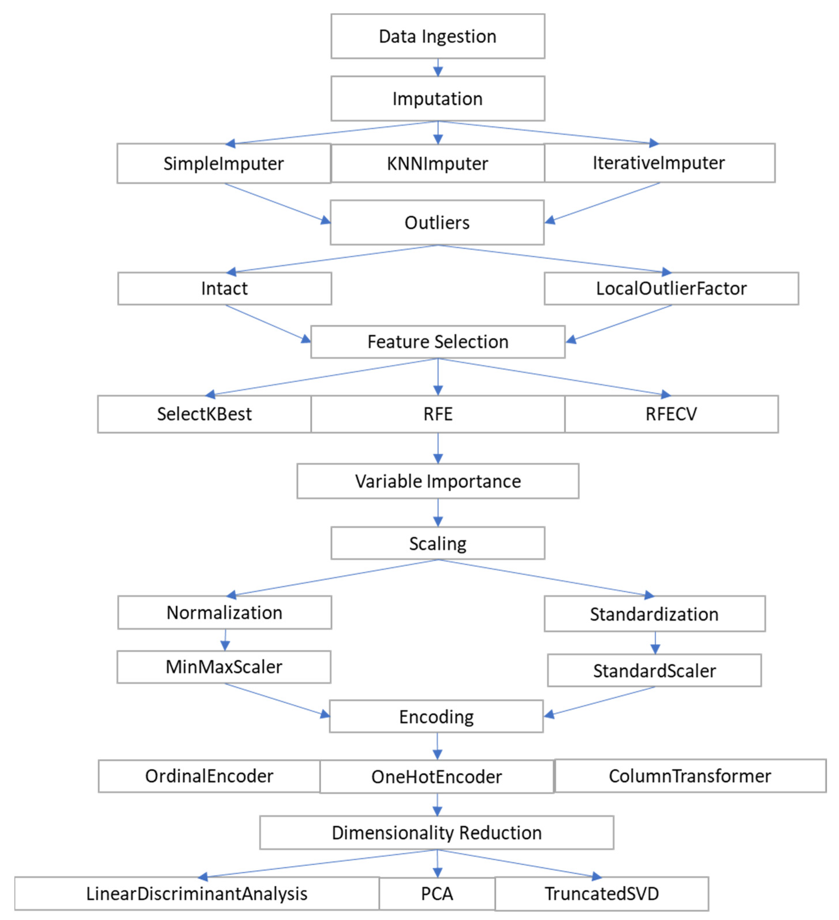
4. Analytics Life Cycle Methodology

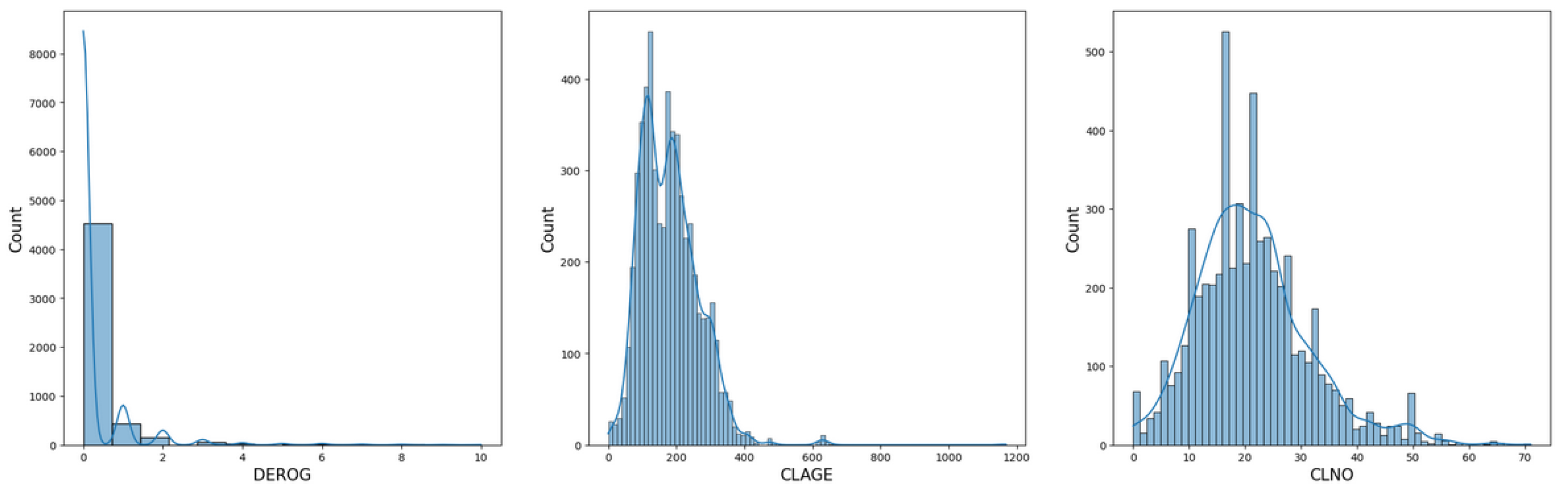
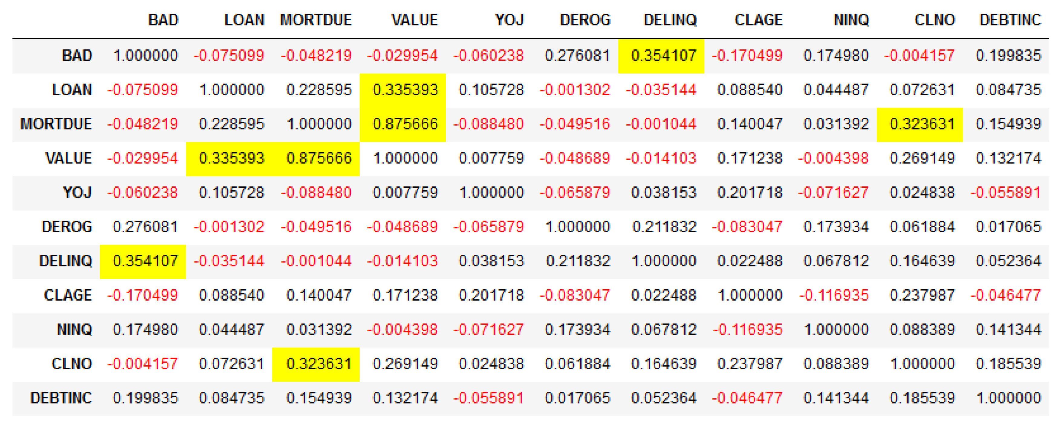
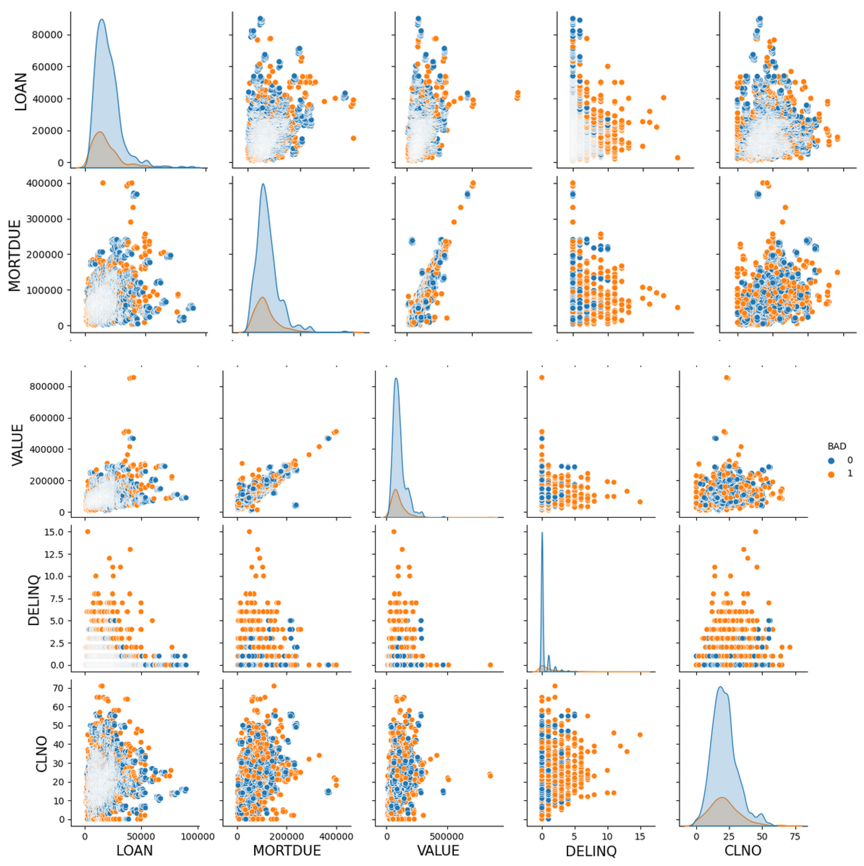
4.1. Exploratory Data Analysis (EDA)

The EDA examines the assumptions, validity, and useability of the dataset, especially for algorithms that are susceptible to the assumptions of Gaussian or near-Gaussian distributions.

There are only a handful of numerical variables to examine, with ‘REASON’ and ‘JOB’ being the categorical variables that will be converted through one-hot-encoding in the data pre-processing step. The distribution for numerical variables (LOAN, DEBTINC, MORTDUE, YOJ, VALUE, DELINQ, DEROG, CLAGE, CLNO) can be summed up in Figure 1.

As seen from Figure 1, the distributions for the numerical variables, in general, followed the normal distribution with some skewing to the right.

A correlation chart is depicted in Figure 2 that highlights any coefficient more than 0.3. None of the negative correlations (highlighted in red) had a significant value. Apart from the MORTDUE and VALUE, which naturally correlated as the higher the value of the loan, the higher the mortgage due, and vice versa. In modelling, highly correlated features can degrade the model performance for some algorithms; however, the tree-base algorithms are largely immune.

A more visual representation of the chart shows the correlation of the variables highlighted in yellow from Figure 2.

From the visual correlation graph in Figure 3, which helped identify the high correlation between the two variables VALUE and MORTDUE, the relationships between the other numerical variables were insignificant. More importantly, it was obvious to see the target variable, BAD, having a skewed (or unbalanced) class, whereby a high percentage (80%) contains 0 and a lower percentage (20%) contains 1. This is reasonable for the loan default scenario as the default rate is usually a much lower figure than the non-default rate. The unbalanced class can pose issues to model performance, which can be circumvented using a weighted approach such as in the case of the classic logistic regression implemented in this paper.

4.2. Data Pre-Processing—Data Preparation

The goal of data pre-processing is to expose the underlying data structure optimally to the respective machine learning algorithms. The data pre-processing step can be considered as the most important step as a careful examination of the underlying data structure will potentially produce results with a higher model accuracy, as various machine learning algorithms are known to be susceptible to the layout of the data. This is true for classic logistic, machine learning algorithms, and Bayesian inference.

This step includes data cleansing, feature engineering, and categorical data encoding for both the input variables and output target. Data cleansing, for example, is carried out by either removing or imputing missing values using various imputation techniques. DEBTINC was imputed using the simple mean impute, DELINQ was set to 0, and JOB was set to ‘Missing’, whilst the rest of the missing values were dropped. This left a total of 4359 (out of the original 5960) observations for sampling. This paper did not require new variables to be derived from the existing variables to better predict the outcome.

Feature pre-processing is a part of the data pre-processing step. To perform feature pre-processing, ordinal variables will undergo either one-hot or label encodings whilst nominal variables can be scaled—either standardised and/or normalised—as the importance of scaling cannot be minimised. Since REASON and JOB are the only two categorical variables, one-hot-encoding was applied to them both. Normalisation is the process to rescale the values of sample data within the range of 0 and 1, whilst standardisation rescales data to have a mean of 0 and standard deviation of 1. In this paper, scaling was applied to classic logistic regression.

Table 2. Formulas for feature pre-processing.

Feature Pre-Processing
Pre-Processing	Formula
Unprocessed	$x^{\prime }=x$
Normalisation	$x^{\prime }=\frac{x-x_{min}}{x_{max}-x_{min}}$
Standardisation	$x=\frac{x-{\mu }_x}{{\sigma }_x}$

shows the formulas for unprocessed, normalization and standardization.

The data processing was made easy using Python’s Scikit-Learn package (Nelli 2018) whereby numerous data cleansing such as imputation, feature selection, scaling (standardization and normalisation), encoding, and dimension reduction techniques can be created as pipelines. In the pipeline, classic logistic regression, SVM, random forest, decision tree, gradient boosting, and extreme boosting will obtain the best possible hyperparameters using GridSearchCV capability.

Furthermore, to ensure the good practice of no data leakage, proper handling of training, testing, and validation datasets is required. Data leakage affects the accuracy of the model as knowledge of the test or validation datasets leaks into the training dataset during the model training phase. In particular, scaling—either standardisation or normalisation—and feature extraction are prone to data leakage. Additionally, since the target variable BAD is an unbalanced class, stratification during the train–test is carried out to ensure both the training and test dataset contain the same ratio.

As a summary, Figure 4 shows the entire end-to-end process flow for the data pre-processing implemented in this paper, specifically using the Python Scikit’s packages. The process depicted below are all the necessary steps taken prior to modelling using classic logistic regression and machine learning methods.

Depending on the classifier involved, for example, XGBoostClassifier automatically performs missing data handling, scaling, and feature selection and dimension reduction.

The goal of the data pre-processing is to produce high quality data that exposes the underlying structure sufficiently. The resulting data can enable various machine learning algorithms to reap the maximum benefit from model accuracy by optimally fitting certain data structures to the respective machine learning algorithms.

5. Modelling and Measurements

5.1. Modelling Classic Logistic Regression, Machine Learning Algorithms Versus Bayesian Inference

During modelling, the selection of appropriate machine learning models of interest will include traditional parametric algorithms and base machine learning, and advanced machine learning techniques are only used as comparisons. The aim was to examine how accurate the Bayesian logistic regression is when put side by side with classic logistic regression, SVM, random forest, decision tree, gradient boosting, and extreme boosting.

During the model construction phase for classic logistic regression and machine learning algorithms, Scikit-Learn’s pipelining was used in conjunction with the model evaluation process described below, which will ensure that the model performance results are captured in a repeatable and valid manner. This following process is repeated by adding one algorithm at a time.

• Evaluate the algorithms:

  ○

  Make a validation dataset using 80:20 ratio for training and testing;

  ○

  Evaluate various algorithms to produce a baseline;

  ○

  Compare various algorithms using various evaluations such as accuracy, precision, recall, f1, and ROC-AUC.

• Improve model accuracy:

  ○

  Tune each model using hyperparameter settings and Scikit-Learn’s GridSearchCV;

  ○

  Include the use of ensemble methods and further turn ensemble methods.

• Select and finalise a model:

  ○

  Choose the best performing model for each algorithm out of the best hyperparameters already known.

Classic modelling follows the standard methodology in machine learning.

5.2. Bayesian Logistic Regression Modelling

Bayesian modelling uses a different approach with the PyMC3-ArviZ (Kumar et al. 2019) package being the primary toolkit used in this paper.

The Bayesian logistic regression model requires the prior distribution to be indicated in each parameter. As subjective as it can be, priors are beliefs that can be included, together with likelihood (data), to produce posterior distribution with parameters within the credible interval (CI). The challenge with prior is that the choice of priors will determine the outcome of the posterior. In other words, two different priors will produce two different posteriors, although with the availability of more data, they will converge to the same distribution.

As calculating the exact posterior of model parameters is intractable, PyMC3 implements the Markov chain Monte Carlo (MCMC) sampling and generalisation to produce the posterior distribution. In other words, the posterior is estimated by drawing repeated samples from the posterior. Since samples from the posterior distribution can be drawn to make inferences, the result itself is a distribution, rather than a point. The beauty of the posterior is that it contains more than just the mode (MAP), but a distribution that contains within certain uncertainty (e.g., 95% high density interval (HDI)) (Turkkan and Pham-Gia 1993) of the true parameters.

There are a total of three Bayesian logistic regressions models implemented with non-informative priors (the goal was to prove that they converged at the end, and they did). Non-informative priors were selected because of the lack of prior knowledge of the parameters. The first two models require a hands-on approach, whilst the third model is fully automated.

• Bayesian Logistic Regression Model 1—assumes a uniform distribution with large enough lower and upper bounds;
• Bayesian Logistic Regression Model 2—assumes a normal distribution;
• Bayesian Logistic Regression Model 3—assumes an automated built-in GLM model from PyMC3.

Model measurements and comparisons between the classic logistic regression and machine learning models use accuracy, precision, recall, F1 score, and ROC-AUC. These measurements work fine with the classification problem we are addressing. Classification measurements (Tharwat 2021) are defined by the following parameters:

• TP (true positive)—actual is true and predicted true;
• TN (true negative)—actual is false and predicted false;
• FP (false positive)—actual is false but predicted true;
• FN (false negative)—actual is true but predicted false.

However, the comparisons between various Bayesian models only used ROC-AUC (Tharwat 2021), which measures the trade-offs in the true positive versus true negative rates. The higher the area under the curve, the better the prediction power of the model.

Table 3. Formulas for feature pre-processing.

Performance Metrics
Accuracy Measurement	Formula
Accuracy (fraction of accurate prediction from the whole sample)	$Accuracy=\frac{\left(TP+TN\right)}{\left(TP+TN+FP+FN\right)}$
Precision (measures correctness in true prediction)	$Precision=\frac{TP}{(TP+FP)}$
Recall/Sensitivity (measures actual observations that are predicted correctly)	$Recall=\frac{TP}{(TP+FN)}$
F1 (Harmonic mean for precision and recall)	$\mathrm{F}1=\frac{2\ast (Precision\ast Recall)}{(Precision+Recall)}=\frac{2TP}{(2TP+FP+FN)}$

illustrate the formulas corresponding to the performance metrics.

6. Results and Comparisons

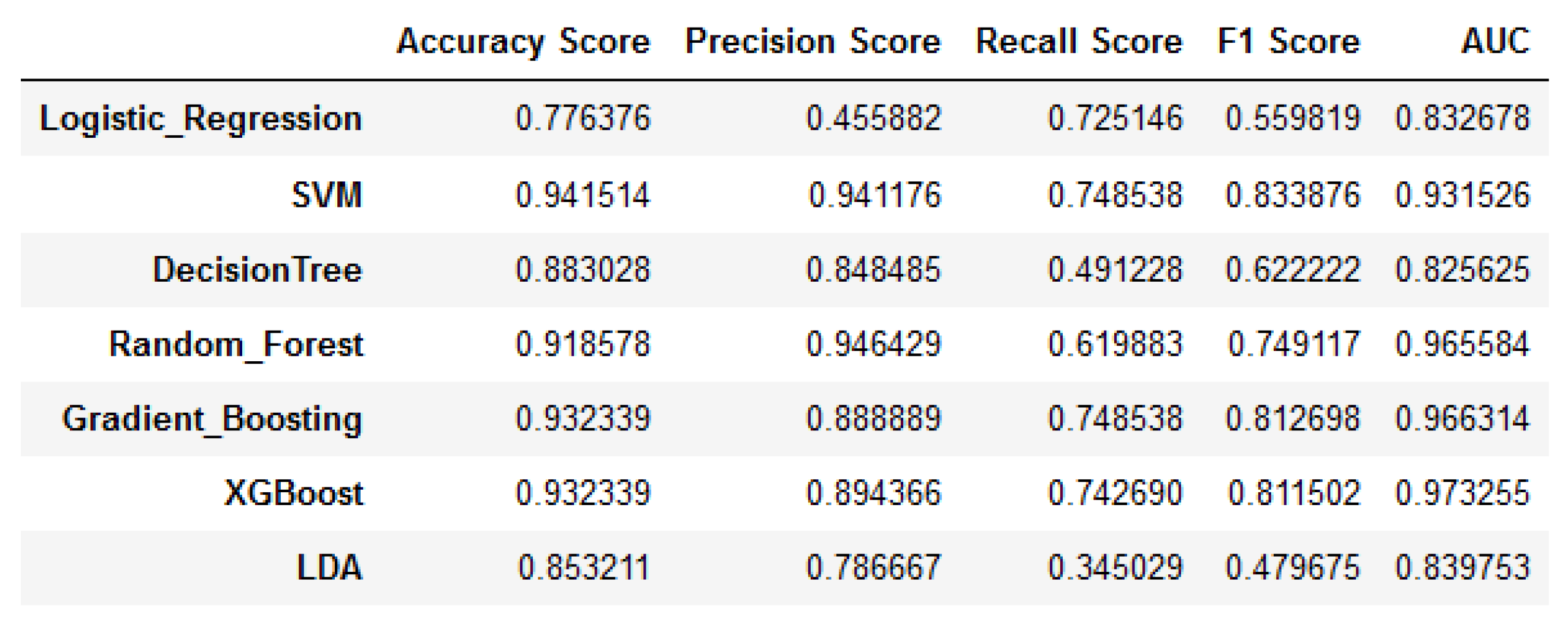
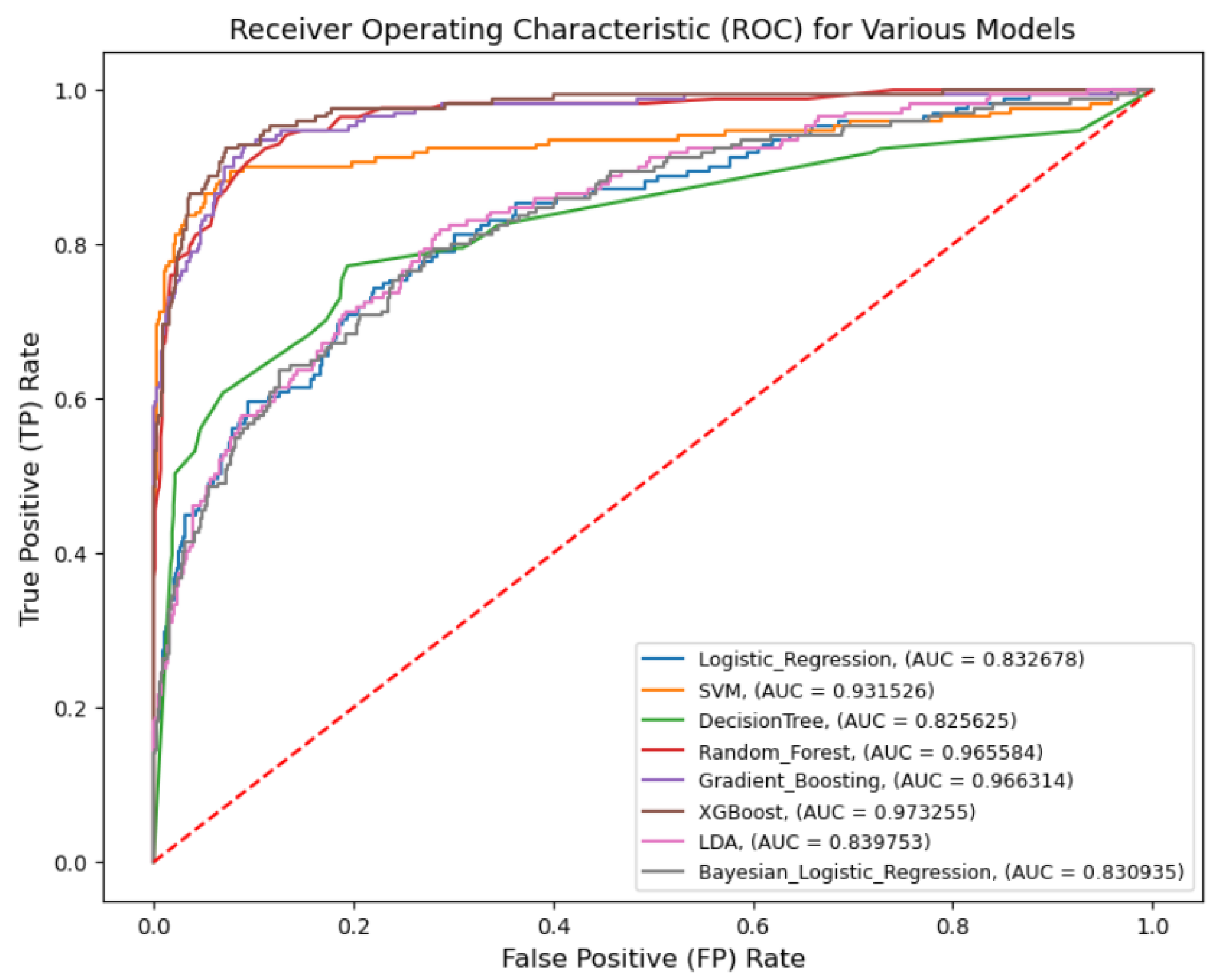
6.1. Classic Logistic Regression, Machine Learning Algorithms, and Bayesian Logistic Regression Model Results and Comparisons

The comparison ran 12 variables to compare the classic logistic regression and the machine learning algorithms with the Bayesian method using the default built-in GLM function. Arviz’s plot trace, as shown in Figure 5, was to assess the convergence of MCMC sampling, and in this case, all MCMC run across three chains converged. The left subplot represents the kernel density estimate (KDE) plot with the tip of the curve being the possible mean. The right subplot represents the individual sampled values.

Whilst the posterior sampling result can be inspected visually, it can be achieved numerically by using Arviz’s summary table, as seen in Figure 6.

For example, using the percentage effect (p_effect), the importance of variables in predicting a bad loan can be made apparent in that the larger (+) or smaller (−) the value, the more of an effect the variable will have on predicting a BAD loan. In this case, with a 1 unit increase in the major derogatory reports (DEROG), the odds of a loan default (BAD = 1) will increase by 125%, whilst with 1 unit increase in the delinquent credit lines, the odds of a loan default will increase by 106%.

Comparable to other classical logistic regression and machine learning approaches, identifying variables of importance is a major part of the exercise during the modelling phase. Variables that do not contribute to the models can be detected and subsequently omitted. For example, in logistic regression, the coefficients, and in random forest/extreme boosting, variables of importance can be generated automatically for comparisons. In PyMC3, the posterior distribution graph helps quantify the uncertainty of variables where the larger the range, the higher the uncertainty. The range of uncertainties for all variables are listed below:

Figure 7, again, apart from the intercept (can be ignored), it is obvious to state that the uncertainty was greatest for REASON, DEROG, and DELINQ. Compared to the rest of the variables, the model clearly indicates that it was less certain regarding these three model parameters.

In the traditional logistic regression, the influence of the variable is reflected in the logit function, and can be used to analyse their importance in predicting an outcome. Similarly, machine learning algorithms implemented today provide a measure to assess the importance of variables. One key advantage of Bayesian is that the ability to interpret and understand the relationships between variables remain intact, although the models can be simple or complex.

Since Bayesian is about sampling the posterior distribution, the Arviz’s plot_posterior provides the mean (or median/mode) to examine the spread of the distribution, with an estimate of the true parameters lying somewhere within. Remember that Bayesian does not necessarily concern the point estimate of model parameter, but uses a posterior distribution to produce a distribution for the potential model parameters to quantify the uncertainty of the true values.

The highest density interval (HDI) indicates the summary of the credible interval (CI) for the posterior distribution. All points resting inside the HDI had a higher credibility, measured as the probability density, than points outside the HDI. This indicates the 95% credible interval, which is the uncertainty of the model from the distribution of the sampled variables.

As shown in Figure 8, for example, the uncertainties for REASON (−0.096–0.34) and JOB (0.038–0.18) were higher than DELINQ (0.62–0.82) and NINQ (0.14–0.24), as the latter two had a narrower range.

The overall performance for classic logistic regression and various machine learning models is summed up in Figure 9. Though various measurements were taken, the most reliable and suitable measure is the ROC-AUC metric listed at the rightmost. In ROC-AUC, the classic logistic regression achieved 0.8327, whilst the highest achievers were XGBoost (0.9733) and gradient boosting (0.9663), with random forest (0.9656) and SVM (0.9315) in the vicinity.

A dedicated ROC-AUC graph for comparison can be seen in Figure 10. The ROC-AUC graph is a more accurate visual representation of model performance with greater area under the curve representing a higher model accuracy. This plot includes the Bayesian built-in GLM method, which when compared with the classic logistic regression did not trail far. For example, classic logistic regression recorded an AUC = 0.8327 and Bayesian logistic regression recorded a similar performance with an AUC = 0.8309 after 2500 samples.

The confusion matrix—using 0.5 as the cut-off point—indicates the following classification accuracy from the use of uniform versus normal priors:

• TP (true positive)—220 versus 221;
• TN (true negative)—2718 versus 2722;
• FP (false positive)—86 versus 82;
• FN (false negative)—463 versus 462.

The confusion matrix report showed similar results from the posterior distributions.

Finally, the effect of the individual variable on the posterior probability could be obtained. This is important as the effect of the individual predictor on the target variable (BAD) was clearly shown.

For example, from Figure 11, the variable JOB had a positive effect on the probability of a loan default. The spread of the lines shows the uncertainty in the estimation of the JOB effect for the model. The bigger the spread of lines, the less certain it is. The variables DEROG and DELINQ had a stronger positive effect (sharper curve) on the probability of a loan default. Again, the spread of lines indicates the uncertainties in the estimate but unlike JOB, both DEROG and DELINQ had higher certainties as the lines were less spread.

The variable, CLAGE, on the other hand, showed a negative effect on the probability of a loan default.

These graphs provide clear indicators as to the effect of the variables in determining the probabilities of loan default. The interpretability is indeed one great advantage for practitioners using Bayesian methods.

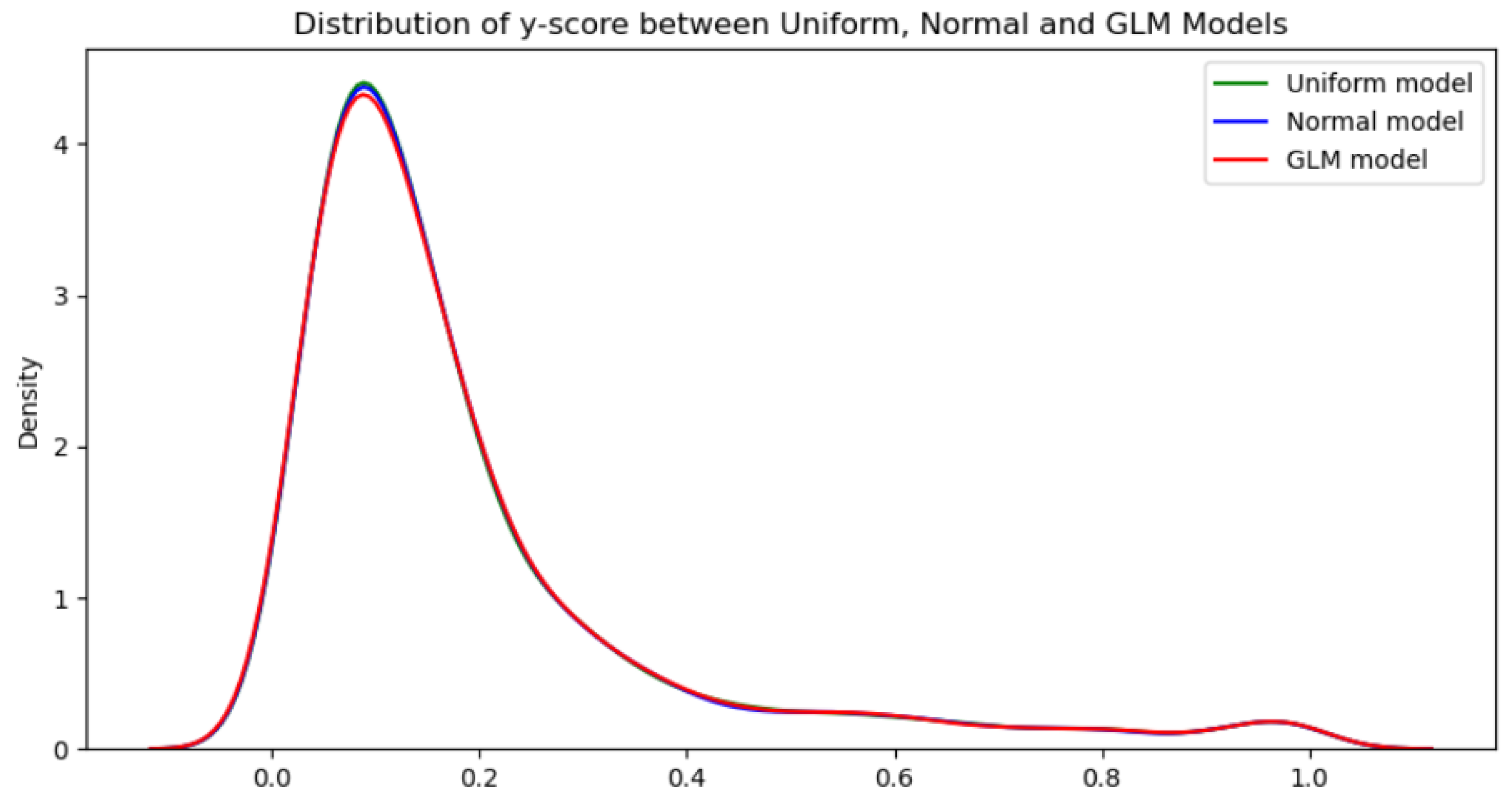
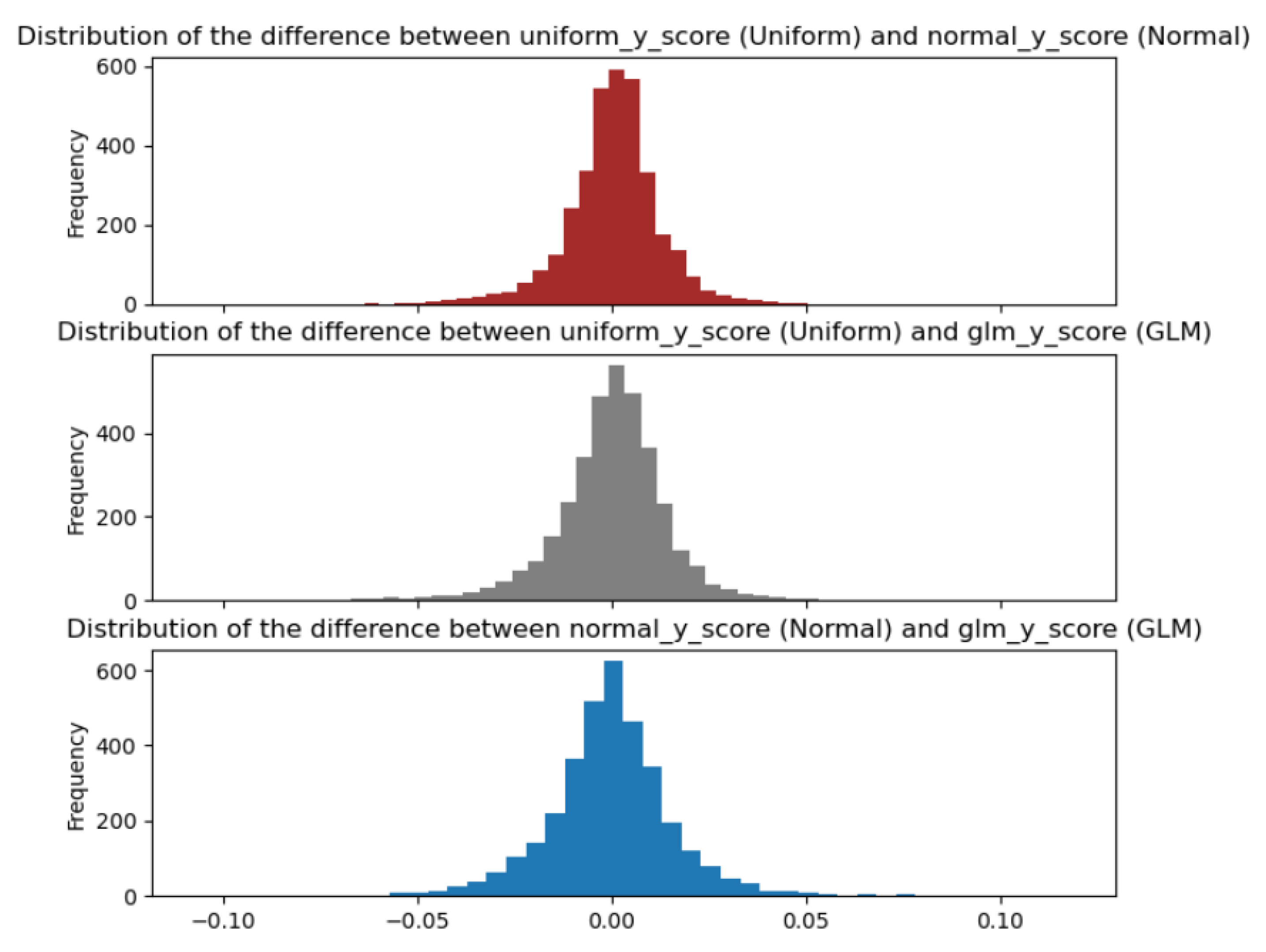
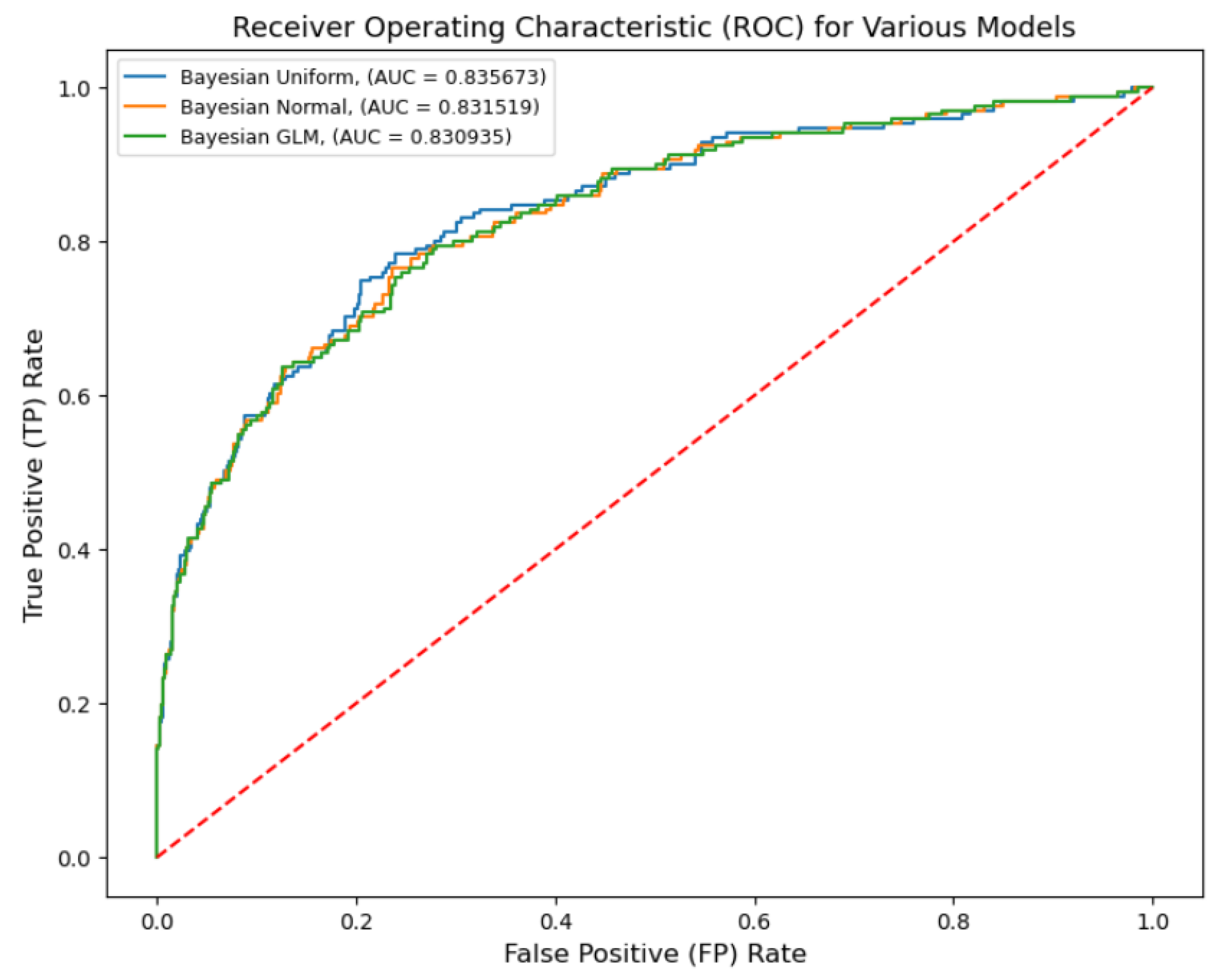
6.2. Bayesian Uniform, Normal, and Built-In GLM Model Results and Comparisons

A comparison was also carried out between the three models based on uniform, normal, and built-in GLM priors. Non-informative priors were selected, and through the MCMC method, the posterior distribution will indicate data relevancy, whether they converge and how quickly they converge. In this comparison, the data were fixed but the priors used were different.

Figure 12 shows that with sufficient samples, all three Bayesian models converged sufficiently quickly to produce diminishing differences in the distributions for the variables, for example, LOAN and DELINQ showed bigger differences in lower samples (2500) than the higher one (9000). For the variable LOAN in the uniform prior model, the converge has happened, but not the ultimate.

Figure 13, on the other hand, shows that the posterior did converge for high samples (further enhancement of the samples was not feasible due to limitations in computational resources). In this scenario, the comparison between 2500 samples versus 90,000 samples further shows that the differences between three models for the variable LOAN became the minimum.

Equally telling is that the mean of the y-score for all three models was close. Note that the difference of y-score between the three models was barely noticeable. From Figure 13, the GLM model yielded the most moderate y-score whilst the other two remained closely knitted with the majority spread centred around 0, followed by a heavy right tail to 1. The spread is in alignment with 80% of HMEQ dataset being non-default (0) and 20% being default loans (1).

The differences in the mean of the predicted y-score drawn from the PyMC3′s posterior predictive sampling barely showed any difference in the distributions. In Figure 14, the first plot shows the difference between uniform and normal priors, the second shows the difference between uniform and GLM, and finally, the third plot shows normal and GLM priors. From the differences in the mean y-score, it can be concluded that the HMEQ dataset converged with all three non-informative priors.

A side-by-side comparison of the coefficients in Figure 15 showed that the coefficients for the Bayesian models (uniform, normal, and GLM) were similar amongst the three. However, the coefficients for the variables REASON and DEROG for the classic logistic regression are far from the Bayesian ones.

The similarities of the ROC-AUC plot for the three Bayesian models can be seen in Figure 16. Here, we can conclude that the data are relevant since the posterior distribution converged to form similar curves: the Bayesian uniform prior model achieved an AUC = 0.8357, the normal had an AUC = 0.8315, and finally, the GLM had an AUC = 0.8309.

Figure 17 shows the ROC-AUC graph for the three Bayesian models. The graph shows the three Bayesian models performance equally well.

7. Conclusions

The advancement of Bayesian in modern world applications has been made possible due to the availability of computational power and the rise in software packages that implement Bayesian methods. For certain classification problems, for example, image analysis, the Bayesian method is the only feasible method to date.

This paper introduced the key concept of Bayesian method in contrast to the frequentist approach. Bayesian is founded on true parameters being a distribution that falls within a probable range called the credible interval (CI).

The key advantage of Bayesian is the incorporation of prior knowledge into the data and model. With a higher sample, a conclusion can be made as the differences between posterior distributions will either diminish or not, which speaks of the data relevancy or irrelevancy to the models. A technique such as MCMC makes the sampling in the Bayesian method possible and exact.

That said, even with the advent of computational power and software availability for Bayesian inference, the adoption of Bayesian amongst the traditional frequentist statisticians is less than ideal due to the subjective nature of the Bayesian method. Bayesian is based on a subjective interpretation of probability with the use of priors, and since priors are subjective, namely, different prior distributions produce different posterior distributions, which render the entire Bayesian interpretation a subjective one, and is therefore considered as the biggest drawback of Bayesian approaches by the frequentists.

Comparisons were made between classic logistic regression, machine learning algorithms, and Bayesian logistic regression (using various non-informative priors), resulting in the following findings:

• From the ROC-AUC measurement, classic logistic regression, various machine learning algorithms, and Bayesian logistic regression achieved a similar performance. Both classic and Bayesian logistic regression might not be the ‘best’ performing models, nonetheless, they are easier to interpret in that the logit can be constructed in both models. In the comparison, eXtreme gradient boosting (XGB) achieved the best score.
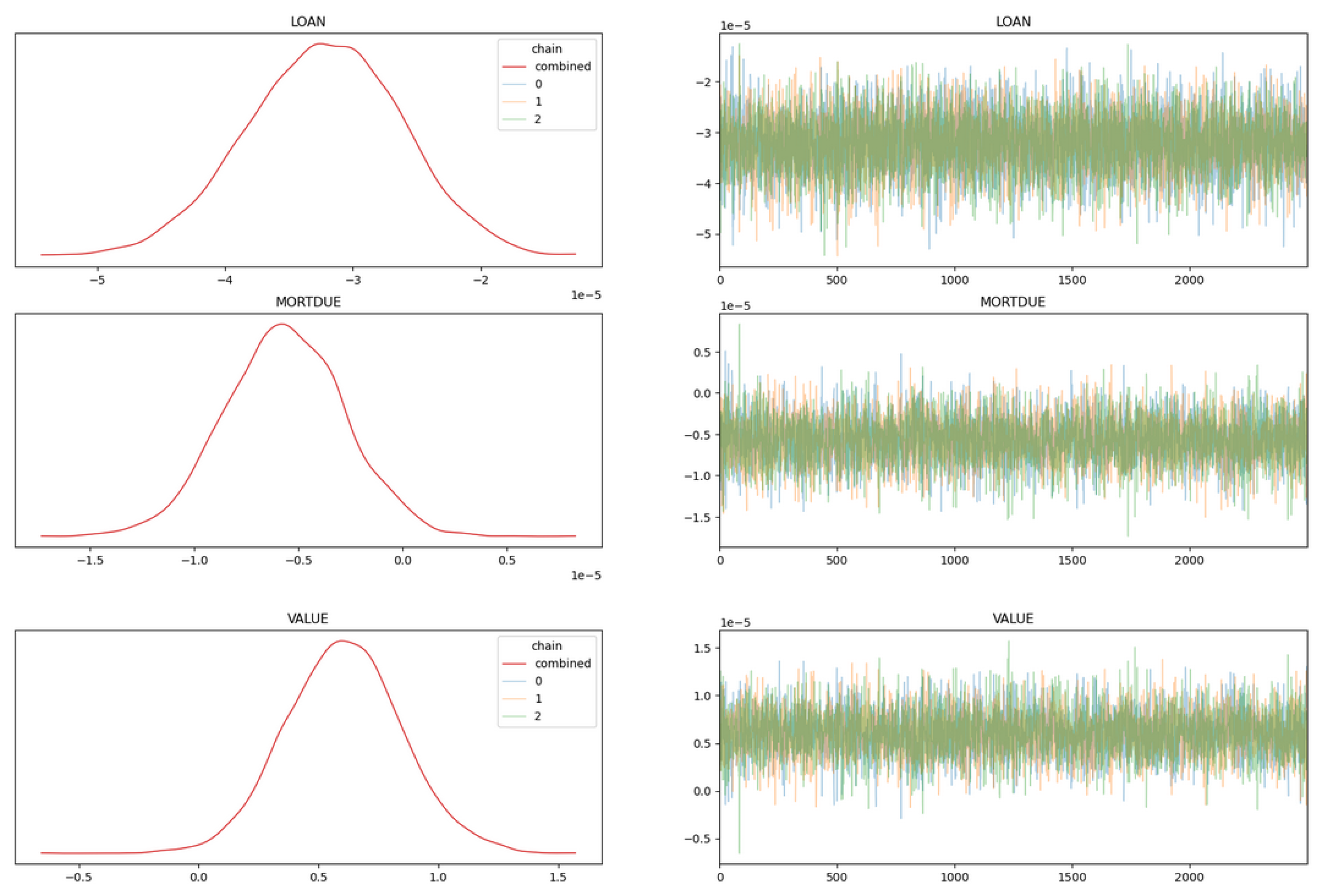
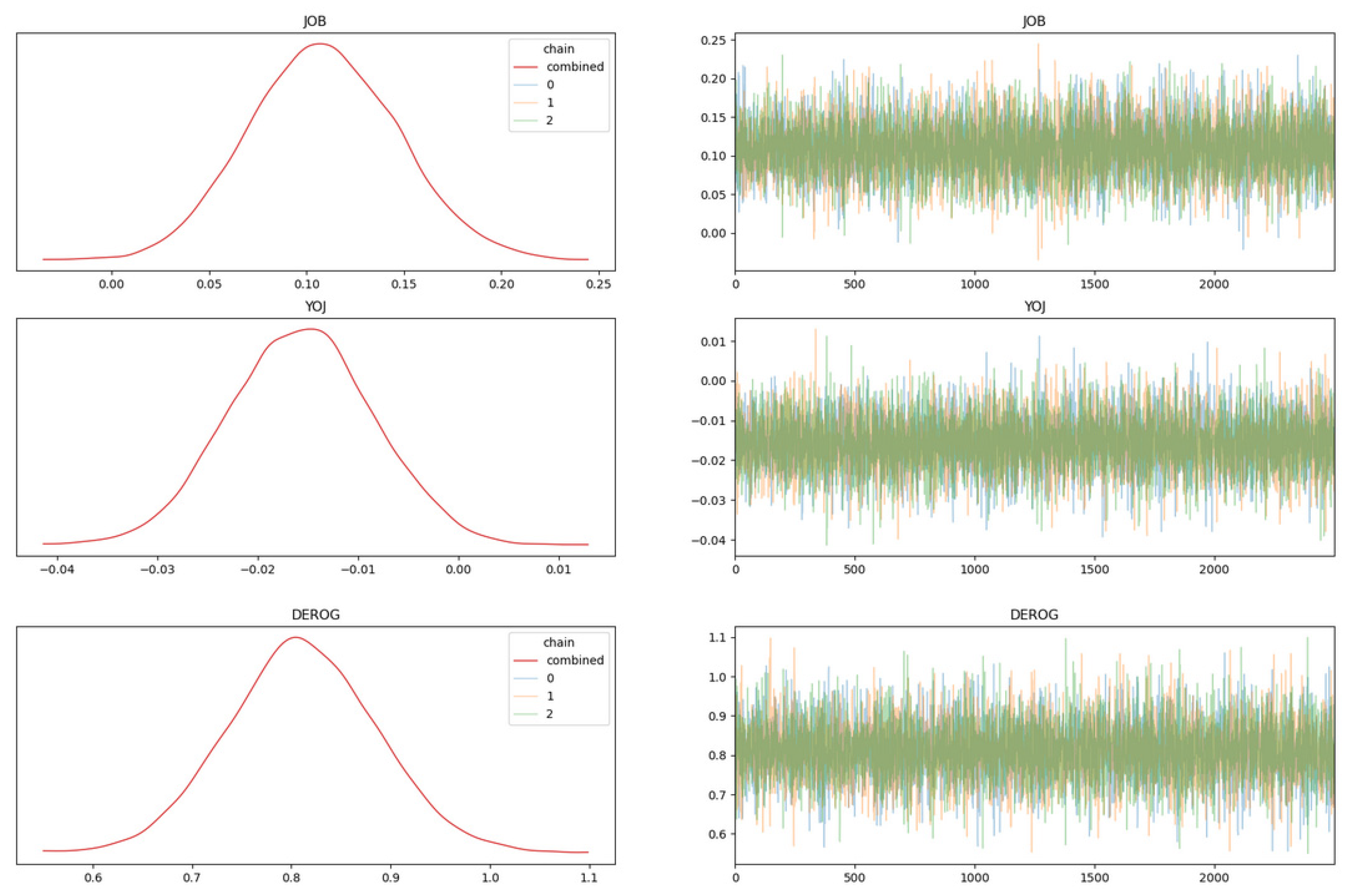
• Uncertainties for variables are clearly displayed and can be quantified for our estimates through various summarisation and graphs provided by Bayesian packages such as PyMC-Arviz. These packages implement the MCMC technique to make posterior distribution sampling tractable.
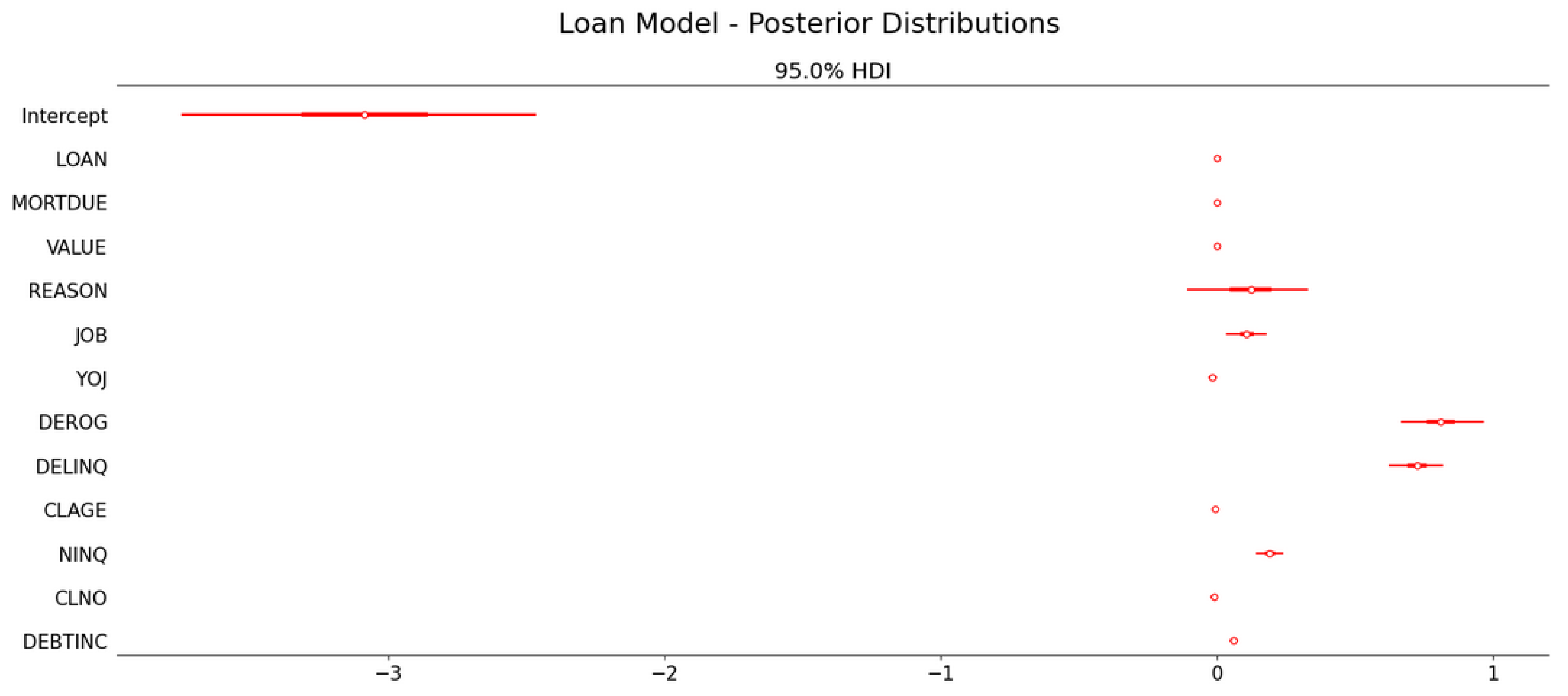
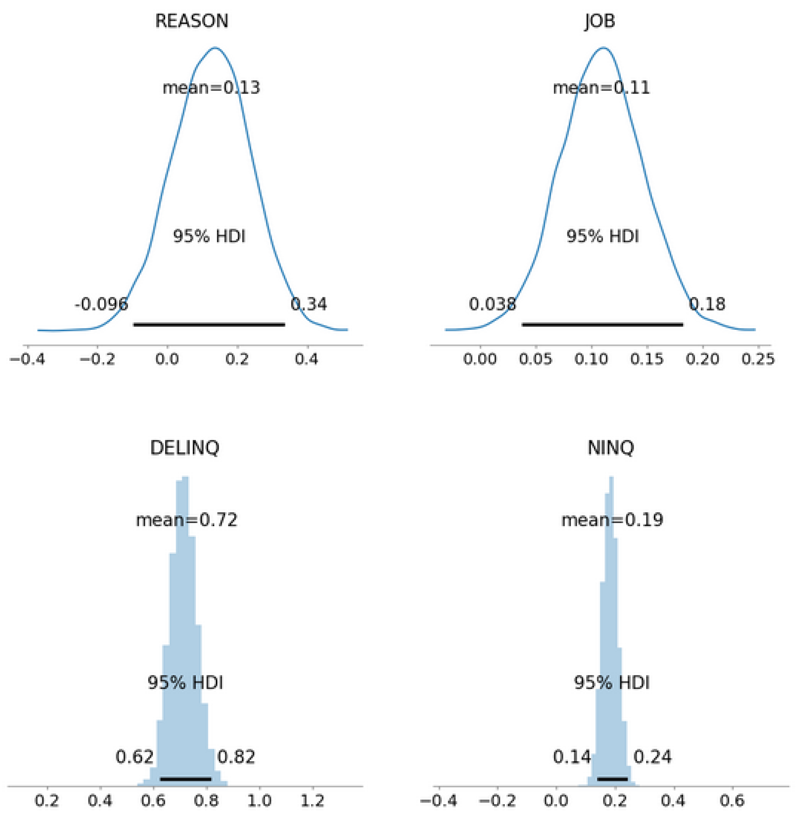
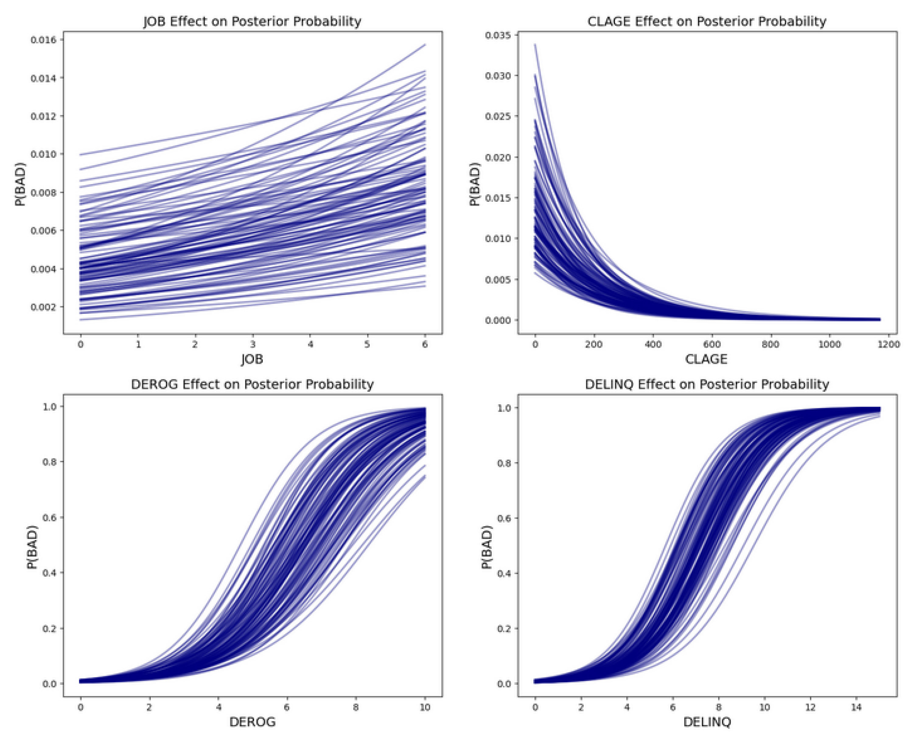
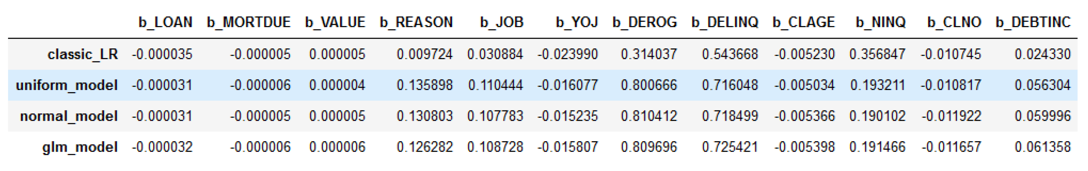
• Bayesian allows models to be interpreted easily and to help discover the relationship between variables and the target variable. For example, the coefficients and percentage effect can be used to assess the importance/influence of the variables toward the models. Additionally, an individual variable effect to the model with a relationship to the target variable can be obtained.
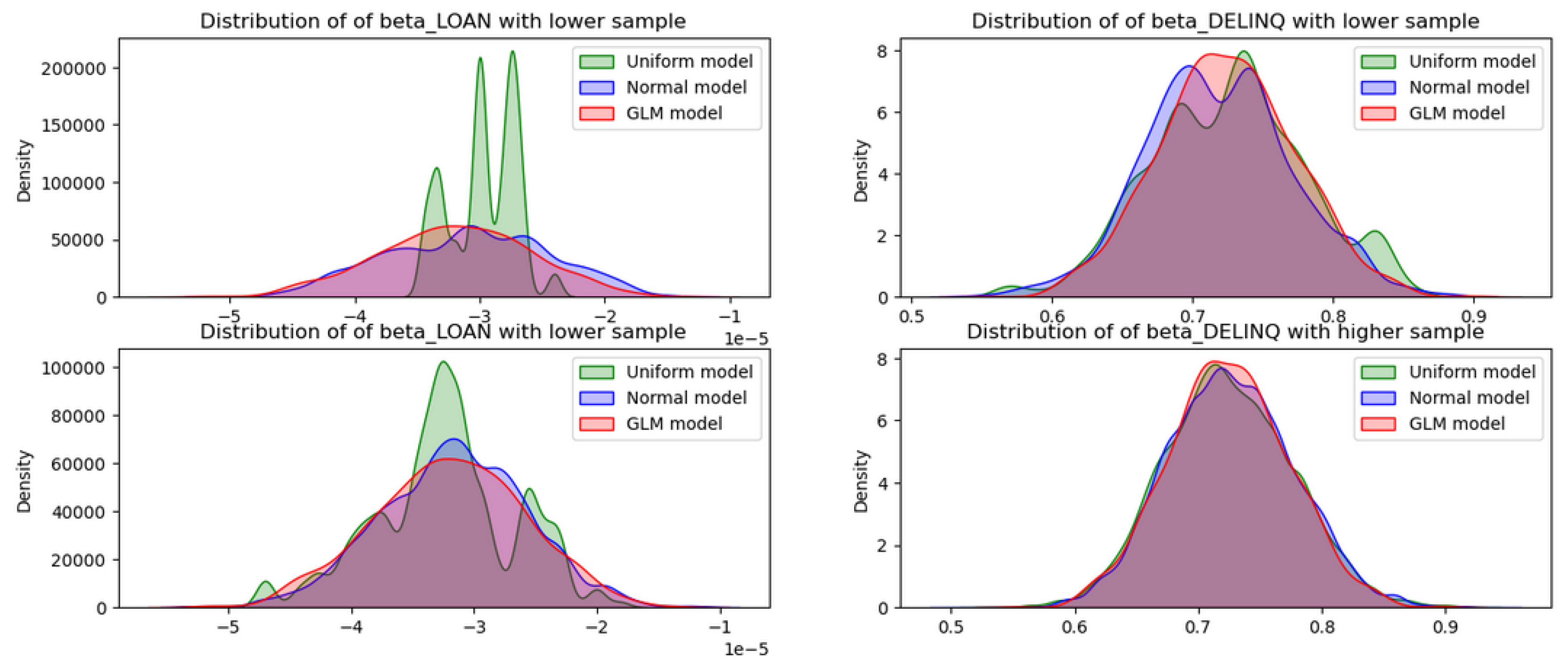
• Subsequently, a test using non-informative priors (uniform, normal, and the built-in GLM methods) for Bayesian created three separate models to prove that they converged relatively quickly. In other words, unless the data provided is highly irrelevant, the models eventually remove the differences in the posterior distribution.

The limitations of this paper were two-fold: the inability to generate higher sampling using the MCMC method due to the computational resource constraint. In this paper, the model generation required enormous resources, even though the dataset was relatively small. This is a tell-tale sign of how a real-life application of Bayesian can be limited by the computational constraint.

Additionally, since including an informative prior is a joint exercise between a Bayesian statistician and a banking domain specialist in the application area (through a process called elicitation) (O’Hagan 1998), this paper took the approach of only using non-informative priors and omitted the inclusion of informative priors.

Further research can be focused on using intuitive probabilistic programming language (PPL) such as PyMC3-Arviz to explore:

• Informative priors for Bayesian logistic regression—this requires solid and proven knowledge to serve as priors;
• Hierarchical models for Bayesian inference—indeed, one huge advantage of using Bayesian is the ability to perform hierarchical modelling. This is an area that has garnered great interest and detailed research in this area will add to the body of knowledge for Bayesian and its modern implementation.

We complete the paper by noting that the methods on statistical distributions and different models (Kobayashi et al. 2022; Kakamu and Nishino 2019; Ohtsuka and Kakamu 2013) could also be examined and compared in our next step of research.

References

- Berg, Sigbjørn Atle, Finn R. Førsund, and Eilev S. Jansen. 1992. Malmquist indices of productivity growth during the deregulation of Norwegian banking, 1980–1989. The Scandinavian Journal of Economics 94: S211–28. [Google Scholar] [CrossRef]
- Berger, Allen N., and Robert DeYoung. 1997. Problem loans and cost efficiency in commercial banks. Journal of Banking & Finance 21: 849–70. [Google Scholar]
- Bernardo, José M., and Adrian F. M. Smith. 2009. Bayesian Theory. Chichester: John Wiley & Sons. [Google Scholar]
- Bijak, Katarzyna, and Lyn C. Thomas. 2015. Modelling LGD for unsecured retail loans using Bayesian methods. Journal of the Operational Research Society 66: 342–52. [Google Scholar] [CrossRef] [Green Version]
- Borison, Adam. 2010. How to manage risk (after risk management has failed). In MIT Sloan Management Review. Brighton: Harvard Business Review, vol. 1. [Google Scholar]
- Congdon, Peter. 2007. Bayesian Statistical Modelling, 2nd ed. Hoboken: John Wiley & Sons. [Google Scholar]
- Fornacon-Wood, Isabella, Hitesh Mistry, Corinne Johnson-Hart, Corinne Faivre-Finn, James P. B. O’Connor, and Gareth J. Price. 2022. Understanding the Differences Between Bayesian and Frequentist Statistics. International Journal of Radiation Oncology Biology Physics 112: 1076–82. [Google Scholar] [CrossRef] [PubMed]
- Gelman, Andrew. 2008. Objections to Bayesian statistics. Bayesian Analysis 3: 445–49. [Google Scholar] [CrossRef]
- Gelman, Andrew, Daniel Lee, and Jiqiang Guo. 2015. Stan: A probabilistic programming language for Bayesian inference and optimization. Journal of Educational and Behavioral Statistics 40: 530–43. [Google Scholar] [CrossRef] [Green Version]
- Geyer, Charles J. 2011. Introduction to Markov Chain Monte Carlo. In Steve Brooks. Handbook of Markov Chain Monte Carl. Edited by Andrew Gelman, Galin Jones and Xiao-Li Meng. Boca Raton: Chapman & Hall/CRC Press. [Google Scholar]
- Kéry, Marc, and Michael Schaub. 2011. Bayesian Population Analysis Using WinBUGS: A Hierarchical Perspective. New York: Academic Press. [Google Scholar]
- Koch, Karl-Rudolf, and Karl-Rudolf Koch. 1990. Bayes’ theorem. Bayesian Inference with Geodetic Applications, 4–8. [Google Scholar] [CrossRef]
- Kumar, Ravin, Colin Carroll, Ari Hartikainen, and Osvaldo Martin. 2019. ArviZ a unified library for exploratory analysis of Bayesian models in Python. Journal of Open Source Software 4: 1143. [Google Scholar] [CrossRef]
- Kobayashi, Genya, Yuta Yamauchi, Kazuhiko Kakamu, Yuki Kawakubo, and Shonosuke Sugasawa. 2022. Bayesian approach to Lorenz curve using time series grouped data. Journal of Business & Economic Statistics 40: 897–912. [Google Scholar]
- Kakamu, Kazuhiko, and Haruhisa Nishino. 2019. Bayesian estimation of beta-type distribution parameters based on grouped data. Computational Economics 53: 625–45. [Google Scholar] [CrossRef] [Green Version]
- Lee, Peter M. 2012. Bayesian Statistics: An Introduction. Hoboken: John Wiley & Sons. [Google Scholar]
- Lunn, David J., Andrew Thomas, Nicky Best, and David Spiegelhalter. 2000. WinBUGS-a Bayesian modelling framework: Concepts, structure, and extensibility. Statistics and Computing 10: 325–37. [Google Scholar] [CrossRef]
- Ma, Zhanyu, and Arne Leijon. 2011. Bayesian estimation of beta mixture models with variational inference. IEEE Transactions on Pattern Analysis and Machine Intelligence 33: 2160–73. [Google Scholar] [PubMed]
- Nelli, Fabio. 2018. Python Data Analytics, with Pandas, NumPy, and Matplotlib. Berkeley: Apress. [Google Scholar]
- O’Hagan, Anthony. 1998. Eliciting expert beliefs in substantial practical applications: [Read before The Royal Statistical Society at ameeting on’Elicitation ‘on Wednesday, April 16th, 1997, the President, Professor AFM Smithin the Chair]. Journal of the Royal Statistical Society: Series D (The Statistician) 47: 21–35. [Google Scholar]
- O’Hagan, Anthony, and Jonathan J. Forster. 2004. Kendall’s Advanced Theory of Statistics, Volume 2B: Bayesian Inference. London: Arnold. [Google Scholar]
- Ohtsuka, Yoshihiro, and Kazuhiko Kakamu. 2013. Space-time model versus VAR model: Forecasting electricity demand in Japan. Journal of Forecasting 32: 75–85. [Google Scholar] [CrossRef]
- Pereyra, Marcelo. 2017. Maximum-a-Posteriori Estimation with Bayesian Confidence Regions. SIAM Journal on Imaging Sciences 10: 285–302. [Google Scholar] [CrossRef] [Green Version]
- Smith, Andrew, and Charles Elkan. 2004. A Bayesian network framework for reject inference. In Paper presented at KDD ’04: Proceedings of the tenth ACM SIGKDD International Conference on Knowledge Discovery and Data Mining, Seattle, WA, USA, August 22–25; pp. 286–95. [Google Scholar]
- Tharwat, Alaa. 2021. Classification assessment methods. Applied Computing and Informatics 17: 168–92. [Google Scholar] [CrossRef]
- Turkkan, Noyan, and T. Pham-Gia. 1993. Computation of the highest posterior density interval in Bayesian analysis. Journal of Statistical Computation and Simulation 44: 243–50. [Google Scholar] [CrossRef]
- Wang, Zheqi, Jonathan Crook, and Galina Andreeva. 2020. Reducing estimation risk using a Bayesian posterior distribution approach: Application to stress testing mortgage loan default. European Journal of Operational Research 287: 725–38. [Google Scholar] [CrossRef]
- Zago, Angelo, and Paola Dongili. 2006. Bad loans and efficiency in Italian banks. Dipartimento di Scienze Economiche-Università di Verona, 1–51. [Google Scholar]