Valuation of Real Options in Crude Oil Production

Abstract

Oil producers are going through a hard period. They have a number of real options at their disposal. This paper addresses the valuation of two of them: the option to delay investment and the option to abandon a producing field. A prerequisite for this is to determine the value of a producing well. For this purpose we draw on a stochastic model of oil price with three risk factors: spot price, long-term price, and spot price volatility. This model is estimated with spot and futures West Texas Intermediate (WTI) oil prices. The numerical estimates of the underlying parameters allow calculate the value of a producing well over a fixed time horizon. We delineate the optimal boundary that separates the investment region from the wait region in the spot price/unit cost space. We similarly draw the boundary governing the optimal exercise of the option to abandon and the one governing the active/inactive production decision when there is no such option.

1. Introduction

Starting in 2008 American oil production has increased. To a great extent this is due to exploitation of diffuse, low-permeability reservoirs previously beyond reach. The successful combination of horizontal drilling and hydraulic fracturing (or fracking) has gone hand in hand with improved geologic knowledge (as new tight plays were added). Needless to say, strong oil prices have played their role in this regard.

A distinctive feature that sets tight oil production apart from that of conventional oil is higher initial depletion rates. In Bakken (North Dakota, Montana, and Saskatchewan in Canada), a well’s daily average production drops by 50% from the first year to the second, and another two thirds from the second to the third year. Consequently, in order to keep production levels, new wells must be developed continually [1]. According to [2], initial decline rates range between 65 and 80 per cent in the first year. This characteristic of quick production applies too to so-called infill wells, which are drilled late in the field’s life to enhance its production by “filling in” areas that have not been fully exploited by earlier wells. Their productive life is very short. Reference [3] focuses on these wells in Texas. In his sample, a typical well’s monthly production falls to one-half of its initial level only seven months into the well’s life; approximately one-half of the well’s total expected production is likely to be exhausted after 18 months. In our analysis below we also mention developed but uncompleted (DUC) wells; here the crucial fracking that breaks open the rock and produces the oil is pending. This broad segment of producers with short operation horizons is the focus of our paper.

Other features of these activities include: lower upfront investment disbursements, lower lifting costs, quicker ramp-up periods, and shorter hedge-ability needs (to mitigate falling prices) [4]. In this regard, Reference [3] suggests that some (though not all) oil firms in his sample use the (New York Mercantile Exchange) NYMEX market to hedge at least a part of their price risk. These characteristics together render this fast production one of the most price-sensitive (elastic) oil production activities globally.

In the summer of 2014 crude oil prices tumbled and have since remained relatively subdued. Stock levels are high across the world, and U.S. crude inventories have reached record volumes. This situation is frequently referred to as a worldwide glut of crude. Other fundamentals (among them sluggish global demand and some (Organization of the Petroleum Exporting Countries) OPEC countries’ deliberate low-price strategy) suggest that more price falls cannot be discarded [5].

Now this paper focuses on two particular (real) options that active fast producers can exercise. The first one is the option to delay extraction. We analyze this option under two different settings depending on whether the oil price change volatility is assumed to be constant or stochastic; interestingly, the former, “myopic” setting can lead to significant undervaluation of the option to defer. Next we assess the option to definitively abandon the well; we calculate its value as a function of oil production cost and the option’s time to maturity. We leave aside some other options that these producers have at their disposal, among them the option to complete a DUC (exploration costs are already sunk) or drilling a new well. Indeed, Reference [4] stresses the importance of paying attention to option-like issues when it comes to raising capital productivity in this extremely capital-intensive industry.

Regarding early works along similar lines, Reference [6] addresses a deferrable opportunity to develop an oil field. The authors also envisage the possibility that oil price can drop low enough to make abandoning the entire project the desirable course of action. They restrict themselves to basic structures so that closed-formed analytical solutions remain mostly within reach. Reference [7] presents some practical case applications, with a focus on the use of real options theory in capital budgeting decisions by an actual oil firm. Reference [8] considers both the option to expand an offshore oil field and that of early decommissioning; in both cases the authors adopt the so-called least squares Monte Carlo approach as developed by Longstaff and Schwartz [9]. On the other hand, Reference [10] considers the use of carbon captured at a coal-fired power station for enhanced oil recovery in mature wells. The timing option is similarly addressed in [11]; it is first considered in isolation and then in interaction with a scale option.

Our paper is organized as follows. After this Introduction, in Section 2 we briefly review the theoretical model for crude oil price (a thorough presentation can be found in Abadie and Chamorro [12]). Our data sample is succinctly described in Section 3 along with the numerical estimates of the underlying parameters. The valuation of a tight-oil well is summarized in Section 4. Then Section 5 considers the option to defer production under the two scenarios mentioned above. As usual, if the option holder is to maximize its value the optimal threshold or “trigger” price must be determined. We calculate these trigger levels for different production costs. The abandonment option is similarly addressed in this section. Here we calculate the option value as a function of the initial oil price and production costs. We further delineate the abandonment/continuation regions in the price/cost space. Last, Section 6 concludes.

2. Stochastic Model for Crude Oil Price

Abadie and Chamorro [12] focus on the prospects for U.S. producers of tight oil. In the absence of reliable cost data they pay special attention to revenues. These in turn crucially depend on the behavior of crude oil price in the future. Hence they propose a stochastic model of oil price with three sources of risk. In their model both the spot price and price change volatility show mean reversion. Instead, the long-term price (that serves as the anchor level for the spot price) follows a random walk.

Specifically, in the risk-neutral world the time-$t$ (spot) crude oil price, $S_t$ is assumed to evolve stochastically according to a mean-reverting process like the Inhomogeneous (or Integrated) geometric Brownian motion (IGBM for short):

$$d{S}_t=\left[k(L_t-S_t)-\lambda S_t\right]dt+{\sigma }_t{S}_{t}d{W}_t^1;$$

(1)

In this equation, $k$ denotes the speed of reversion of $S_t$ towards the long-term equilibrium level in the physical, real world $L_t$. In addition, $\lambda$ stands for the market price of risk. ${\sigma }_t$ is the instantaneous volatility of oil price changes. And $d{W}^1={\epsilon }_t^1\sqrt{dt}$ is the increment to a standard Wiener process where ${\epsilon }_t^1$ has a standard normal distribution. Equation (1) can be equivalently rewritten as:

$$d{S}_t=(k+\lambda )(S_t^{*}-S_t)dt+{\sigma }_t{S}_{t}d{W}_t^1,$$

(2)

where $S_t^{*}\equiv k{L}_t/(k+\lambda )$ denotes the corresponding long-term level under risk neutrality.

We assume that the long-term equilibrium price $S_t^{*}$ follows a geometric Brownian motion with zero mean and constant instantaneous volatility:

$$d{S}_t^{*}=\upsilon S_t^{*}d{W}_t^2.$$

(3)

It is determined by market prices of futures contracts with distant maturities. Besides, the volatility of price changes is mean-reverting too:

$$d{\sigma }_t=\nu ({\sigma }^{*}-{\sigma }_t)dt+\varsigma {\sigma }_{t}d{W}_t^3.$$

(4)

Here ${\sigma }^{*}$ stands for the long-term equilibrium level towards which ${\sigma }_t$ tends to revert over time at speed $\nu$. And $\varsigma$ denotes the instantaneous volatility (assumed constant) of this process. In principle the above stochastic processes can well be cross-correlated so we must account for this:

$$E(d{W}^1,d{W}^2)={\rho }_{1,2}dt;E(d{W}^1,d{W}^3)={\rho }_{1,3}dt;E(d{W}^2,d{W}^3)={\rho }_{2,3}dt.$$

(5)

This model implicitly assumes that crude oil price is not affected by the activity of any single unconventional oil producer. This seems reasonable since this sector’s output represents a small fraction of world output. According to [13], in 2015 world production of unconventional oil was 4.98 million barrels per day, whereas world oil production was 91.67 Mb/d [14]. Certainly the proportion is much higher at the US level, however. Unconventional oil seems to have affected oil prices there (without it, they would be slightly higher). Presumably this would affect also the prices of futures contracts on crude oil. To the extent that, in our empirical application below, we use the prices of futures contracts on WTI, it seems reasonable to assume that futures prices somehow reflect the opinion of market participants about the future impact of unconventional production on oil prices.

3. Sample Data and Numerical Estimates

The Intercontinental Exchange (ICE) is an electronic marketplace where the ICE West Texas Intermediate (WTI) Light Sweet Crude Oil Futures Contract is traded. Prices are quoted in US dollars and cents. Contract maturities reach up to 108 successive months. Our sample period spans almost ten years. Specifically, we have 161,274 daily futures prices from 24 February 2006 to 4 February 2016 An analysis of the potential time-scale relationships between these spot and futures prices can be found in [15].

Readers interested in the details of the econometric analysis are referred to Abadie and Chamorro [12].

Table 1. Parameter estimates as of the last sample day (4 February 2016).

Parameter	Value	Parameter	Value
S0 ($/bbl)	31.36	$\nu$	1.3652
Nearest $F(0,T_1)$ ($/bbl)	31.72	${\sigma }^{*}$	0.3529
k + λ	0.6824	$\varsigma$	0.8638
$S_0^{*}$ ($/bbl)	49.94	${\rho }_{1,2}$	0.5085
${\sigma }_0$	0.8066	${\rho }_{1,3}$	0.0518
$\upsilon$	0.2477	${\rho }_{2,3}$	0.0115

directly shows the numerical estimates of the underlying parameters as of 4 February 2016 (the last day in the sample). The risk-free rate is $r$ = 0.0225, which corresponds to U.S. Treasury 10-year bonds in December 2015. According to the results, only the spot price (with stochastic volatility) and the long-term price display a comparatively sizeable correlation.

4. The Value of a Producing Well

From the above model for oil price, following [16], in the risk-neutral world the time-0 expectation of the spot price at $t$ (or equivalently the price at time 0 of a futures contract for delivery at t) is given by:

$$E_0(S_t)=S_0^{*}+[S_0-S_0^{*}]e^{-(k+\lambda )t}.$$

(6)

On the other hand, let $X_0$ denote the current (t = 0) level of existing reserves (i.e., the reserves at the start of depletion). We assume exponential decline. This is a standard assumption in the literature on oil production [17,18,19]. It results from geological restrictions on the depletion rate (changes in reservoir pressure, water production, etc.). It generally applies independent of the size and shape of the reservoir or the actual drive-mechanism. The reserves available at time $t$ will be:

$$X_t=X_0{e}^{-\eta t},$$

(7)

where $\eta$ stands for the average extraction rate from time 0 to time $t$. The cumulative oil production from time 0 up to time $t$ equals the difference between the initial reserves $X_0$ and those available at time t:

$$Q_t=X_0-X_0{e}^{-\eta t}=X_0(1-e^{-\eta t}).$$

(8)

Hence the instantaneous change in production is given by:

$$d{Q}_t=\eta X_0{e}^{-\eta t}dt\Rightarrow \frac{d{Q}_t}{dt}=\eta X_0{e}^{-\eta t}=\eta X_t.$$

(9)

Therefore the depletion rate in period $t$ is proportional to the remaining reserves at $t$. This implicitly assumes that oil reserves are depleted following a rigid pattern (in particular, independent of oil price), without any flexibility as far as production is concerned. The oil producers sampled in [3] do not seem to change production rates because of oil price changes; see also [20,21].

Now we can compute the time-0 expected cash inflow or revenue accruing to the well over a time interval $dt$ just by multiplying the anticipated oil price times the change in production (i.e., the amount of oil depleted). Hence, summing revenues over all time intervals from time 0 to time $t$ while discounting them at the riskless rate $r$ we can determine the (time-0) expected present value (PV) of the (cumulative) cash inflow to a producing well from now up to time $t$; again, see [12]. For the sake of convenience we compute this expected PV in unit terms, i.e., per barrel of remaining reserves ($X_0$):

$$i(S_0,S_0^{*},t)=\frac{1}{X_0}{\displaystyle {\int }_0^t}[S_0^{*}+(S_0-S_0^{*})e^{-(k+\lambda )t}]\eta X_0{e}^{-(\eta +r)t}dt$$

(10)

This yields:

$$i(S_0,S_0^{*},t)=\frac{\eta S_0^{*}}{\eta +r}[1-e^{-(\eta +r)t}]+\frac{\eta (S_0-S_0^{*})}{k+\lambda +\eta +r}[1-e^{-(k+\lambda +\eta +r)t}].$$

(11)

Note that this unit income does not depend on oil price volatility ${\sigma }_t$.

If we further assume that the cost to producing a barrel of oil is constant $c$, the (unit) net present value (NPV) of the well is given by:

$$npv(S_0,S_0^{*},t,c)=i(S_0,S_0^{*},t)-c.$$

(12)

Admittedly, the assumption of a constant cost is hardly realistic. For one, any producing well will incur fixed annual costs every year in operation; a declining oil production will translate into a rising unit cost. As for variable costs, they can increase too because the proportion of water lifted with the oil grows as depletion continues. It must be similarly admitted, however, that production cost is very difficult to define for several reasons [22]. First, to the extent that it is an important source of firms’ competitiveness, they typically do not publish information about it. In addition, it strongly depends on variables that are specific to each well (location, size, etc.), so it can change markedly from one well to another. Besides, during the depletion phase a number of unexpected expenses can show up (related to the weather, strikes, regulations, …). In sum, usually the production cost can only be determined accurately ex post. Faced with this scenario, any particular ex-ante pattern or proposed behavior for production cost can be considered somewhat ad hoc; we opt instead for the simplest specification and stick to it consistently in all our analyses below.

To use Equation (11) for numerical purposes, in addition to the parameter values in Table 1 we further need to set the depletion rate and the operation horizon. Regarding the former, following [2] we assume $\eta =1.291$; since e^−1.291 = 0.275 this implies that by the end of year 1 the volume of reserves has dropped to 27.5% of the initial level, i.e., in the first year oil production amounts to 72.5% of reserves; see Equation (8). As for the latter, we set $t$ = 10. Under these assumptions we get $npv(S_0,S_0^{*},10,c)=37.07-c$. In words, the net present value (per barrel) will be positive provided $c$ < $37.07/bbl; some of the best wells in the Permian basin now require an oil price about $35 a barrel for an operator to break even [23]. These figures can be interpreted as break-even costs under the NPV criterion (with hedging on the futures market): for any particular pair of prices $(S_0,S_0^{*})$, a unit cost $c$ above $i(S_0,S_0^{*},10)$ will translate into a negative npv.

Table 3. Value of the option to defer investment with and without stochastic volatility.

Cost ($/bbl)	With	Without	% Difference
10	41.00	40.35	−1.6%
15	36.45	35.72	−2.0%
20	31.95	31.10	−2.7%
25	27.65	26.51	−4.1%
30	23.77	22.05	−7.2%
35	20.20	17.87	−11.5%
40	16.91	14.13	−16.4%
45	14.11	10.90	−22.7%
50	11.79	8.22	−30.3%
55	9.74	6.09	−37.5%
60	8.13	4.44	−45.4%

in [12] displays the same calculation but considering a wide range of possible values of spot price and the long-run price. The former turns out to have a relatively stronger impact than the latter. This is consistent with oil reserves that are relatively quick to be put to produce.

5. Numerical Evaluation of Real Options

Management of an oil well has some real options at hand. As usual, maximizing the value of the oil well requires to optimally exercise these options. Among them we can identify: (a) the option to develop an undeveloped oil well; (b) the option to complete a developed but uncompleted well; (c) the option to temporarily shut down a producing well that turns unprofitable (in principle this involves the possibility to restart operations at some time in the future under the “right” conditions); (d) the option to definitely abandon an unprofitable producing well.

Right now, with crude oil prices at relatively low levels, all of these options do not seem equally alluring (recent agreements by OPEC and its allies to cut production notwithstanding). We aim to explore the most relevant ones in this scenario, namely the delay option and the abandonment option. The former clearly refers to the possibility to defer investment up to a pre-specified date in the future (the option maturity); in our case, whenever the investment happens to be undertaken the oil producer will be able to exploit the well over the following 10 years at most (the well’s expected useful lifetime). Indeed, although long-term fundamentals of oil look attractive, [24] reckons that exploration and production firms are taking a wait-and-see approach. The ultimate purpose when assessing the option to defer investment is to determine the optimal time to invest. Following [6], we assume that the decision to defer has no impact on the resource’s depletion pattern (which is fixed). Upon investment, production continues without any interruption; this looks reasonable since most of the available reserves are depleted during the first two years of operation. For simplicity, we also assume that the investment outlay takes place by means of an instantaneous lump-sum expense; this way the owner of an undeveloped reserve receives the developed reserve immediately after that start of development; Reference [25] similarly does not take time-to-build into account. In [26] instead, the facility (an offshore oil platform) takes one year to complete since the initial disbursement; from then on, available reserves can be extracted over 15 years.

The option to delay encompasses several circumstances. For one, the model can be applied to the case in which no capital expenditure has been made and the option holder can turn an undeveloped oil well into a completed one. Similarly, a fraction of the capital expenditures may have been made to develop the well but it is still uncompleted. In both cases full completion requires some (additional) fixed costs to be paid up. Needless to say, the particular level of the unit cost $c$ (including variable cost) would be different in each case, depending on the development costs already incurred. The model could also be applied in principle when the option holder has closed the well early and suddenly wants to re-open it up again. Note, however, that this possibility seems unlikely since most of the reserves are taken from the ground during a short time span and the cost $c$ (including reopening costs) could be pretty high. In sum, these three possibilities fall be more or less within the realm of the option de delay investment. This said, upon investment oil production is assumed to take place without any interruption or abandonment. This seems reasonable because most reserves are taken from the ground during the first two years; we can think of this as selling future production at the time of investment in the futures market. In what follows we assess this option along with the option to abandon the producing well.

For this purpose we use Monte Carlo simulation below. Specifically, we simulate 200,000 random paths. In our discrete-time approximation we adopt time steps of length $\Delta t=1/50$, i.e., almost weekly steps. Since the investment/abandonment horizon is 5 years, each simulation path comprises 250 steps; Reference [26] takes the same 5-year period since the beginning of the offshore oil project until the last date at which the platform can be installed. As further explained in [12], we calculate the corresponding spot prices, long-term prices and volatilities using the following discrete-time scheme:

$$\Delta S_t=(k+\lambda )(S_t^{*}-S_t)\Delta t+{\sigma }_t{S}_t\sqrt{\Delta t}{\epsilon }_t^1,$$

(13)

$$\Delta S_t^{*}=\upsilon S_t^{*}\sqrt{\Delta t}\left[{\rho }_{1,2}{\epsilon }_t^1+{\epsilon }_t^2\sqrt{1-{\rho }_{1,2}^2}\right],$$

(14)

$$\Delta {\sigma }_t=\nu ({\sigma }^{*}-{\sigma }_t)\Delta t+\varsigma {\sigma }_t\sqrt{\Delta t}\left[{\epsilon }_t^1{\rho }_{1,3}+{\epsilon }_t^2\frac{{\rho }_{2,3}-{\rho }_{1,2}{\rho }_{1,3}}{\sqrt{1-{\rho }_{1,2}^2}}+{\epsilon }_t^3\sqrt{1-{\rho }_{1,3}^2-\frac{{({\rho }_{2,3}-{\rho }_{1,3}{\rho }_{1,2})}^2}{1-{\rho }_{1,2}^2}}\right],$$

(15)

where ${\epsilon }_t^1$, ${\epsilon }_t^2$ and ${\epsilon }_t^3$ are independent and identically distributed samples from a univariate N (0, 1) distribution. Equations (13)–(15) follow a general method to obtain correlated random samples ν₁, ν₂ and ν₃:

$${\nu }_1={\epsilon }_t^1,{\nu }_2=\left[{\rho }_{1,2}{\epsilon }_t^1+{\epsilon }_t^2\sqrt{1-{\rho }_{1,2}^2}\right],{\nu }_3=\left[{\epsilon }_t^1{\rho }_{1,3}+{\epsilon }_t^2\frac{{\rho }_{2,3}-{\rho }_{1,2}{\rho }_{1,3}}{\sqrt{1-{\rho }_{1,2}^2}}+{\epsilon }_t^3\sqrt{1-{\rho }_{1,3}^2-\frac{{({\rho }_{2,3}-{\rho }_{1,3}{\rho }_{1,2})}^2}{1-{\rho }_{1,2}^2}}\right]$$

(16)

Correlation coefficients as estimated in Table 1 are used throughout.

5.1. Valuation and Management of the Option to Delay

The time series simulated for $S_t$ and $S_t^{*}$ allow compute at any time the (unit) npv of an investment at that time as the difference between the PV of the (unit) income and the one of the cost (the sum of whatever fixed cost is pending and the variable cost); see Equation (12). We also have the time series of volatility ${\sigma }_t$ along each path. We consider an American-type call option with T = 5 years to maturity. We stick to a producing well with 10 years of expected useful lifetime since its inception. It is possible to invest at any time before the option expiration, so the optimal exercise time is the one that maximizes the option value.

As a previous step to the valuation itself it makes sense to check the goodness of the simulation as such. One way to do it is by comparing the average values (over the 200,000 runs) of the three state variables at the option maturity ($T$ = 5) with their earlier numerical estimates. According to our results, the average spot price is $S_T$ = 49.29 $/bbl; this figure is fairly close to the price 49.33 $/barrel derived from Equation (6) above. Regarding the long-term level, $S_T^{*}$, the average value at $T$ = 5 is 49.95$/bbl, which is also very close to the price 49.94$/bbl estimated before (see Table 1). As for the volatility, the average value of ${\sigma }_T$ is 0.3526; our earlier estimate was 0.3529 (Table 1). These results attest to the overall goodness of fit of our simulation.

Given the values of $npv(S_0,S_0^{*},t,c)$ at any time t (with $t$ ≤ $T$ = 5) along each path, the Least Squares Monte Carlo (LSMC) approach is used [9]. At the option expiration $T$) the value of the investment opportunity $V$, in each path is the maximum of two numbers, namely the value of exercising the option and zero (because the option contract entails a right, not an obligation; should the payoff be negative the holder would simply leave the option expire unexercised):

$$V_T(S_T,S_T^{*})=\max (i(S_T,S_T^{*},T)-c;0)=\max (np{v}_T;0).$$

(17)

The optimal strategy is to exercise the option if it is in-the-money: $np{v}_T\equiv i(S_T,S_T^{*},T)-c>0$.

At earlier times, the same payoff structure remains. A noticeable difference is, of course, that leaving the option unexercised means keeping it alive for one more period, in which case the payoff is no longer zero but the (expected) value of the option next period. The option must be exercised only if exercising immediately is more valuable than the expected cash flows from continuing (i.e., the value of keeping on waiting to invest). This comparison clearly calls for identifying the conditional expected value of continuation in the first place. Since the continuation value depends on expectations about future events, it must be computed by backward induction: one must proceed from some known future value (e.g., at the option maturity) back to the present. Reference [9] uses the cross-sectional information in the simulated paths to identify the conditional expectation function (see also [27]). Specifically, they regress the subsequent realized cash flows from continuation on a set of basis functions of the state variables:

$$E_t\left[e^{-r\Delta t}{V}_{t+\Delta t}(S_{t+\Delta t},S_{t+\Delta t}^{*})\right]\approx a_1+a_2{S}_t+a_3{S}_t^2+a_4{S}_t^{*}+a_5{(S_t^{*})}^2+a_6{\sigma }_t+a_7{\sigma }_t^2+a_8{S}_t{S}_t^{*}+a_9{S}_t{\sigma }_t+a_{10}{S}_t^{*}{\sigma }_t$$

(18)

At any time, considering those paths that are in-the-money and applying ordinary least squares we can get numerical estimates of the coefficients $a_1,a_2,\mathrm{\dots },a_{10}$. Hence it is possible to estimate the “continuation value” at each step from the state variables at that step. Thus before expiration the investment opportunity is worth:

$$V_t(S_t,S_t^{*},{\sigma }_t)=\max \{i(S_t,S_t^{*},t)-c;E_t[e^{-r\Delta t}{V}_{t+\Delta t}(S_{t+\Delta t},S_{t+\Delta t}^{*})|S_t,S_t^{*},{\sigma }_t]\}$$

(19)

Proceeding backwards, at the initial date we get the time-0 option value (together with the optimal exercise pattern all the way through expiration) for that particular random sample:

$$V_0(S_0,S_0^{*},{\sigma }_0)=\max \{i(S_0,S_0^{*},0)-c;E_0[e^{-r\Delta t}{V}_{\Delta t}(S_{\Delta t},S_{\Delta t}^{*})|S_0,S_0^{*},{\sigma }_0]\}$$

(20)

Then we calculate the average option value across all random samples.

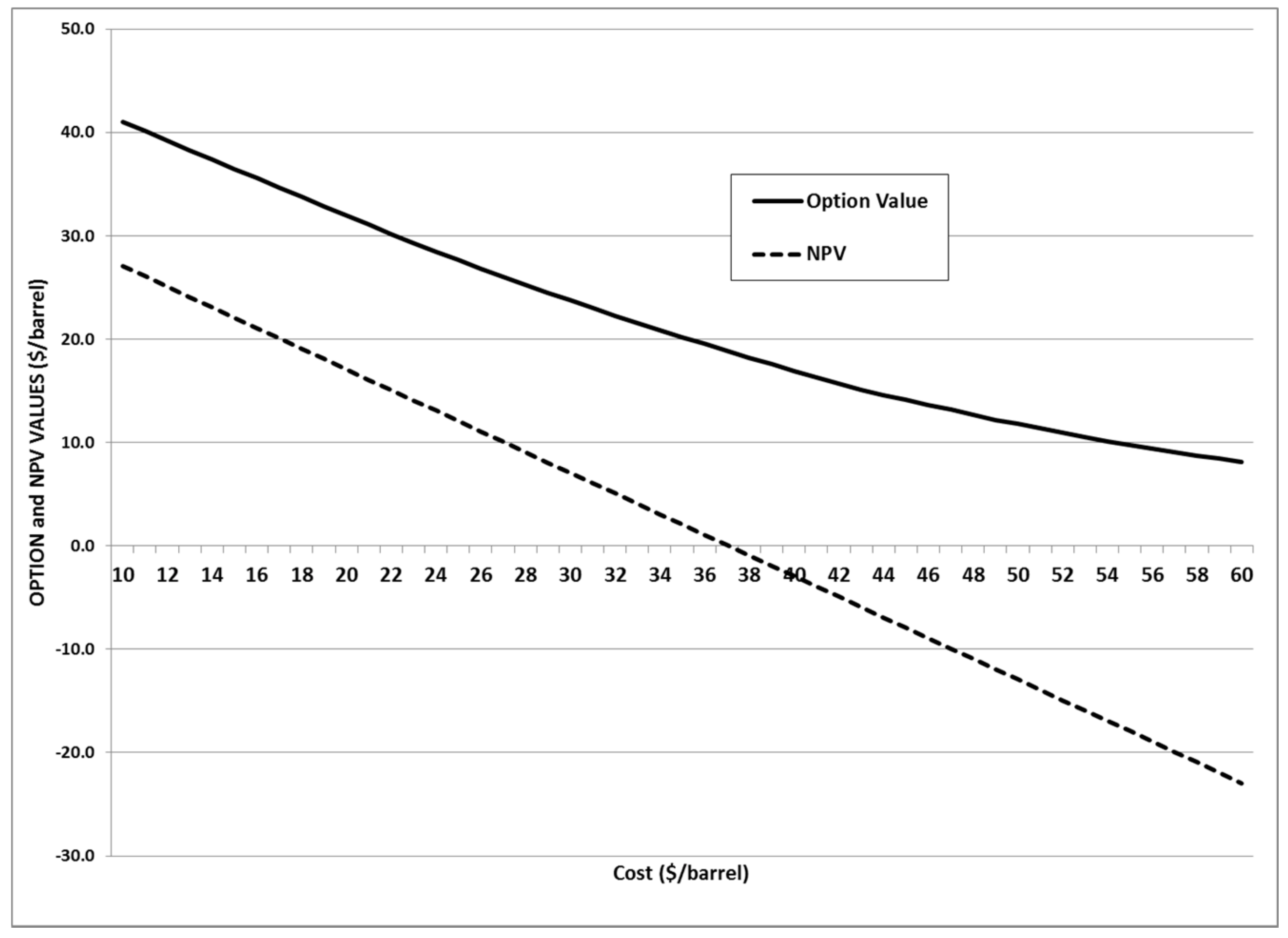
Figure 1 shows the net present value and the option value as decreasing functions of the cost of producing a barrel of oil $c$. The npv, i.e., the value of investing immediately, can be either positive or negative depending on the level of $c$. Instead, the value of the option to invest now or later (if at all) is bounded from below by zero. Besides, it evolves above the npv curve or overlaps it. The vertical distance between them represents the value of the opportunity to wait. Intuition suggests that the distance will increase as the cost $c$ increases; in this case it would be optimal to keep the option alive (and not exercising it). Conversely, there can well be a cost which is so low that the option to wait is worthless and the two curves overlap. In our case, under the initial values of $S$ and $S^{*}$ the option value evolves way above the npv: if it is possible to wait then it is optimal to defer investment.

Figure 2 displays the option value and the net present value in the particular case in which $S_0=S_0^{*}$ = 49.94 $/bbl. Both curves shift upwards but the npv curve undergoes a wider shift than the option value; look for example at the intercept with the horizontal axis. So if there is an option to delay, the optimal decision is to delay investment. Nonetheless the gap between both loci has narrowed significantly: as before, the option holder should not invest yet, but immediate investment is now closer.

As shown in the above figures, at the spot prices considered, if it is possible to wait the optimal strategy is to delay investment. The vertical distance between the two curves remains positive along the costs range considered. This means that there is a value to waiting. As a consequence, the investment should be postponed.

Clearly, when there is no option to wait the decision boils down to whether invest immediately or not. In this case only the npv curve applies and we can follow the standard NPV rule. For example, in the base case (Figure 1) when $c$ = 30 $/bbl we have npv = 7.07 $/bbl, i.e., the trigger cost is 37.07 $/bbl. This value is higher than the current oil price $S_0$ = 31.36 $/bbl (see Table 1); this is mainly caused by the growing pattern (contango) of the crude oil futures market (as of the end of our sample period). Therefore, at the current oil prices under the NPV rule the optimal strategy is not to invest. If current oil price matches the long-term level at 49.94 $/bbl (Figure 2) a cost $c$ = 49.08 makes the npv drop to zero; that number is a bit lower than $S_0^{*}$ = 49.94 owing to the impact of time discounting. As production cost $c$, gets lower the option value and the npv get closer.

In general, for each cost level $c$ there exists a current price $S_0$ (given the oil price in the long run, 49.94 $/bbl) above which it is optimal to exercise the option to invest in a well. For one, Figure 3 displays both the option value curve and the npv for a unit cost $c$ = 30 $/bbl. It will be optimal to invest (thus killing the option to wait) when the two curves start overlapping; this happens at a ‘trigger’ spot price $S_0$ = 75.39 $/bbl. However, when only the NPV applies, with $c$ = 30 we undertake the investment immediately because the PV of the prospective income (37.07 $/bbl) surpasses the cost which results in a positive npv = 37.07 − 30 = 7.07 $/bbl.

In Figure 3 the unit cost is fixed at 30 $/bbl. Now

Table 2. Trigger spot price of the investment option for different unit costs ($/bbl).

Cost	15	20	25	30	35	40
Trigger spot	71.98	72.39	73.72	75.39	78.70	83.00
PV (income)	63.34	63.61	64.47	65.55	67.69	70.47

shows the spot price that triggers investment for a number of different costs (while keeping the long-term price constant). In principle, as the unit cost $c$ increases the spot price required for investing to make sense increases too; this is actually the case here. The PV of future income evolves in the same way.

The former relationship is displayed in Figure 4. Intuitively, when the cost is low and the spot price is high it is optimal to invest (and stop waiting): this is the so-called investment region. Conversely, if the cost is high while the price is low it is better to wait: this is the continuation region. The upward-sloping bold locus represents the pairs (unit cost, spot price) for which the npv and the option value are exactly equal; in this case, management is indifferent between investing and waiting to invest. Out of this boundary one decision is strictly preferred to the other.

5.2. Valuation and Management of the Option to Delay: Myopic Volatility

Now we consider the option to defer without stochastic volatility. Reference [3] observes that failure to respond to changes in oil price volatility by oil producers can entail a substantial cost. Consequently they have a strong financial incentive to assess their options as rationally as possible.

The parameter values are the same as in Table 1, but here we use the long-term equilibrium volatility ${\sigma }^{*}=0.3529$ as crude oil price change volatility (i.e., we leave the parameters ${\sigma }_0$, $\nu$, and $\varsigma$ aside along with the correlations with the spot price and long-term price processes). In this case, with just two (correlated) stochastic processes left we develop a two-dimensional binomial lattice over $T$ = 5 years with 100 steps per year ($\mathsf{\Delta }t$ = 1/100); see [16]. As shown in Figure 5, ignoring the stochastic behavior of volatility consistently underestimates the value of the option de delay.

Since the option to defer is worth less, the reasons for keeping it alive are weaker than before. In terms of Figure 4 this translates into an investment region that grows at the expense of the continuation region. Graphically the optimal boundary (bold line) shifts toward the south east (dashed line); we thank an anonymous referee for raising this point. Further, the underestimation gets more severe as the unit cost increases.

Table 3 sheds more light on this. Thus, undervaluation is relatively less of a problem while unit cost remains below 30 $/bbl. Henceforth the option to delay becomes grossly undervalued.

The ensuing shift in Figure 4 has at least one practical implication. The area that stretches between the two boundaries represents pairs cost-price in which it would be optimal to not invest, yet the firm will do exactly that. This will surely eat into the firm’s profitability and prospects for the longer term. To make matters worse, we observe that the failure aggravates (the gap widens) as the investment cost rises; see also Table 3.

5.3. Valuation and Management of the Option to Abandon

The option to abandon a producing well is conceptually equivalent to an American put option: the option holder can sell the underlying asset or project in exchange for the exercise price at any time up to the option maturity date. We calculate the option value per barrel of remaining oil in the well (at the time when we evaluate the abandonment option). Specifically, a producing oil well involves this real option: upon exercise of the abandonment option its holder gets the difference between the production cost (now saved) and the asset value (now foregone). We set a maximum of $T$ = 5 years for exercising this option. We numerically evaluate it at a particular date, namely the initial time of exploitation, when the well is assumed to have a remaining useful lifetime of 10 years.

At the option expiration ($T$) the value of the option to abandon at the final node on any random path is the maximum of two numbers, namely the value of exercising the option and zero:

$$V_T(S_T,S_T^{*})=\max (c-i_T(S_T,S_T^{*},T);0)=\max (np{v}_T;0)$$

(21)

Obviously the npv refers now to the decision to abandon the well definitively: $np{v}_T\equiv c-i(S_T,S_T^{*},T)$. Another difference with the timing option is that the abandonment option depends on time $T$ because the remaining lifetime of the oil well is 10 – $T$. Further, at time $T$ the PV of the prospective revenues is (see Equation (11)):

$$i(S_T,S_T^{*},T)=\frac{\eta S_T^{*}}{\eta +r}[1-e^{-(\eta +r)(10-T)}]+\frac{\eta (S_0-S_0^{*})}{k+\lambda +\eta +r}[1-e^{-(k+\lambda +\eta +r)(10-T)}]$$

(22)

At earlier times 0 ≤ $t$< $T$ the PV of the cumulative (unit) income becomes:

$$i(S_t,S_t^{*},t)=\frac{\eta S_t^{*}}{\eta +r}[1-e^{-(\eta +r)(10-t)}]+\frac{\eta (S_0-S_0^{*})}{k+\lambda +\eta +r}[1-e^{-(k+\lambda +\eta +r)(10-t)}]$$

(23)

Each particular simulation run gives rise to a particular value of $i(S_T,S_T^{*},T)$. The average simulated unit income across the 200,000 runs at time $t=T$ is 48.50 $/bbl. Time $t=T$ means that the option is exercised at maturity (5 years), and hence the producing well has still 5 years ahead. According to Equation (6), the expected spot price at that date is 49.33 $/bbl. If we now replace $S_0$ for this value in Equation (22) the resulting analytic value is 48.62 $/bbl, which pretty much resembles the simulation average 48.50 $/bbl. So this robustness check seems to perform well.

Similarly to the option to delay, given the values of ${\mathrm{npv}}_{\mathrm{t}}$ along each path the LSMC approach is used. At the option expiration ($T$ ) the value of the abandonment option is determined by Equation (21). At earlier times we follow the same approach as before, Equation (18). Prior to the option maturity the abandonment option is worth the maximum of the exercise value and the continuation value:

$$V_t(S_t,S_t^{*},{\sigma }_t)=\max \{c-i(S_t,S_t^{*},t);E_t[e^{-r\Delta t}{V}_{t+1}(S_{t+1},S_{t+1}^{*})|S_t,S_t^{*},{\sigma }_t]\}$$

(24)

Proceeding backwards, at the initial time $t$ = 0 we get the option value (along with the optimal exercise pattern from then on):

$$V_0(S_0,S_0^{*},{\sigma }_0)=\max \{c-i(S_0,S_0^{*},0);E_0[e^{-r\Delta t}{V}_{\Delta t}(S_{\Delta t},S_{\Delta t}^{*})|S_0,S_0^{*},{\sigma }_0]\}$$

(25)

Assuming an initial spot price $S_0$ = 31.36 $/bbl (see Table 1), a producing oil well with 10 years of expected lifetime, and a saved cost of $c$ = 30 $/bbl, the value of the option to abandon the well is 3.29 $/bbl. Compared to the well’s npv for the same cost (7.07 $/bbl) this means that the abandonment option is worth as much as 45% of the former. Similarly, Reference [26] considers several real options in an offshore oil project, namely learning options, the option to develop, and the option to abandon; the most valuable of them, by and large, is the abandonment option; see also [6,7,28].

Table 4. Value of 5-year option to abandon a 10-year well when $S_0^{*}=$ 49.94 $/bbl.

Spot Price	Production Cost $\mathit{c}$ ($/bbl)
$S_0$	25	30	35	40	45	50	55
20	1.86	3.82	6.82	10.72	15.31	20.28	25.28
22	1.82	3.67	6.48	10.05	14.39	19.08	23.99
24	1.78	3.56	6.19	9.53	13.63	18.16	22.88
26	1.76	3.47	5.98	9.10	13.06	17.40	21.99
28	1.73	3.40	5.80	8.88	12.62	16.77	21.25
30	1.71	3.34	5.66	8.69	12.24	16.28	20.63
32	1.70	3.27	5.53	8.48	11.91	15.86	20.10
34	1.68	3.22	5.42	8.30	11.68	15.51	19.65
36	1.67	3.18	5.33	8.14	11.45	15.21	19.28
38	1.66	3.14	5.25	8.00	11.27	14.93	18.93
40	1.65	3.11	5.17	7.87	11.13	14.69	18.64
42	1.64	3.08	5.10	7.78	10.97	.48	18.39
44	1.63	3.05	5.04	7.68	10.83	14.33	18.15
46	1.62	3.02	4.98	7.59	10.69	14.15	17.93
48	1.62	2.99	4.92	7.50	10.57	14.01	17.74
50	1.61	2.96	4.90	7.42	10.47	13.89	17.58
52	1.61	2.94	4.85	7.34	10.36	13.75	17.43
54	1.60	2.92	4.80	7.27	10.27	13.63	17.27
56	1.60	2.90	4.76	7.21	10.18	13.51	17.13
58	1.59	2.88	4.72	7.15	10.09	13.40	17.01
60	1.59	2.86	4.69	7.09	10.01	13.30	16.87

shows the option value as a function of $S_0$ and $c$. All else equal, if the initial spot price of oil increases the abandonment option is less likely to be exercised and consequently less valuable. Conversely, a rise in the extraction cost renders cessation of operations ever more economically reasonable and the option is worth more.

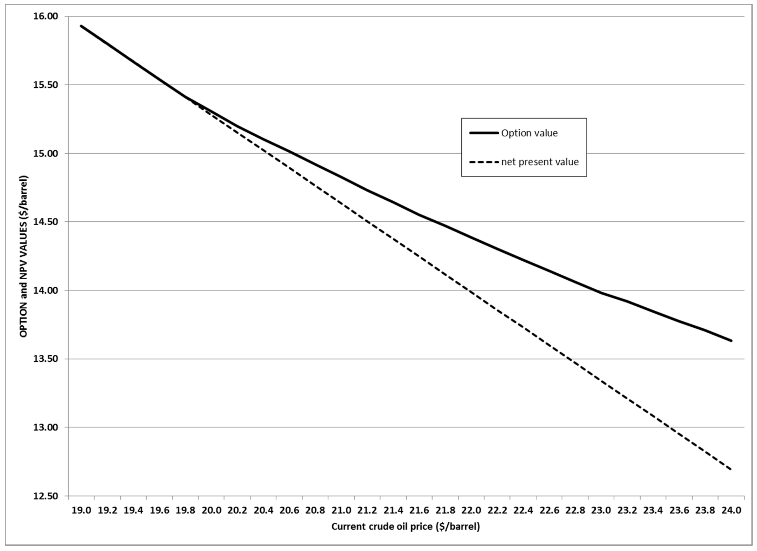
Figure 6 displays the npv and the option value as a function of the current oil price ($S_0$) for a particular cost ($c$ = 45 $/bbl). Moving leftwards both functions overlap for the first time at $S_0$ = 19.81 $/bbl; above this threshold the option value is higher than the npv so it is better to keep it alive (by not exercising) and wait, because oil price can rise more than expected (note that the abandonment option has 5 years to maturity). Instead, below 19.81 $/bbl the two functions overlap, i.e., there is nothing extra to be gained from the option with respect to immediate abandonment. Therefore the optimal strategy is to exercise the option and leave the oil well; this specific trigger price (19.81) depends on the specific cost $c$ saved by leaving. If for whatever reason the firm cannot afford losses and is unable to preserve the option alive then the NPV rule applies. The question here is: given $c$ = 45, at what spot price does the npv switch from positive to negative? In other words, what is the intercept of the npv curve along the horizontal axis? Though not shown in Figure 6 the trigger price is $S_0$ = 43.63 $/bbl. Apart from this, as a general rule the option trigger price converges to the npv trigger price as the option’s time to maturity decreases.

Now Figure 7 draws the optimal boundary between the abandonment region and the continuation region (bold line) in the spot price/unit cost space; along this line the producer is indifferent between remaining in business and quitting. The boundary of the NPV rule is displayed too (dashed line); along this line npv = 0. Starting with the latter, the dashed line divides the space in two parts. On the north-west side $S_0>c$, which suggests that the producing well is making a profit (npv > 0) and should be kept open. Instead, to the south-east $S_0<c$ and the well is making a loss (npv > 0) so closure is optimal. Regarding the option boundary, it obviously applies when it is possible to abandon the well in the future. Since uncertainty can unfold favorably in the future but abandonment is considered an irreversible decision, for any given production cost optimally abandoning the oil well will require a lower oil price than before. This is why this locus evolves below the npv boundary (and is closer to the horizontal axis). We thus have three different regions: (i) the high region, in which the oil well is definitively open (whether or not there is an option to abandon because this is worthless); (ii) the intermediate region, in which the oil well makes a loss but remains open in presence of the abandonment option or is closed otherwise; (iii) the low region, in which the firm is making a loss and there is no point in waiting to abandon, so it is time to definitely close the oil well down.

Last, the value of the option to abandon clearly depends on the option time to expiration. Figure 8 displays this relationship. The abandonment option is more valuable as the saved production cost increases. Nonetheless, whatever the level of $c$, the option is worth less as it approaches maturity: as expiration gets closer there is less room for favorable surprises, so the line jumps downward steadily.

5.4. Exercise of the Option to Defer and the Option to Abandon

The time at which an oil producer should invest for taking oil from the ground, or close down the well definitively, can well be of interest for its future viability; we thank again an anonymous reviewer for bringing this issue to our attention. We address this suggestion for both options. In addition to the base maturity of T = 5 years, below we also consider the case with T = 1. Remember that we run 200,000 simulations.

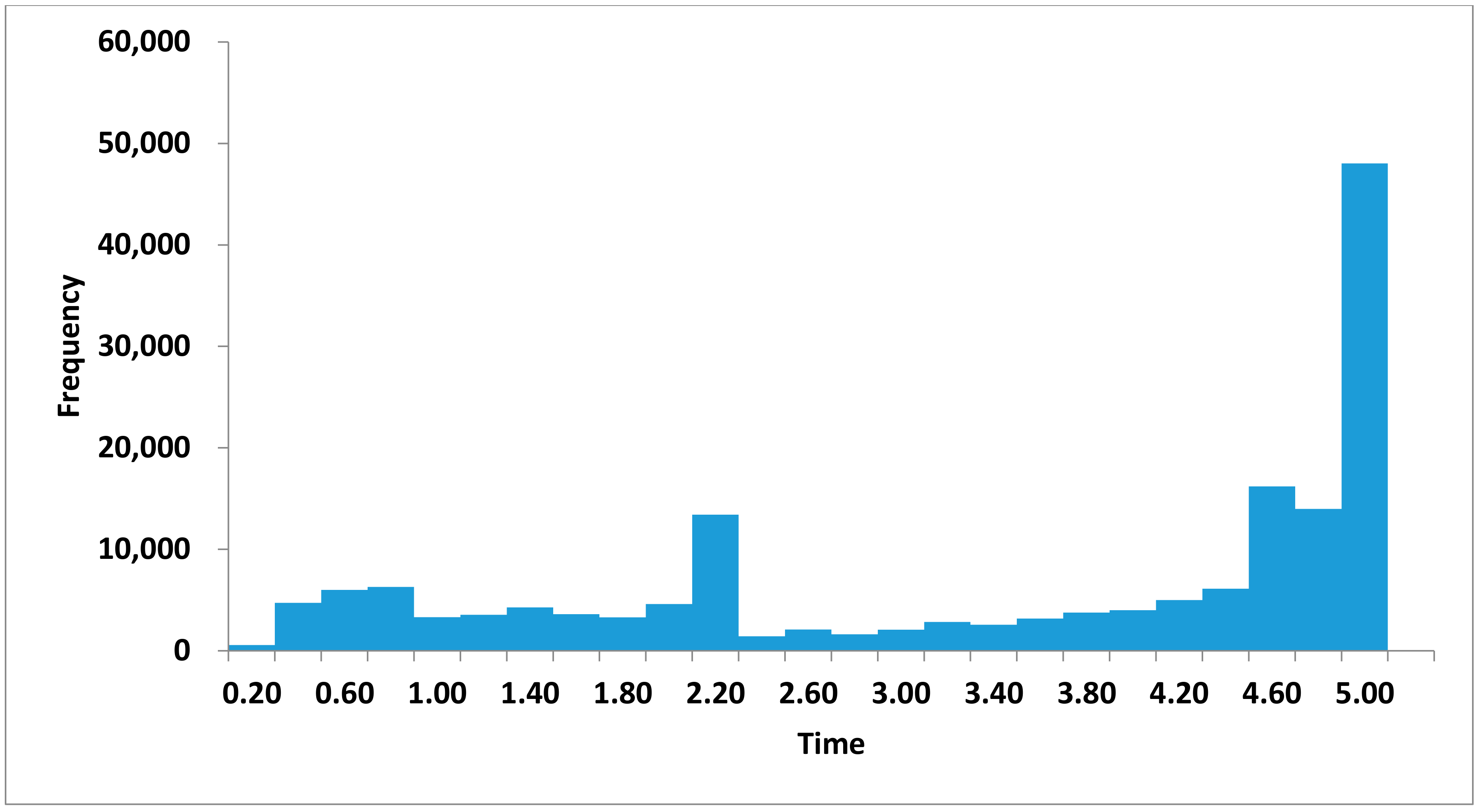
Regarding the option to defer, the results are summarized in

Table 5. Exercise of the option to defer investment.

Maturity	Number	Percentage	Mean	Standard Deviation
T = 1: Without investment	24,843	12.4%	-	-
T = 1: With investment	175,157	87.6%	0.756	0.247
T = 1: Total	200,000	100.0%	-	-
T = 5: Without investment	33,431	16.7%	-	-
T = 5: With investment	166,569	83.3%	3.430	1.617
T = 5: Total	200,000	100.0%	-	-

. Looking at the bottom block (T = 5, base case), we learn that 16.7% of the times there is no investment. In the remaining 83.3% of the cases the average time to invest is 3.43 years, with a standard deviation of 1.61 years.

Figure 9 sheds more light on this issue. Clearly, for the sample period considered, most of the investment cases take place at the very end of the option’s lifetime. This suggests that the incentives for waiting are rather powerful: only when it is no longer possible to wait there seems to be a strong case for investing. A closer look also shows a small peak around the middle of the time to maturity; at this time the value of the option is still important (it is at its half-life) but oil prices (foregone revenues) may be too high for keeping on waiting to invest.

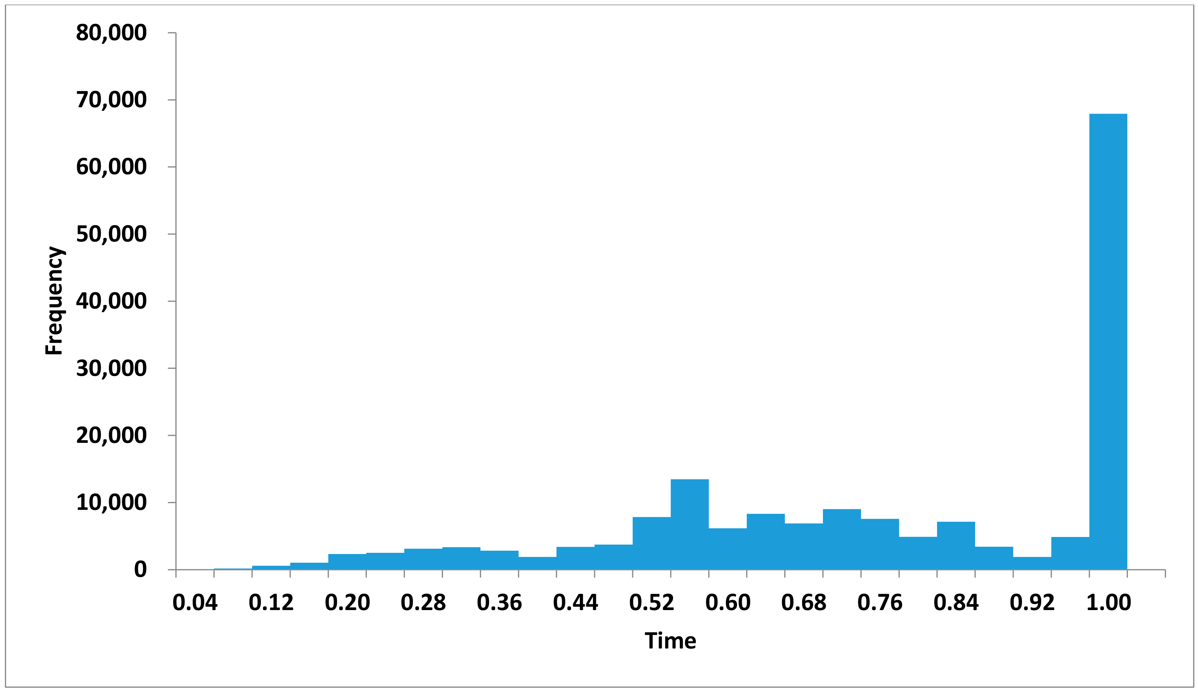
We have undertaken a similar analysis for a much shorter maturity of T= 1 year (top block in Table 5). The fraction of samples with no investment drops to 12.4%. Intuitively, the value of the option to defer is now much lower than before (T = 5), so the overall value of the opportunity to invest gets closer to the npv, the benchmark for a now-or-never investment. This effect shows up as an increase in the number of cases in which the firms invest, from 83.3% (with T = 5) to 87.6% (with T = 1). They nonetheless take their time for investing; the average is 0.75 (out of 1 year) with a standard deviation of 0.24 years. As can be seen in Figure 10, again most of the firms that undertake investment do so at the very end of the option’s lifetime.

Concerning the option to abandon, the results are summarized in

Table 6. Exercise of the option to abandon.

Maturity	Number	Percentage	Mean	Standard Deviation
T = 1: Without abandonment	148,462	74.2%	-	-
T = 1: With abandonment	51,538	25.8%	0.583	0.295
T = 1: Total	200,000	100.0%	-	-
T = 5: Without abandonment	108,980	54.5%	-	-
T = 5: With abandonment	91,020	45.5%	2.732	1.749
T = 5: Total	200,000	100.0%	-	-

. As shown in the lower block (T = 5, base case), 54.5% of the times there is no abandonment. When the firm exercises the option (in 45.5% of the random samples) the average time to do so is 2.73 years, with a standard deviation of 1.74 years. The two proportions are close to each other; this suggests that the decision to abandon looks to some extent like a matter or chance (say, flipping a coin) with a small advantage in favor of continuing business.

Figure 11 displays the frequency distribution. In this case, for the sample period considered, abandonments tend to concentrate on the tails: they take place either close to the beginning or close to the end of the option time to maturity. They also spread more or less equally on both tails, with a small peak in the middle. This again resembles a matter of chance. Maybe the spot price happens to start from a low level but, since volatility increases with time and maturity is still far in the future, it makes sense to wait and see (instead of abandoning early). Yet if the circumstances do not improve enough by mid course then it is time to stop waiting and definitively abandon business (the small central peak). Conversely, if the spot price happens to start from a high level then it is profitable to remain in business; the situation can well turn sour (volatility is there after all), but there is ample room for maneuver (the option maturity is still very distant). In short, it makes sense to keep operations for a while. If, in the end, the prospects justify it, it is time to quit.

We have developed a similar analysis for a maturity of just T = 1 year (upper block in Table 6). The fraction of samples with no abandonment jumps up to 74.2%. As the time to maturity shortens dramatically the value of the option to abandon is much lower than before (T = 5), so the overall value of the opportunity to invest gets closer to the npv (so the npv-rule applies). This effect shows up as a decrease in the number of cases in which the firm closes down permanently, from 45.5% (with T = 5) to 25.8% (with T = 1). They take some time for abandoning; the average is 0.58 (out of 1 year) with a standard deviation of 0.29 years. As shown in Figure 12, many of them only give up their business in the very end (note that abandonment is irreversible).

6. Conclusions

Right now oil producers with short operation horizons (e.g., tight oil) are going through a hard period. Until recently, high returns from high oil prices combined with falling production costs and short-term production cycles. This combination attracted a lot of lenders and cheap credit [5]. Nonetheless, global oil prices have plummeted since the second half of 2014 (with a few upswings of late). Capital expenditure has fallen consequently. Many companies are struggling to service their debts. In addition to solvency issues, liquidity has become another source of concern.

These producers have a number of real options at their disposal. This paper addresses the valuation of two of them, namely the option to delay investment and the option to abandon a producing well; they look especially important under the current circumstances. The value of these options strongly depends on the future behavior of crude oil price. We adopt the particular three-factor stochastic model for the spot price introduced in Abadie and Chamorro [12]. The model allows for mean reversion toward a stochastic long-term level; the price change volatility is similarly assumed to be stochastic and mean reverting (these characteristics apply too to other commodity prices, so the model could in principle be used beyond oil projects). They estimate their model with daily prices of the ICE WTI Light Sweet Crude Oil Futures Contract which is traded on the Intercontinental Exchange (ICE). Hence they calculate the present value (PV) of the prospective revenues from a producing well (in unit terms, i.e., per barrel of reserves). This (unit) gross value can then be compared with the PV of the (unit) costs to be faced in the future. Depending on whether the resulting (unit) net present value is positive or negative oil producers would make a profit or a loss. According to their estimates, the PV of the revenues to be collected over a ten-year period amounts to $37.07/bbl in the base case. Thus, as long as the cost of producing a barrel of oil is lower than $37.07 keeping a producing well in operation will make sense.

Here we value both the option to delay investment and to abandon a producing well by Monte Carlo simulation. Specifically we simulate 200,000 random paths in each case. Regarding the former, the investment horizon is 5 years. Upon completion in this period the well is assumed to have an expected lifetime of 10 years. From the simulated discrete-time paths of the three risk factors in the model it is possible to compute the net present value of investing at any time over those paths. Nonetheless, since the option is of American type, the optimal exercise time must be determined. This calls for calculating the continuation value at any time prior to the option expiration. At this point we adopt the least squares Monte Carlo approach. This way we derive the option value. It is then compared with the net present value. According to or results, if there is an opportunity to delay investment then it is optimal to wait. And if that possibility is not available then it is optimal not to invest. Note that the simulated paths start from the last day in our sample (4 February 2016) at which time crude oil prices were relatively subdued. We also delineate the boundary in the spot price/unit cost space that separates the investment region from the wait region. On the other hand, if the volatility of oil price changes is assumed constant (as opposed to stochastic) the option to defer investment gets undervalued, so much so at higher costs. In this case, oil producers might be lured into investing while the optimal decision would be to restrain themselves from doing so. For the sample period considered, most of the investment cases take place at the very end of the option’s lifetime, which suggests that the incentives for waiting are rather powerful.

Concerning the abandonment option, we consider a producing well with 10 years ahead in principle, but which can be abandoned at any time within a maximum of 5 years. Unlike the option to delay, the exercise date of this option impacts the expected lifetime of the well: if the abandonment option is exercised at time $T$ the oil producer forgoes 10-$T$ years of operation. As before, determining the optimal exercise time and the value of the option rest on the use of least squares Monte Carlo simulation. We calculate the value of this option for different combinations of the spot price (now foregone) and the production cost (now saved). Thus, if the spot price is 31.36 $/bbl (as in the base case) and it takes $30 to take a barrel from the ground the option is worth $3.29, or about 45% of the well’s npv for the same cost (7.07 $/bbl). Similarly, assuming a production cost of 45 $/bbl the npv and the option value overlap at a spot price of 19.81 $/bbl and lower; above this threshold the latter is higher so it is better to remain in operation (thus keeping the abandonment option alive). As expected, higher oil prices decrease the value of the abandonment option while higher production costs make it more valuable. We further draw the boundary governing the exercise of the option to abandon and the one governing production decision when there is no such option. These two boundaries delineate three different regions in the spot price/unit cost space. We also show how the value of the option changes in this space as its time to maturity decreases. For the sample period considered, abandonments tend to concentrate -more or less equally- on both tails: they take place either close to the beginning or close to the end of the option time to maturity.