6.1. Study Parameters
This paper uses the IEEE30 node standard test system for power systems. The example system is shown in
Figure 3. The cogeneration unit replaces the 1st and 2nd units in the original system, respectively; the wind farm grid connection node is 16. The relevant parameters of the thermal power unit are shown in
Table 1, and the cogeneration unit is shown in
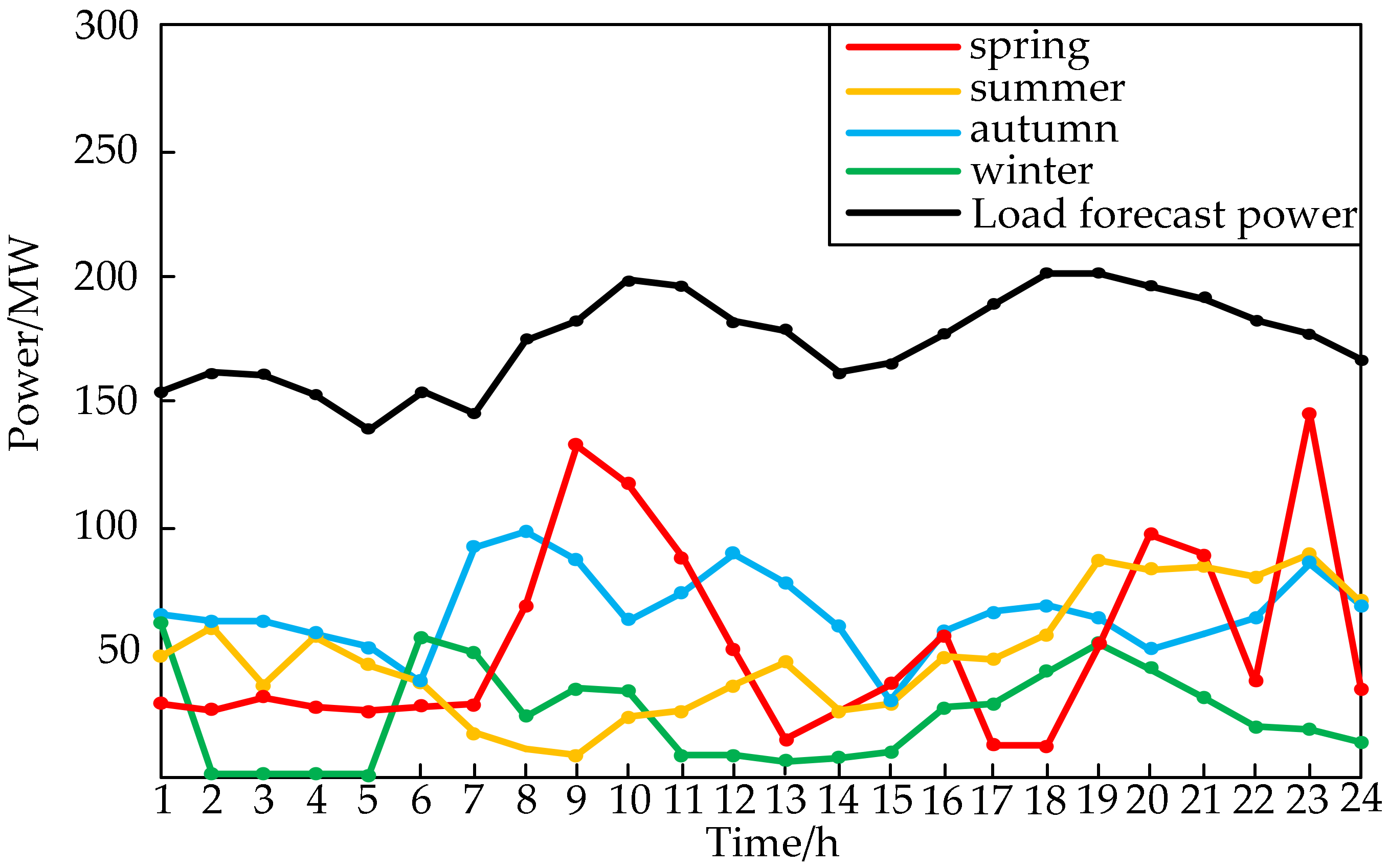
Table 2. In this paper, the wind power consumption is studied according to the wind power field data measured in a certain area. In order to increase the universality of the scheduling process, this paper selects four representative days of spring, summer, autumn, and winter in a year for analysis, the characteristics of four seasons are shown in
Table 3. The scheduling day is divided into 24 scheduling periods for research. Curve of actual measurement of wind power output and predictive power of load are as shown in
Figure 4. The parameter settings in the optimization scheduling process are as follows,
DS,
DN, and
DO are 0.95 kg, 0.95 kg, and 16.7 kg, respectively;
JS,
JN, and J
O are
$0.0893,
$0.0893,
$0.0893, respectively;
fS,
fN, and
fO are 8.5 kg, 7.4 kg, and 16.7 kg, respectively;
J1 is 74.448
$/t; the rotational spare cost coefficient
kr is 34.39
$/MW; the load prediction error
kl is 5%; and the forecast error
kjw of wind farm
i is 15%.
To compare the effects on wind power consumption after the addition of electric boilers, cogeneration units, and green certificate transaction costs, the examples are simulated in the following three ways, as shown in
Table 4.
6.2. Comparative Analysis of Different Scheduling Modes
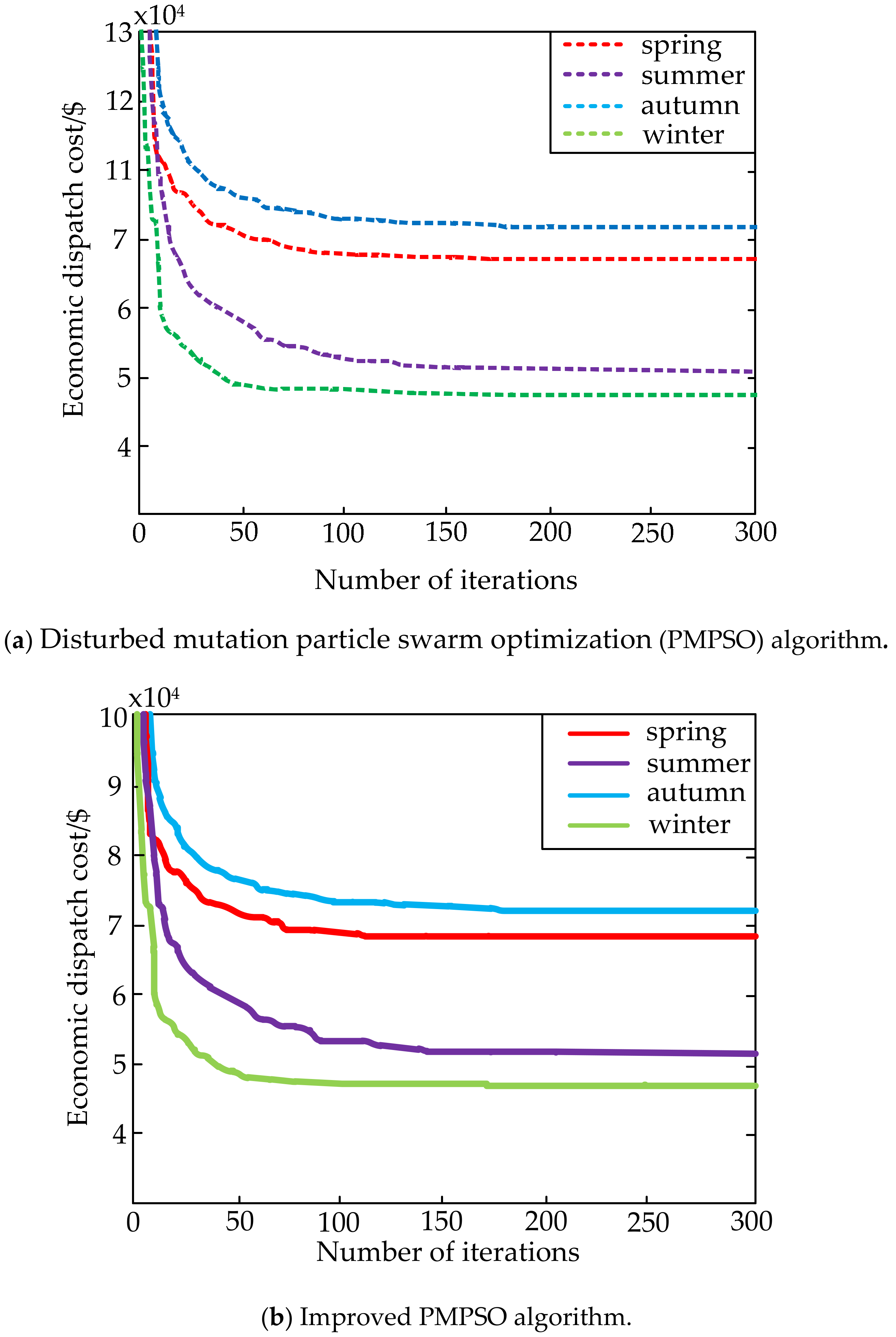
We used the disturbed mutation particle swarm optimization (PMPSO) and the improved perturbed variation particle swarm optimization to solve models, which consider wind power systems with four important periods of the year, for the following analysis. In the process of solving the four dispatch days, the load is kept unchanged, and the change curve of the system comprehensive cost is shown in
Figure 5.
It can be seen from
Table 5 that the improved PMPSO algorithm improves the optimization speed and also improves the optimization precision.
As can be seen from
Figure 5, within the four typical scheduling days selected economic costs are monotonically decreasing and eventually converge to a minimum; this shows the reliability of the results obtained. Therefore, the comprehensive operation cost can be significantly reduced through reasonable scheduling of thermal power units, electric boilers, cogeneration unit, and wind power. It can also improve the consumption of wind power and the economy of grid-connected operation.
The value range of the green economy index is simply divided into three segments, which are 0 <
λ < 0.85, 0.85 <
λ < 1.15, and 1.15 <
λ; the scheduling analysis is performed for each index interval by mode 1. The results are visible in
Table 6. When 0.85 <
λ < 1.15, it is considered that the environmental and social benefits are coordinated; the minimum comprehensive cost is the most suitable range of economic dispatch value. In contrast, when 0 <
λ < 0.85, sacrificing part of the environmental benefits, pursuing greater social and economic benefits, wind power consumption decreased by 8.95% on average, and overall cost increased by an average of 4.8125 K
$, the coal consumption cost of the thermal power unit and cogeneration unit increases. The green certificate produced by wind power does not meet the government-defined quota, and additional certificates are required to complete the task, increasing the cost of green certificate transactions. When 1.15 <
λ, some social benefits are sacrificed in order to seek greater environmental benefits, and wind power consumption increased by 5.5175% on average and overall cost increased by an average of 6.9325 K
$, the coal consumption cost of thermal power units and cogeneration units is reduced. Although the amount of wind power consumption is increased, the large number of wind power grids makes the system require more spare capacity to cope with wind power uncertainty and randomness. Considering that the green economy index affects the results of the economic dispatch model, when the value range is 0.85 <
λ < 1.15, the economic dispatch model can find the optimal solution.
This paper makes a comparison between increasing the output constraint and not increasing the output constraint and it can be seen from
Figure 6 that the stability index of the generator set without increasing the output constraint is 63%, and after the output force constraint is increased, the stability index of the generator set is 75%. It can be obtained that the stability of the unit is greatly improved after increasing the output constraint of the unit. For power generation cost, after increasing the output constraint, coal consumption increased by 0.45%, and coal consumption value increased. However, the coal consumption function in the optimization model shows a static curve of the coal consumption of the generating set, which does not satisfy the dynamic adjustment process under the frequent fluctuation of the power output of the generating set. The actual coal consumption will increase greatly when the power generation unit frequently adjusts its output, resulting in frequent changes in operating conditions. According to the actual operation data of a power plant unit, it can be roughly estimated that the output fluctuation of 1 MW will increase the dynamic coal consumption by 0.02 t. Therefore, the coal consumption after the increase in the output of the thermal power unit should be low, and the output force does not increase the actual coal consumption. It can be seen that considering the power generation stability of the thermal power unit can effectively improve the operating efficiency of the unit.
Figure 7 shows the simulation of a system for the whole year. The stability of the thermal power unit is 83%, and the stability is improved by nearly 19%. It can be concluded that increasing the output constraints of thermal power units has significant economic benefits for actual production. Therefore, in this example, the output of the thermal power unit is increased.
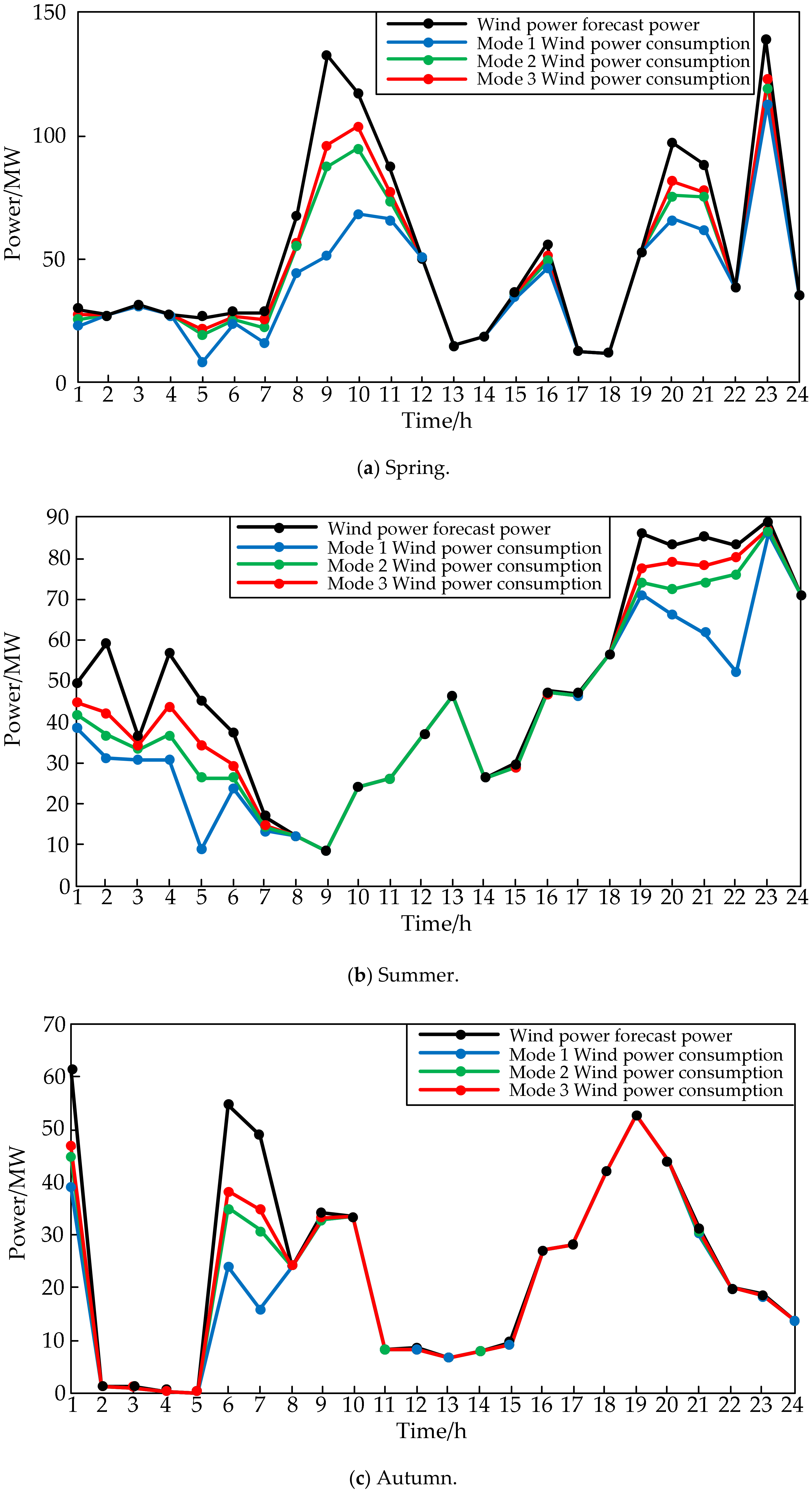
When the overall operating cost is the lowest, the amount of wind power consumption is shown in
Figure 8; the start-stop results of thermal power units are shown in
Table 7; the start-stop period of thermal power units is shown in
Table 8.
As can be seen from
Figure 8, wind power output exhibits a certain degree of randomness and volatility, and at the same time presents a certain degree of antipeaking. The wind power within the four dispatch days has a certain amount of wind abandon power that mainly occurs in the early morning and late night hours. At this stage, wind power output is larger, but the load demand is lower. To ensure the balance of power supply and demand in the operation of the power grid, a certain wind abandonment phenomenon occurs.
From
Table 7, it can be seen that the shutdown of the thermal power unit during operation has occurred, and the number of starts and stops is within the maximum number of unit limits, which ensures the normal operation of the unit.
Table 8 shows the time when the unit starts and stops, it can be seen that the start and stop of the unit mainly occur from 0:00 to 5:00. At this time, the load is at a low level, but the wind power output is higher. To increase the power of wind power, shutting down the unit with operational constraints allowed to reduce the output of thermal power units.
To verify the superiority of the transaction cost of the green certificate, the cost of the electric boiler, and the cogeneration unit in this paper, it is compared with the traditional dispatch method. When the green economic indicator is 0.85 <
λ < 1.15, the comparison results are shown in
Table 9 and
Table 10.
It can be seen from
Table 9 that under different scheduling modes, the pollutant emission will decrease first and then change with the increase of wind power on-grid. It indicates that the grid-connected consumption of wind power can reduce the output of thermal power units, thereby reducing pollutant emissions. However, when the capacity of the wind farm increases to the limit of consumption, the amount of wind power consumption remains unchanged, and the amount of pollutants discharged remains unchanged. In the same situation of wind power on-grid, Model 1 emits less pollutants than the other two scheduling models, which is more beneficial to the environment.
As can be seen from
Table 10, model 1 has the lowest overall cost in terms of overall cost. Regarding overall costs, after the electric boiler and the cogeneration unit are added to model 1, the wind power is further absorbed, the cost of thermal power is reduced, and the cost of wind power is increased. Under the influence of the green certificate trade, the increase of green economy indicators has played an important role in balancing the green economy and social economy. Although the start-up and shutdown of the thermal power unit in model 1 caused a start-stop cost, it can significantly reduce the output of the thermal power unit, reduce the environmental cost caused by the thermal power unit, increase the amount of wind power consumption, and reduce the cost of the green certificate.


