Improving Control Efficiency of Dynamic Street Lighting by Utilizing the Dual Graph Grammar Concept

Abstract

The paper introduces a definition of dual graph grammar. It enables two graphs to share information in a synchronized way. A smart city example application, which is an outdoor lighting control system utilizing the dual graph grammar, is also demonstrated. The system controls dimming of street lights which is based on traffic intensity. Each luminaire’s light level is adjusted individually to comply with the lighting norms to ensure safety. Benefits of applying the dual graph grammar are twofold. First, it increases expressive power of the mathematical model that the system uses. It becomes possible to take into account complex geographical distribution of sensors and logical dependencies among them. Second, it increases the system’s efficiency by reducing the problem size during run-time. Experimental results show a reduction of the computation time by a factor of 2.8. The approach has been verified in practice.

1. Introduction

Applying the graph theory to create formal models of intelligent spaces has already been proven useful, as they enable interactions between smart city components [1,2]. Synergy of knowledge regarding different aspects of the space under consideration can result in added value [3]. An illustrative example is street and road lighting [4]. A formal architectural model can represent features such as streets, pavements, sidewalks, medians, buildings, trees etc. Having such a model enables outdoor lighting design optimization and its dynamic control [1].

Lighting design is about defining the placement of poles and luminaires as well as their parameters, such as luminaire type, its power, overhang, tilt, rotation etc. Design optimization is aimed at providing particular values of these parameters to maximize safety and minimize energy usage.

Dynamic control is about adjusting lighting levels on demand, based on the current needs, taking into account such factors as traffic intensity or weather conditions. Having a graph-based formal model enables easy deployment of control schemas, even exceedingly sophisticated ones. It follows the idea of data-driven design which separates data, the formal model, from its processing, the control rules. From a practical point of view, it also facilitates deployments in new locations. The control rules do not have to be updated or reprogrammed—it is sufficient to provide a new model of the environment. Such graph-based dynamic control results in increased efficiency, both in terms of lighting energy consumption reduction and decreased deployment effort.

In order to make the environment safe, its illumination has to comply with lighting norms, such as CEN/TR 13201-1: 2004 or 2014 [5,6]. While designing a lighting system, proper selection of the lighting class, applied to a given area being illuminated, is most important. A lighting class is a set of lighting requirements such as illumination, uniformity etc. Particular classes, such as me2, me3 etc. deliver well-defined lighting levels.

The main driver for this paper is based on experience from a research project which resulted in deployment of 3768 light points in Kraków, Poland. It has been observed that the sensor infrastructure becomes more and more complex, delivering more and more information. It is often redundant to provide comparative results or robustness to failures. In Kraków, the number of ambient light sensors for outdoor lighting has increased 15 times over just one year (2016). Instead of a single sensor in an electric cabinet which supplies three circuits of 50 luminaires each, there is one for every 10 luminaires, mounted on the lamp pole. Similarly, the number of traffic intensity sensors has increased as well. For a typical intersection, the number of traffic intensity detectors (induction loops) has increased by a factor of 2. For example, in the case of a 4-way intersection with 10 inbound and 6 outbound lanes, it has increased from 10 to 20.

This paper focuses on providing a formal basis to incorporate knowledge regarding multiple sensors into the lighting control model by introducing the dual graph grammar concept. As a result, the model remains easy to comprehend, while the computing power needed to process and interpret it is decreased.

2. Motivation and Related Research

The concepts of smart cities and smart environments, as well as technologies related to them, are gaining traction. The main technological enablers are Internet of Things (IoT) and sensor nets resulting in broad availability of data [4,7,8]. The main drivers are safety, convenience and, last but not least, economic factors such as energy savings [9,10]. Often, combination of smart technologies with renewable energy sources offers added economic value [11]. Such solutions can be applied at the scale of an entire city [12], a single block, or indoor [13,14,15]. They are often based on rules and configured for particular deployments [16,17,18,19]. However, a lack of underlying formal models often results in harder and more costly adjustment to evolving requirements or deployment at new locations.

Graphs seem to be an appropriate tool to develop such models [1,20]. However, one of the challenges is the efficiency of graph transformations. The main problems are graph parsing and determination of membership. With strong limitations on the graph structure, the membership problem is of $O\left(n^2\right)$ computational complexity [21]. However, in general it remains a higher-order polynomial. The efficiency depends on the size of the entire graph. One of the methods of its reduction is the concept of hierarchical graphs [22,23], where the nodes can also be graphs introducing more detail at the graph’s lower levels. While the concept provides a convenient structure, it also increases the graph size and processing complexity. Real-world cases indicate a need for a representation which would not require increased processing power. An example of such a case is generation of dynamic control rules for an outdoor lighting system. Initially, a flat graph structure, the Control Availability Graph (CAG), was proposed for this purpose [1,20]. It is an extract of architectural features that are necessary to provide dynamic control, hence the name. Dynamic control is provided by software performing the following tasks:

• obtaining data from sensors and updating the CAG accordingly (traffic intensity and ambient light intensity sensors are considered),
• firing the control rules in the form of graph transformations, which results in conclusions being stored in the CAG,
• delivering the conclusions to the actuators, which set power levels of the appropriate luminaires.

The more luminaires are under control, the larger the CAG becomes. Since the control software is meant to be used as an embedded system, the performance requirements play a major role.

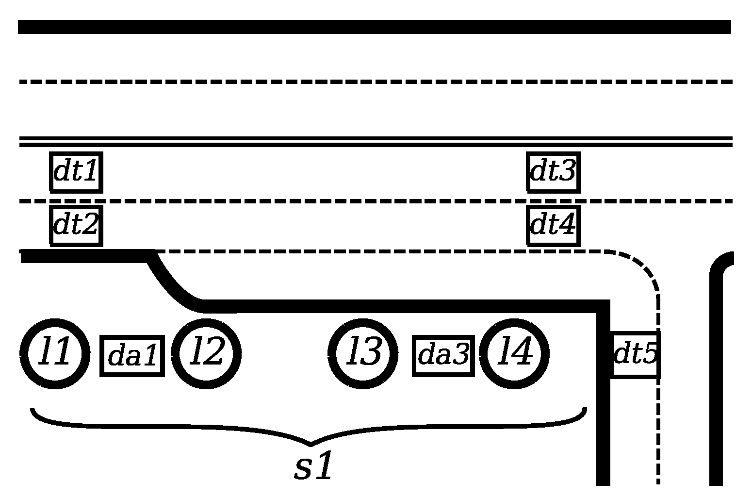
To present the CAG concept let us introduce an example intersection which is given in Figure 1. To control lighting intensity, the following formal structure has been defined. There is a single street segment $s1$, which is a length of a street with uniform lighting conditions. It covers four luminaires $l1,\dots ,l4$. There is also an ambient light detector $da1$ and a traffic intensity detector $dt1$. A corresponding CAG is given in Figure 2. Some of the graph indices, labels and attributes are shown. The following graphical convention is used. Vertex labels are indicated within vertices, indices, if present, are prefixed with a “/” character. For example, a vertex indicated as $dt/dt1$ has the label $dt$ and an index of $dt1$. In this case, the vertex represents a traffic intensity detector, hence the label $dt$. Indices are arbitrary symbols to increase readability and correspondence with real objects. Edge labels can also be present. For example, between vertices $s1$ and $c1$, there is a label indicating the lighting class $me3$. Attribute names and values are indicated as well, for example $p\left(0.8\right)$ is an attribute p holding the value of $0.8$ which indicates luminaire’s power level.

The graph consists of a vertex labeled as $dt$ which represents a traffic intensity detector, $da$ which represents an ambient light detector, s which represents a segment, c which represents a luminaire configuration, and finally l representing a luminaire. Edge labels between vertices c and s represent lighting classes which are provided by a given configuration on a given segment. With each lighting class, the power level of the luminaries belonging to the segment is defined. It is represented as the p attribute of an edge between vertices labeled c and l. Its value is a coefficient by which a luminaire’s power setting has to be adjusted, ranging from 0 (0%) to 1 (100%). It indicates how much the luminaire should be dimmed. Assuming that the power setting is expressed as $p\left(x\right)$, its relationship with the dimming is expressed as: $x=1-d$. The settings for a given configuration which supports an indicated norm are computed based on photometric calculations according to the lighting norms while building the graph. During run-time, when control is carried out, the values of the sensors allow to determine the proper lighting class, represented as an edge between s and c. The power settings for each of the luminaires are selected accordingly based on the class.

In case of cities with thousands of lamps, such a graph consists of hundreds of thousands of nodes and edges, thus both the readability of the model and efficiency of graph grammars are major challenges.

The CAG is built by performing photometric calculations based on the lighting norms. The examples in this paper, as well as the deployment in Kraków, utilize CEN/TR 13201-1: 2004 norm [5] even though the norm was updated in 2014 [6]. It is because the deployment was designed in 2015 and 2016 at which time the 2014 update was not acknowledged in Poland yet.

In this paper, we introduce the dual graph grammar concept. It results in a graph-based model with low computational complexity and flexibility where needed. An example application is a dynamic street lighting control system. It enables efficient adjustment of lighting to particular needs and capabilities by providing high-performance processing. The adjustment can be based on far more complex logical relationships among sensors than the ones presented in Figure 2.

There is also additional motivation to use as many sensors as available. The more sensor information is available, the more precise the control process is, which can lead to increased energy savings. For example, if there are redundant traffic intensity sensors taken into consideration, not delivering the measurements by one of them does not influence the control process. If there is no redundancy, a malfunctioning traffic detector forces the control system to assume the maximum value of allowed traffic intensity. This results in delivering more light than necessary and consuming more energy.

It needs to be pointed out that even insignificant energy savings at a single luminaire lead to substantial savings for a city, due to the effect of scale. A city with a population of 1 million has approximately 80,000 light points (it has been experimentally established that there is a relationship between population density and the number of light points in urbanized areas, there are 8 light points per 100 citizens for Poland), which consume from 20 to 50 GWh per year. The estimation is based on the assumption that the wattage of a single luminaire varies from 60 to 150 (both LED and HPS light sources) on average.

3. Problem Statement

A synthesis of the CAG model, which is based on photometric calculations and a rule-based control approach were proposed in [1]. The control process works efficiently as long as the sensor infrastructure is built from the ground up, having only one detector of a given kind at any street segment. However, in the real world, there are usually multiple detectors of a kind at one segment which are part of an Intelligent Transportation System (ITS) or a sensor network which is already deployed. If so, input to the lighting control system should be based on a result of calculations on data from these multiple detectors. Extending the model, thus the graph grammar, to cover these additional computations, while perfectly justified, leads to some undesired side effects. First of all, the model becomes less clear, focusing on the sensors and relationships between them, instead of binding sensors with segments, configurations and luminaires. Then, the control rules have to take care of choosing the most appropriate sensor from a group and applying the appropriate calculations. It makes them more complex, challenging to verify, and can also lead to decreased processing performance of such a model during run-time.

To handle these issues, the concept of a dual graph grammar is introduced. Such a grammar provides double expressiveness of the model: efficient calculations on sensor data and logical organization of the infrastructure. It is created by combining two separate graph grammars and explicitly stating the synchronization conditions between the graphs they generate. As a result, there will be two synchronized graphs representing these two aspects. Such an approach will also improve run-time performance, since the two graphs can be processed independently.

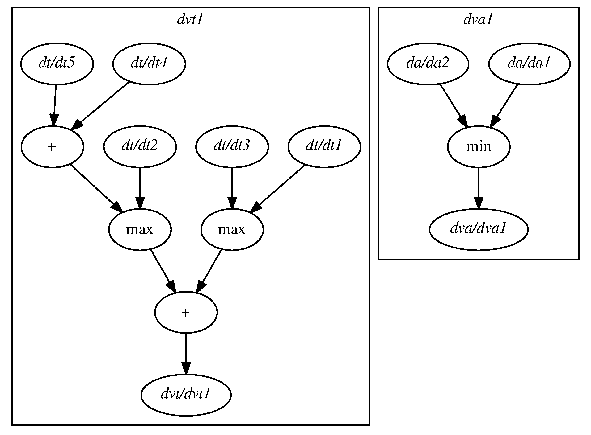
Before introducing formal definitions, let us focus on an example which explains the problem. As mentioned earlier, in highly urbanized areas, the example shown in Figure 1 becomes unrealistic. The actual detector distribution would be close to that presented in Figure 3 instead. The difference is that for multi-lane streets, there is usually at least one detector per lane. Sometimes, the traffic intensity detectors are doubled or tripled and their placement could be before or after an intersection. Considering the example in Figure 3, in order to calculate the traffic intensity $dt$ in segment $s1$, one needs to perform:

$$dt=\max (dt1,dt3)+\max (dt2,(dt4+dt5\left)\right)$$

where $dt1,\dots ,dt5$ express traffic intensity measured by respective traffic intensity detectors. In this case, $dt1$ and $dt3$ are redundant, measuring traffic intensity in the same lane. Similarly, $dt2$ and a sum of $dt4$ and $dt5$ are redundant too.

There could also be more than one ambient light sensor for a single segment. These sensors are often located on the poles, together with luminaires. The actual ambient light intensity, taking into account multiple ambient light detectors, should be calculated as:

$$da=\min (da1,da2)$$

where $da1$ and $da2$ represent ambient light intensity measured by respective detectors. The min() function is used since the lighting level at the segment has to be adjusted to the lowest value of ambient light detected, to avoid the segment being underlit.

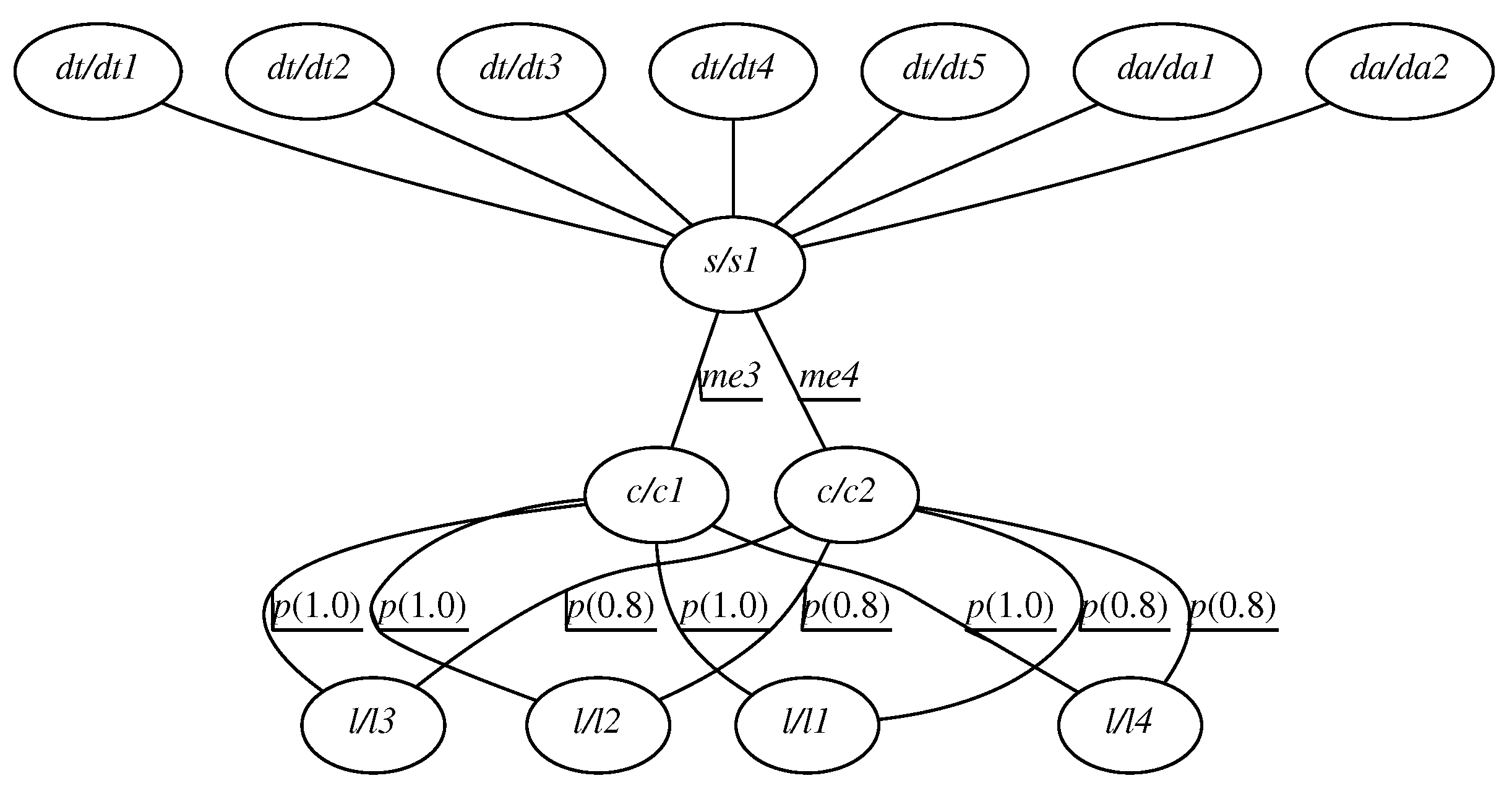
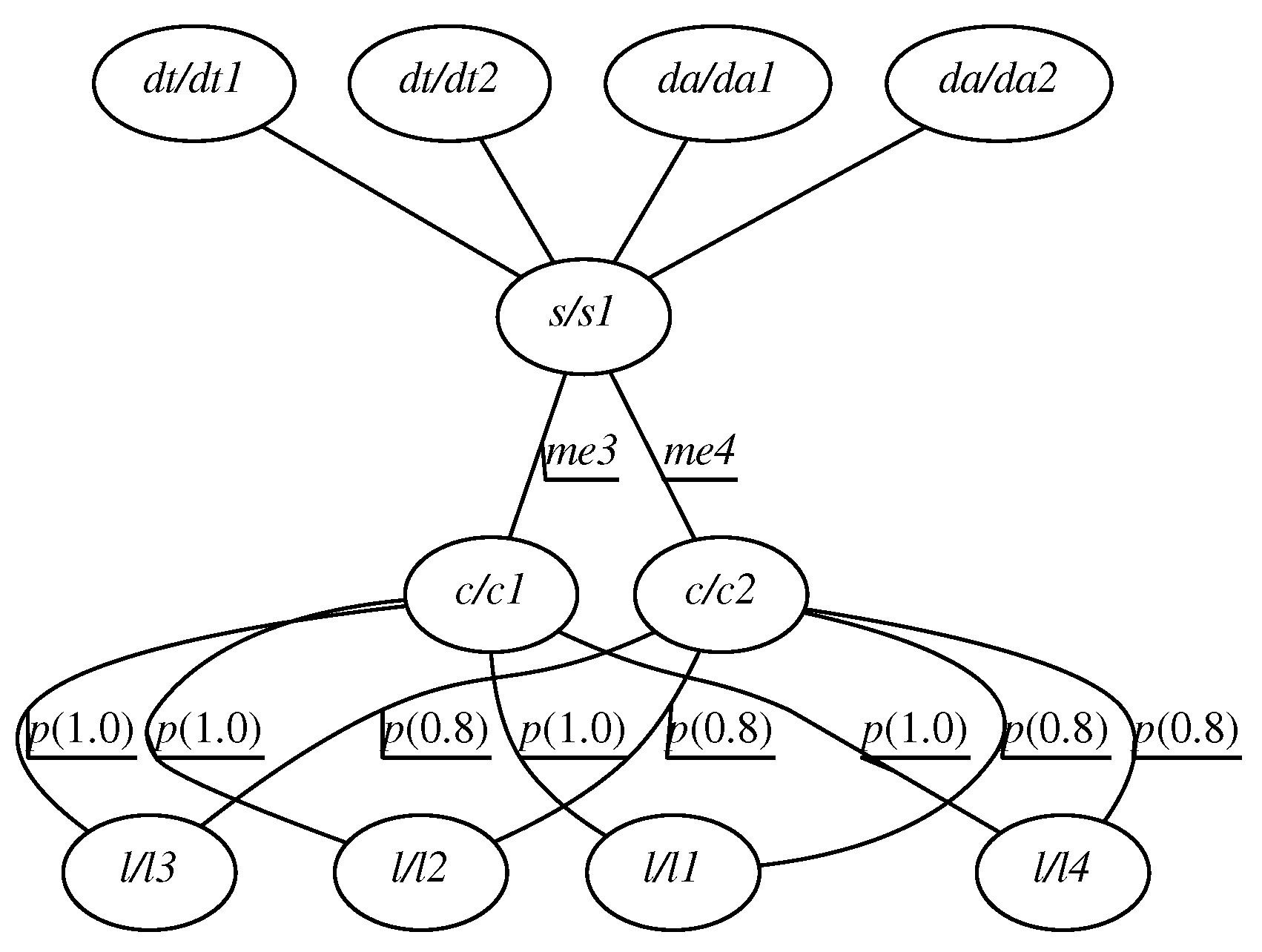
A model with all the sensors taken into consideration could look like the one given in Figure 4. However, as mentioned earlier, it is not practically feasible, because it lacks the knowledge about what particular calculations should be performed; spatial and logical relationships among the detectors are not there. Thus, in order to make it usable, the model gets simplified, taking into consideration only a subset of the detectors, as shown in Figure 5. Then, by a rule of thumb, traffic intensity for all traffic detectors should be added up, while ambient light intensity is calculated as a minimum over all detectors for a given segment.

However, there are still some issues:

• no detector redundancy is taken into consideration, which the increases risk of traffic intensity misjudgment due to sensor failure or noise,
• sensors to be included in the CAG have to be hand-picked,
• data aggregation from multiple detectors is driven by control rules; it is performed on an arbitrary number of detectors, which might result in run-time performance degradation, since the number of detectors can vary from segment to segment.

Let us show how the proposed dual graph grammar can solve these issues.

4. Dual Graph Grammar Representation

As mentioned in the previous section, the CAG structure does not directly represent the complexity of the influence of multiple sensors on lighting segments and subsequently on the luminaires to be controlled. Hard-coding it, which is using general-purpose programming languages to represent this influence, would make it hard to analyze or modify, since it would not be part of the graph. On the other hand, extending the CAG to perform additional processing to cover the influence would increase its size and decrease the overall processing efficiency, since the complexity of graph parsing algorithms depends on the graph size. To solve these problems, we introduce the dual graph grammar representation, in which two graph grammars are used to generate a consistent model in such a way that they are separate graphs with common elements. The synchronization of both graphs is provided by the validation properties associated with each of the grammars. As a result, the two graphs have separate purposes: one is used for control, and the other—to express relationships among sensors. Let us define this structure formally.

Definition 1.

A dual graph grammar $[\mathsf{\Psi },\Theta ]$ is a pair of graph grammars:

$$\mathsf{\Psi }=({\mathsf{\Sigma }}_{\mathsf{\Psi }},{\Gamma }_{\mathsf{\Psi }},{\Delta }_{\mathsf{\Psi }},{\mathsf{\Phi }}_{\mathsf{\Psi }},S_{\mathsf{\Psi }},{\mathsf{\Pi }}_{\mathsf{\Psi }})$$

$$\Theta =({\mathsf{\Sigma }}_{\Theta },{\Gamma }_{\Theta },{\Delta }_{\Theta },{\mathsf{\Phi }}_{\Theta },S_{\Theta },{\mathsf{\Pi }}_{\Theta })$$

where:

• ${\mathsf{\Sigma }}_{\mathsf{\Psi }}$ and ${\mathsf{\Sigma }}_{\Theta }$ are the sets of node labels,
• ${\Delta }_{\mathsf{\Psi }}\subset {\mathsf{\Sigma }}_{\mathsf{\Psi }}$, ${\Delta }_{\Theta }\subset {\mathsf{\Sigma }}_{\Theta }$ are the sets of terminal node labels,
• ${\Gamma }_{\mathsf{\Psi }}$ and ${\Gamma }_{\Theta }$ are the sets of edge labels,
• ${\mathsf{\Phi }}_{\mathsf{\Psi }}$ and ${\mathsf{\Phi }}_{\Theta }$ are the sets of transformation rules,
• $S_{\mathsf{\Psi }}$ and $S_{\Theta }$ are the starting graphs,
• ${\mathsf{\Pi }}_{\mathsf{\Psi }}$ and ${\mathsf{\Pi }}_{\Theta }$ are the validation graph grammar conditions,

and the following condition is fulfilled: ${\mathsf{\Sigma }}_{\mathsf{\Psi }}\cap {\mathsf{\Sigma }}_{\Theta }\ne ⌀$.

Applications of transformation rules on a graph are atomic. This means that two productions on a single subgraph are mutually exclusive.

Definition 2.

A dual graph grammar $[\mathsf{\Psi },\Theta ]$ is synchronized if both validation conditions ${\mathsf{\Pi }}_{\mathsf{\Psi }}$ and ${\mathsf{\Pi }}_{\Theta }$ are met.

Let us explain how the proposed dual graph grammar notation supports the problem of maintaining the influence of multiple sensors on a given segment. The basis for this concept is the notion of a virtual detector. It represents a data source with values calculated based on information from actual detectors. There is only one virtual detector of a given type in relation with a segment. In this case, a node labeled by $dva$ will represent such a detector, providing ambient light intensity. Similarly, a node labeled by $dvt$ (virtual traffic detector) will represent traffic intensity. We assume that $dva$ and $dvt$ are the only node labels that belong to ${\mathsf{\Sigma }}_{\mathsf{\Psi }}\cap {\mathsf{\Sigma }}_{\Theta }$.

The $\mathsf{\Psi }$ graph grammar will provide the logical relationships among entities; it enables control by defining a new Control Availability Graph: CAG${}_{\mathsf{\Psi }}$. Its role is to:

• maintain information about the lighting infrastructure to be controlled,
• optimize the internal structure of the lighting system (for more details see [24]),
• evaluate the current CAG${}_{\mathsf{\Psi }}$ parameters to provide actual control.

The $\Theta$ grammar will define the evaluation rules for virtual detectors—a Detector Structure Graph (DSG${}_{\Theta }$). Its role is to:

• maintain information about the detectors’ logical structure and evaluation conditions of sensory data resulting in virtual detectors’ values,
• evaluate the virtual detectors’ values.

Let us define CAG${}_{\mathsf{\Psi }}$ and DSG${}_{\Theta }$ formally.

Definition 3.

CAG${}_{\mathsf{\Psi }}$ is an attributed graph over the set of node labels ${\mathsf{\Sigma }}_{\mathsf{\Psi }}$ and the set of edge labels ${\Gamma }_{\mathsf{\Psi }}$ which is generated by the Ψ grammar:

$${\mathit{CAG}}_{\mathsf{\Psi }}=(V_{\mathsf{\Psi }},E_{\mathsf{\Psi }},la{b}_{\mathsf{\Psi }}^V,la{b}_{\mathsf{\Psi }}^E,{\mathsf{\Sigma }}_{\mathsf{\Psi }},{\Gamma }_{\mathsf{\Psi }},at{t}_{\mathsf{\Psi }}^V,at{t}_{\mathsf{\Psi }}^E,A_{\mathsf{\Psi }}^V,A_{\mathsf{\Psi }}^E)$$

where:

• $V_{\mathsf{\Psi }}$ is a finite, nonempty set of graph nodes identified unambiguously by some injective indexing function $Index:V_{\mathsf{\Psi }}\to \mathit{IS}$, where $\mathit{IS}$ is a set of indexing symbols (usually $\mathbb{N}$ is used but in some cases it is easier to provide arbitrary symbols to increase readability),
• $E_{\mathsf{\Psi }}\subseteq V_{\mathsf{\Psi }}\times V_{\mathsf{\Psi }}$ is a set of edges,
• $\mathsf{\Psi }\_la{b}_{\mathsf{\Psi }}^V:V_{\mathsf{\Psi }}\to {\mathsf{\Sigma }}_{\mathsf{\Psi }}$ is a node labelling function,
• $\mathsf{\Psi }\_la{b}_{\mathsf{\Psi }}^E:E_{\mathsf{\Psi }}\to {\Gamma }_{\mathsf{\Psi }}$ is an edge labelling function,
• ${\mathsf{\Sigma }}_{\mathsf{\Psi }}=\{s,l,dvt,dva,c\}$ is a set of node labels, where:

  -

  s represents segments,

  -

  l represents luminaires,

  -

  $dvt$ and $dva$ represent virtual traffic and ambient light intensity detectors, respectively,

  -

  c represents a configuration, which is a set of adjustments, associated with a relevant set of luminaires at a given segment,

• ${\Gamma }_{\mathsf{\Psi }}=\{me2,me3,me4,me5\}$ is a set of edge labels, where: $me2$, $me3$, $me4$, $me5$ are lighting classes,
• $at{t}_{\mathsf{\Psi }}^V:V_{\mathsf{\Psi }}\times {\mathsf{\Sigma }}_{\mathsf{\Psi }}\to 2^{A_{\mathsf{\Psi }}^V}$ is a node attributing function, such that for $x\in V_{\mathsf{\Psi }}, l\in {\mathsf{\Sigma }}_{\mathsf{\Psi }}, a\in A_{\mathsf{\Psi }}^V at{t}_{\mathsf{\Psi }}^V(x,l)\left(a\right)$ is a value of the attribute a,
• $at{t}_{\mathsf{\Psi }}^E:E_{\mathsf{\Psi }}\times {\Gamma }_{\mathsf{\Psi }}\to 2^{A_{\mathsf{\Psi }}^E}$ is an edge attributing function, such that for $x\in E_{\mathsf{\Psi }}, l\in {\Gamma }_{\mathsf{\Psi }}, a\in A_{\mathsf{\Psi }}^{E}at{t}_{\mathsf{\Psi }}^E(x,l)\left(a\right)$ is a value of the attribute a,

Intuitively, we feel that each segment s is connected by an edge with exactly one $dvt$ and one $dva$.

Formally, the validation condition ${\mathsf{\Pi }}_{\mathsf{\Psi }}$ of the grammar is as follows:

$$\begin{array}{cc}\hfill \forall v_1,\in V_{\mathsf{\Psi }}:la{b}_{\mathsf{\Psi }}^V\left(v_1\right)=& l,\hfill \\ \hfill \exists !v_2,\in V_{\mathsf{\Psi }}:la{b}_{\mathsf{\Psi }}^V\left(v_2\right)=& dvt,\hfill \\ \hfill \exists !v_3,\in V_{\mathsf{\Psi }}:la{b}_{\mathsf{\Psi }}^V\left(v_3\right)=& dva,\hfill \\ \hfill \exists v_4\in V_{\mathsf{\Psi }}:la{b}_{\mathsf{\Psi }}^V\left(v_4\right)=& s,\hfill \\ \hfill \exists v_5\in V_{\mathsf{\Psi }}:la{b}_{\mathsf{\Psi }}^V\left(v_5\right)=& c,\hfill \\ \hfill \{(v_3,v_4),(v_2,v_4),(v_4,v_5)(v_5,v_1)\}\subset & E_{\mathsf{\Psi }}\hfill \end{array}$$

(1)

Definition 4.

DSG${}_{\Theta }$ is an attributed directed graph over the set of node labels ${\mathsf{\Sigma }}_{\Theta }$ and the empty set of edge labels ${\Gamma }_{\Theta }$ which is generated by the Θ grammar:

$${\mathit{DSG}}_{\Theta }=(V_{\Theta },E_{\Theta },la{b}_{\Theta }^V,{\mathsf{\Sigma }}_{\Theta },at{t}_{\Theta }^V,A_{\Theta }^V)$$

where:

• $V_{\Theta }$, $E_{\Theta }$, $la{b}_{\Theta }^V$, $at{t}_{\Theta }^V$, $A_{\Theta }^V$ are defined similarly as in Definition 3,
• ${\mathsf{\Sigma }}_{\Theta }=\{dvt,dva,dt,da,+,-,\times ,/,min,max,val\}$ is a set of node labels, where:

  -

  $dvt$ and $dva$ represent virtual traffic and ambient light intensity sensors, respectively,

  -

  $dt$ and $da$ represent actual traffic and ambient light intensity sensors, respectively,

  -

  $+,-,\times ,/,min,max$ represent arithmetic operators,

  -

  $val$ represents constant arbitrary values.

Formally, the validation condition ${\mathsf{\Pi }}_{\Theta }$ makes sure that there are no non-terminals in the graph:

$$\forall v\in V_{\Theta }:la{b}_{\Theta }^V\left(v\right)\in {\Delta }_{\Theta }$$

(2)

While DSG${}_{\Theta }$ is being built there may be vertices with labels being-non terminals. In such a case, the graphs are not in a synchronized state since according to Definition 2, the validation conditions are not met.

5. Solving the Problem

To summarize, in order to handle the issues presented in Section 3, the following assumptions are made. There is a dual graph grammar $[\mathsf{\Psi },\Theta ]$ defined. The $\mathsf{\Psi }$ graph grammar is used to represent the control structure of the lighting system stored in a CAG${}_{\mathsf{\Psi }}$. The $\Theta$ graph grammar represents the evaluation of virtual sensors, defined by a DSG${}_{\Theta }$.

As a result, the following proposals can be made:

p1

the model of the dynamic lighting control is a graph, which consists of: CAG${}_{\mathsf{\Psi }}$ and DSG${}_{\Theta }$,

p2

there are virtual detectors introduced, represented by the graphs’ synchronization vertices,

p3

there is only a single virtual detector of a given type (traffic, ambient light, etc.) in relation to an individual segment,

p4

logical relationships between detectors and a virtual detector are expressed as a graph.

Application of the proposed dual graph grammar has the following properties:

• it separates the logical relationships between segments, detectors and luminaires from calculations on sensor data; thus, control is separated from evaluation and both can be processed separately during run-time,
• it simplifies the control process graph transformations, since there is only one edge between a segment and a detector of a given kind,
• a detector can be used in calculations for multiple virtual detectors,
• there is a number of vertices to be processed upon executing control being reduced, since only the $\mathsf{\Psi }$ graph is considered; this enhances run-time performance of the control system,
• full knowledge necessary for control is expressed as a graph, subject to analysis and validation,
• formal graph folding enables extracting and viewing a CAG${}_{\mathsf{\Psi }}$ or a DSG${}_{\Theta }$, allowing for a clear representation of control availability or logical relationships among detectors, respectively,
• high-performance processing of DSG${}_{\Theta }$ is possible since it represents a parse tree,
• calculations (DSG${}_{\Theta }$) can be easily updated without influencing CAG${}_{\mathsf{\Psi }}$,
• control availability (CAG${}_{\mathsf{\Psi }}$) can be easily updated without influencing DSG${}_{\Theta }$.

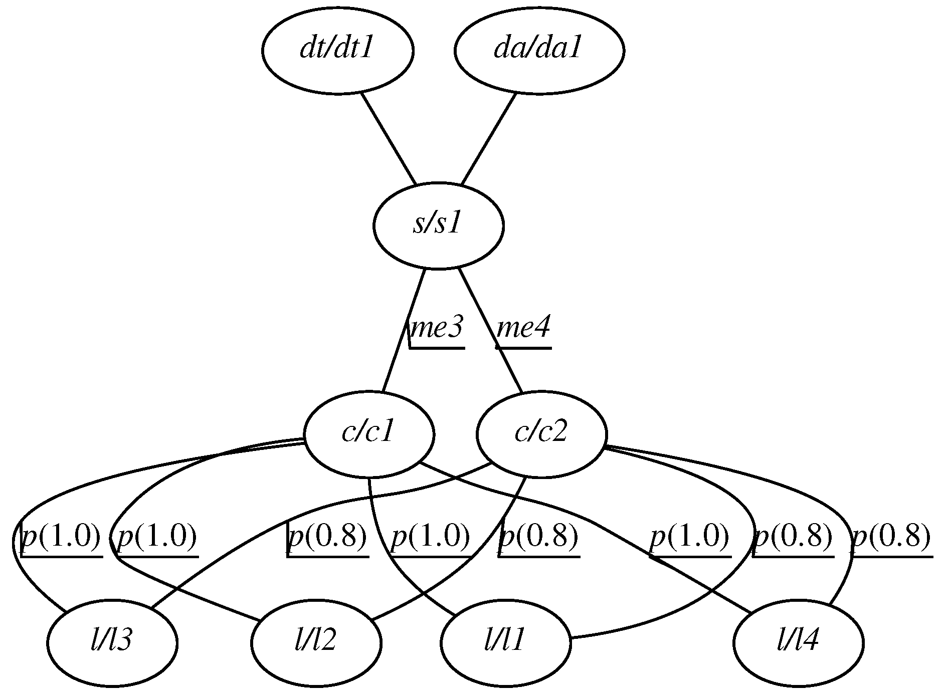
Applying the proposed dual graph grammar approach to the example in Figure 3 results in a model presented in Figure 6 (CAG${}_{\mathsf{\Psi }}$) and Figure 7 (DSG${}_{\Theta }$).

6. A Real World Example

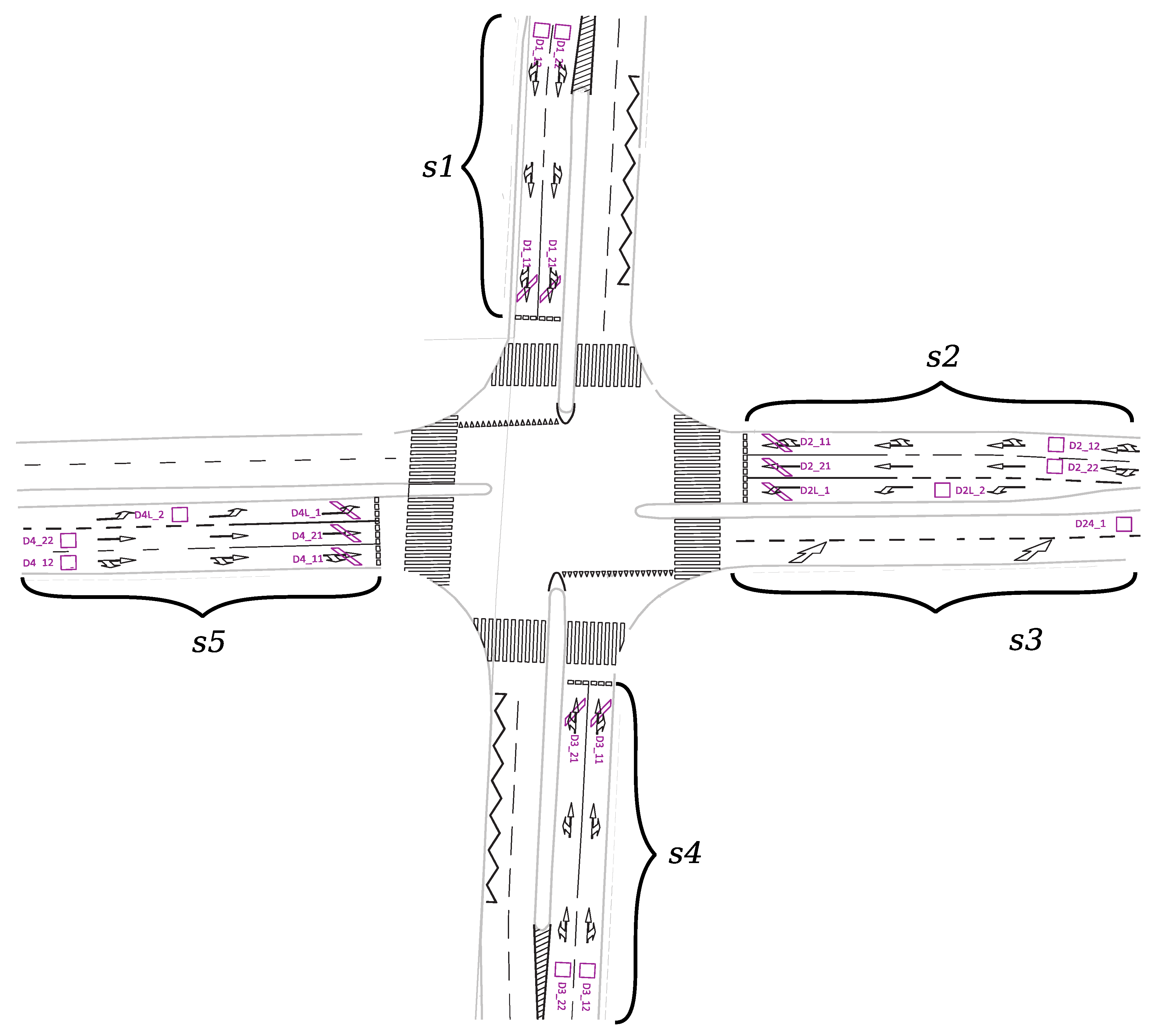
Having defined the approach, let us present an intuitive real world example. It is an excerpt from a large-scale deployment of dynamic lighting control system in Krakow, Poland. The excerpt describes a single intersection presented in Figure 8. There are five segments: $s1$, $s2$, $s3$, $s4$, $s5$. The intersection is equipped with inductive loop traffic intensity sensors: $D2\_11$, $D2\_12$, $D2\_21$, $D2\_22$, $D4L\_2$, $D4L$, $D4\_22$, $D4\_21$, $D4\_12$, $D4\_11$, $D3\_11$, $D3\_12$, $D3\_21$, $D3\_22$, $D1\_12$, $D1\_11$, $D1\_22$, $D1\_21$, $D24\_1$. There are no other detectors considered.

Influence of traffic data from the virtual detectors on particular segments, assignments of lamps ($l1,\dots ,l14$) to the segments as well their configurations ($c1,\dots ,c6$)—represented in CAG${}_{\mathsf{\Psi }}$—are shown in Figure 9. Since there are no luminaires under control in $s1$ and $s5$, there is no edge connecting $s1$ or $s5$ with any vertex labeled with c. The ambient light detectors are omitted for simplicity, so the available $CA{G}_{\mathsf{\Psi }}$ vertex labels are defined as: $L_V=\{s,l,dvt,c\}$. Furthermore, ${\Gamma }_{\mathsf{\Psi }}=\{me3c,me4b,me5\}$ since the set of lighting classes is adjusted to cover $me3c$, $me4b$, $me5$. There are classes $me4b$ and $me5$ available on the segment $s4$, while $me3c$ and $me4b$ are available on $s2$ and $s3$. These lighting classes were selected due to physical features of the segments according to the lighting norms. Correspondence between lighting classes and the power settings of the luminaires have been verified by using photometric calculations. Similarly, the synchronization condition ${\mathsf{\Pi }}_{\mathsf{\Psi }}$ is relaxed, due to a lack of ambient light detectors:

$$\begin{array}{cc}\hfill \forall v_1,v_2\in L_V:la{b}_V\left(v_1\right)=l,la{b}_V\left(v_2\right)=& dvt\hfill \\ \hfill \exists v_4\in L_V:la{b}_V\left(v_4\right)=& s,\hfill \\ \hfill \exists v_5\in L_V:la{b}_V\left(v_5\right)=& c,\hfill \\ \hfill \{(v_2,v_4),(v_4,v_5)(v_5,v_1)\}\subset & E\hfill \end{array}$$

(3)

For each of the configurations, for the given class, there are lamp settings defined as edges between c and l. They indicate power setting for a particular lamp, provided by a value of attribute p. For example, there is an edge between $s4$ and $c5$, which represents a configuration for establishing the $me4b$ lighting class on $s4$. It is carried out by setting the luminaires $l6$–$l4$ to full power, which is indicated by the attribute p set to $1.0$ ($p\left(1.0\right)$). For comparison, establishing the $me5$ class on the same segment would set the luminaires to 80% (p(0.8)). The actual power settings were computed by running photometric calculations while building CAG${}_{\mathsf{\Psi }}$.

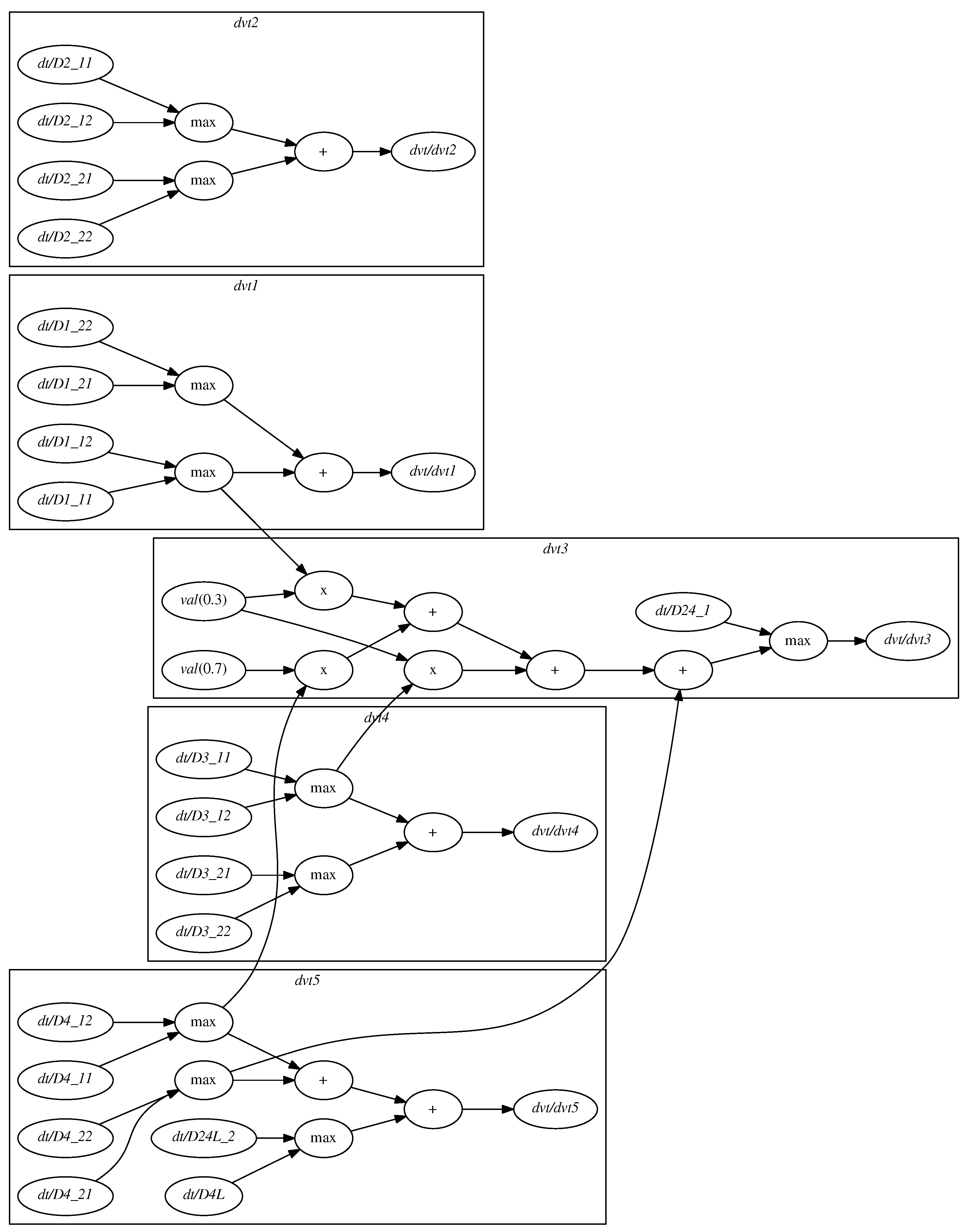
The DSG${}_{\Theta }$ part, which represents virtual sensor evaluations, is presented in Figure 10. The disconnected directed graph forms arithmetic expression parse trees. As a visual aid, the vertices representing the sensors ($dv$ label) that are placed in the same segment as the virtual sensor are additionally enclosed in solid lines labeled with the virtual sensor index. For example, there is a virtual sensor $dvt2$ which belongs to the same segment as the detectors $D2\_11$, $D2\_12$, $D2\_21$, $D2\_22$, thus it is enclosed by a solid line labeled $dvt2$. Nodes representing arithmetic functions are labeled with their respective symbols e.g., max, +, × etc. The value of $dvt2$ is evaluated as: max$(D2\_11,D2\_12)+\max (D2\_21,D2\_22)$. There are also vertices representing constants; their values are indicated using $val$ attributes. For example, there are two nodes attributed $val\left(0.3\right)$ and $val\left(0.7\right)$ in the enclosure $dvt3$. Their respective values are used for evaluation of $dvt3$, which is a result of: max$(D24\_1,\max (D1\_12,D1\_11)\times 0.3+0.7\times \max (D4\_12,D4\_11)+0.3\times \max (D3\_11,D3\_12)+\max (D4\_22,D4\_21\left)\right)$. For this particular virtual detector, measurements provided by detectors in other segments are also taken into consideration, which increases the connectivity of the graph.

As a result, the size of CAG${}_{\mathsf{\Psi }}$, in comparison with CAG, is reduced. For the example intersection, considering all sensors, the CAG consists of 19 traffic intensity detectors ($dt$), 5 segments (s), 14 luminaires (l) and 6 configurations (c), which results in a total of 44 vertices. There are 21 edges between traffic detectors ($dt$) and segments (s), 6 edges between segments (s) and configurations (c), and 28 edges between configurations (c) and luminaires (l) which results in 55 edges total. For comparison, CAG${}_{\mathsf{\Psi }}$ consists of the following vertices: 5 virtual traffic intensity detectors ($dvt$), 5 segments (s), 14 luminaires (l) and 6 configurations (c), with a total of 30 vertices. There are the following edges: 5 between virtual traffic detectors ($dvt$) and segments (s), 6 between segments (s) and configurations (c), and 28 between configurations (c) and luminaires (l) which results in 39 total. The size of a graph is expressed as the number of its edges. In this case, it was reduced by 29%, from 55 to 39. The computational complexity of the dynamic control algorithms is $O\left(n^3\right)$. This is due to the properties of the $\mathsf{\Psi }$ grammar which do not comply with the limitations proposed in [21]. Therefore, the aforementioned graph size reduction decreases the number of computations performed during run-time from 166,375 to 59,319, giving a reduction factor of 2.8. Such a reduction of computation time significantly increases the scalability of the control system.

7. Conclusions

Utilizing graph-based models for control systems provides a data-driven approach, which can increase the reusability of software. A graph model describes the environment, while software provides means for its processing. Upon new deployments, only the model needs to be adjusted, while the software remains unchanged. The proposed dual graph grammar increases processing performance and readability of such models.

A dynamic outdoor lighting control system is a practical example which confirms these claims. It is built around the dual nature of the problem: assuring proper control processing (CAG${}_{\mathsf{\Psi }}$) and utilizing relationships among sensors (DSG${}_{\Theta }$). These two aspects form a single graph defined by a dual graph grammar $[\mathsf{\Psi },\Theta ]$. Depending on particular needs, the graph can be folded, presenting just one of the two components. Since a formal graph grammar synchronization can be defined, the interactions between the two components are smooth. The graphs can be processed independently as long as the synchronization conditions are met. If they are not met, the processing has to be ceased until the graphs become synchronized again. The aspects are clearly separated, which decreases the risk of update issues or further development of the model. The updates can regard changing physical conditions, such as deploying new sensors or retiring old ones, as well as updating the control logic requirements, which would cause the control system to behave differently.

As a result, the proposed dual graph grammar provides a model that on one hand is clean and readable, but on the other significantly reduces the processing time. Lowering the computing power requirements by a factor of 2.8 increases the scalability of the dynamic control system. In case of complex relationships among sensors, it ensures high processing capability, since they are expressed as arithmetic expression parse trees. This enables efficient computation of the values delivered by the virtual detectors.