Hybrid Coupled Multifracture and Multicontinuum Models for Shale Gas Simulation by Use of Semi-Analytical Approach

Abstract
:1. Introduction
2. Productivity Model
- SRV region is simplified as a cubic triple-porosity model, containing natural fractures, hydraulic fractures and the matrix;
- Hydraulic fractures are perpendicular to the horizontal well and evenly distributed along the wellbore, and the natural fractures are perpendicular to the hydraulic fracture. Horizontal wellbore are equal to L, and the length of hydraulic fracture and the width of reservoir are equal to ye;
- Hydraulic fracture is finite conductivity and assumed to be penetrated fully;
- Only the fluid flowing from hydraulic fractures to wellbore is considered;
- Simultaneous matrix-depletion into HF and NF is assumed pseudo-steady state, and the exchange between HF and NF is assumed unsteady state;
- The effect of gravity and capillary pressure is not taken into account;
- Gas is slightly compressible and the compressibility coefficient is constant;
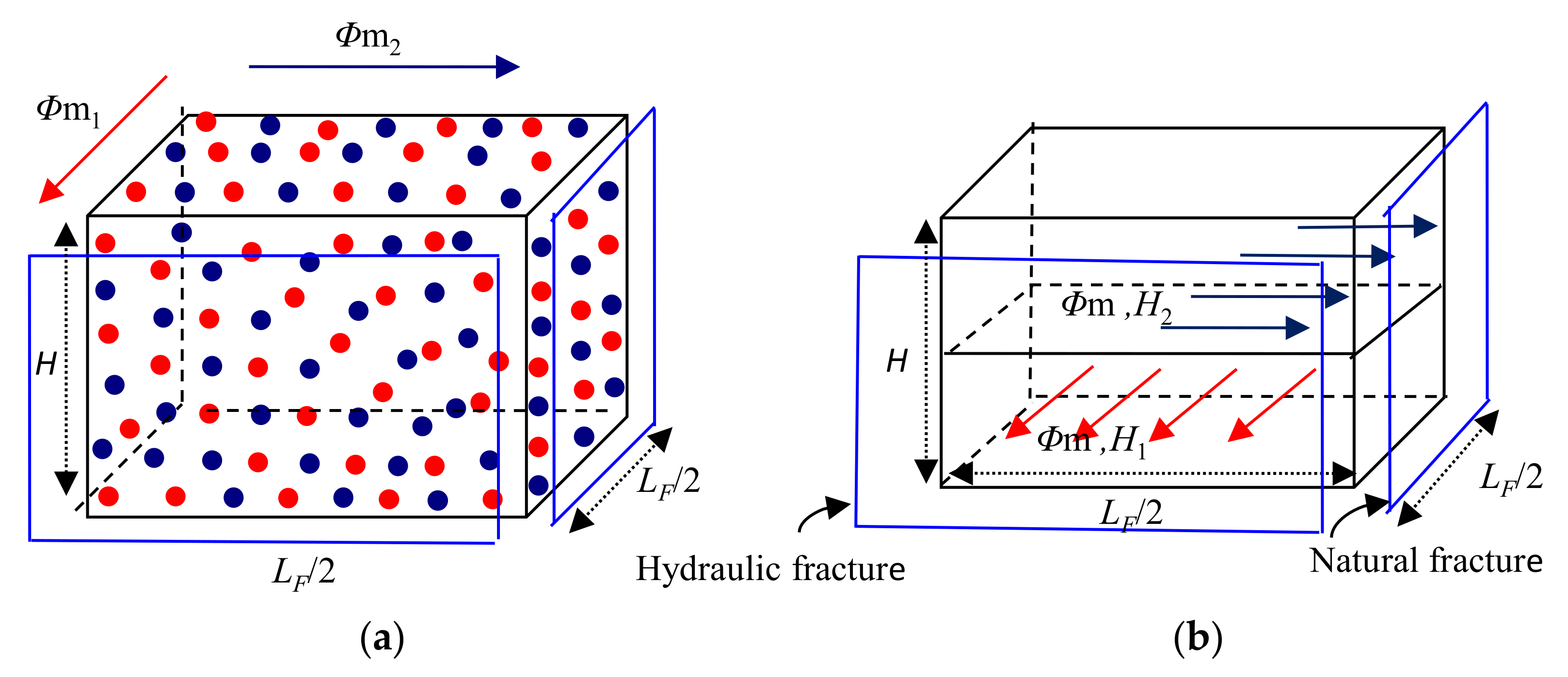
- This paper considers the simultaneous depletion from the matrix into HF and NF. The matrix in SRV region is artificially divided into two distinct segments which are denoted as sub-matrix m1 and sub-matrix m2 respectively. The depletion process from the matrix to HF and NF in SRV region (seen in Figure 1b);
- Sub-matrix m1 feeds the HF via inter-porosity exchange;
- Sub-matrix m2 feeds the NF via inter-porosity exchange.
2.1. Conceptual Model
2.1.1. Conceptual Model 1
- Sub-matrix m1 and sub-matrix m2 mix up with each other evenly, which means that both of them have the same width Lf, length LF and thickness H (see the Figure 2a);
- Sub-matrix m1 and sub-matrix m2 have different porosities denoted as Φm1 and Φm2, and the total porosity of the total matrix denoted as Φm is the sum, presented as:
2.1.2. Conceptual Model 2
- Sub-matrix m1 and sub-matrix m2 are strictly separated in the vertical direction, and the whole matrix is divided into two layers.
- Sub-matrix m1 and sub-matrix m2 have different thicknesses denoted as H1 and H2, and the total thickness of the matrix is denoted as H, which is the sum of those two parts:
2.2. Mathematical Model
2.2.1. Conceptual Model 1
- The pressure equation governing fluid flow in hydraulic fracture is given as:
- The pressure equation governing fluid flow in natural fracture is given as:
- The pressure equation governing fluid flow in matrix 1 is given as:
- The pressure equation governing fluid flow in matrix 2 is given as:
2.2.2. Conceptual Model 2
- The pressure equation governing fluid flow in hydraulic fracture is given as:
- The pressure equation governing fluid flow in natural fracture is given as:
- The pressure equation governing fluid flow in matrix 2 is given as:In the lower layer unit, the mathematical model is described by the following differential equations.
- The pressure equation governing fluid flow in hydraulic fracture is given as:
- The pressure equation governing fluid flow in natural fracture is given as:
- The pressure equation governing fluid flow in matrix 1 is given as:
2.3. Model Solution
3. Results and Discussion
3.1. Model Validation
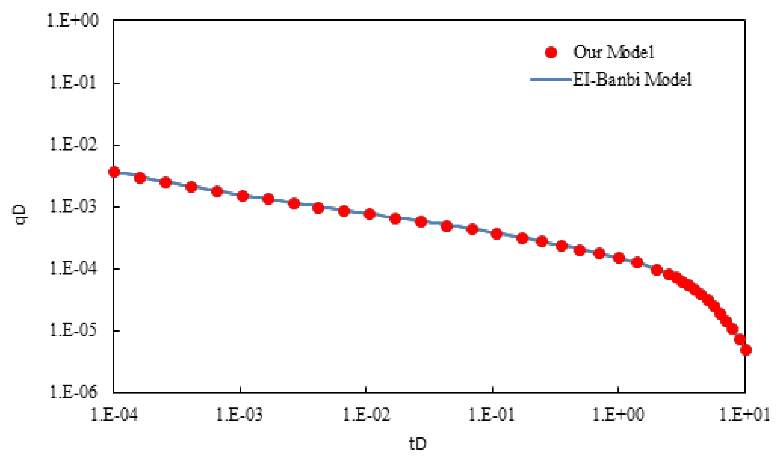
3.1.1. Validation with Analytical Approach
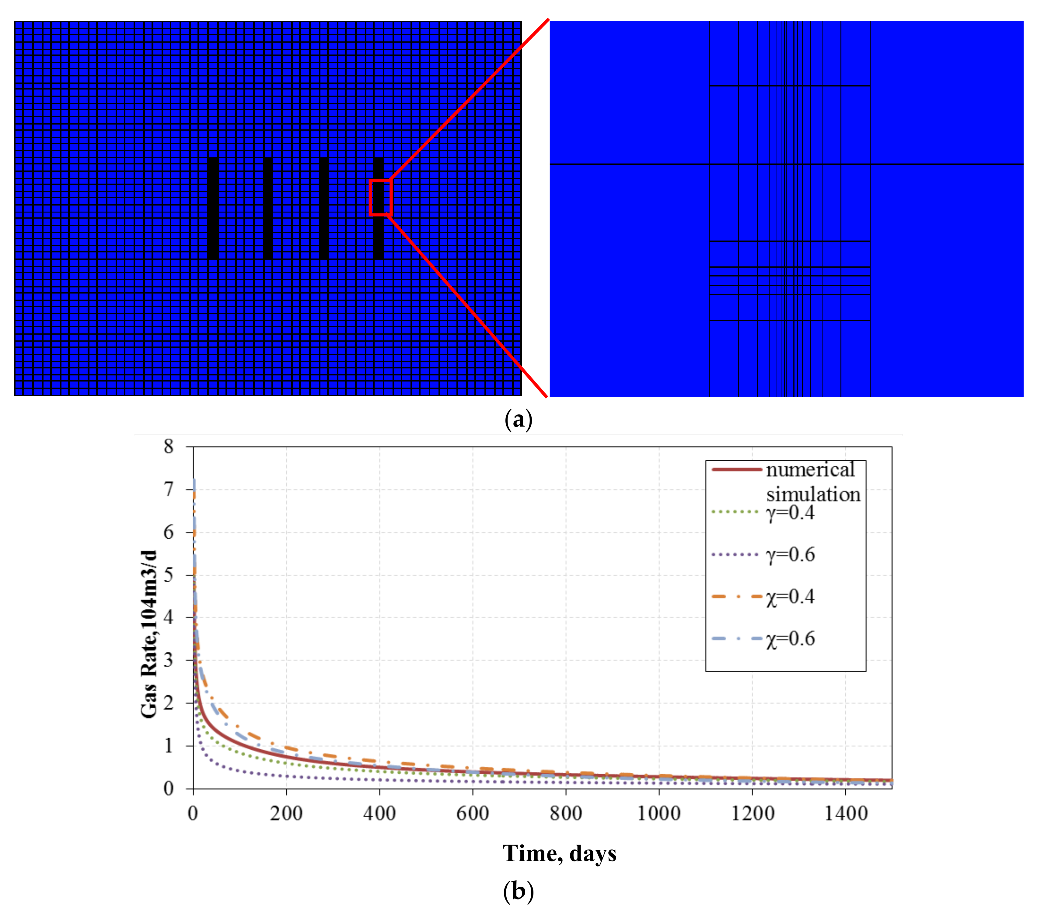
3.1.2. Validation with Numerical Approach
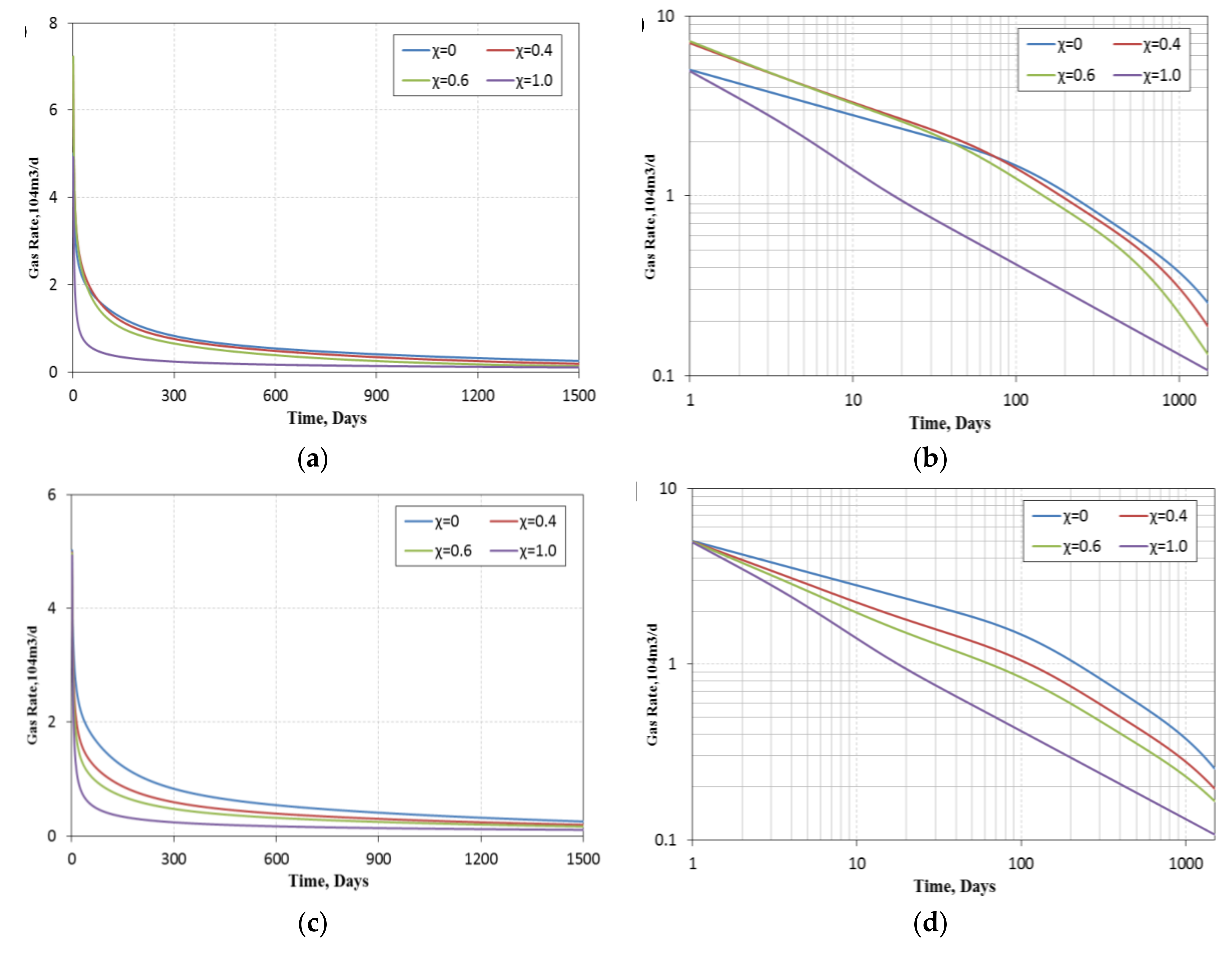
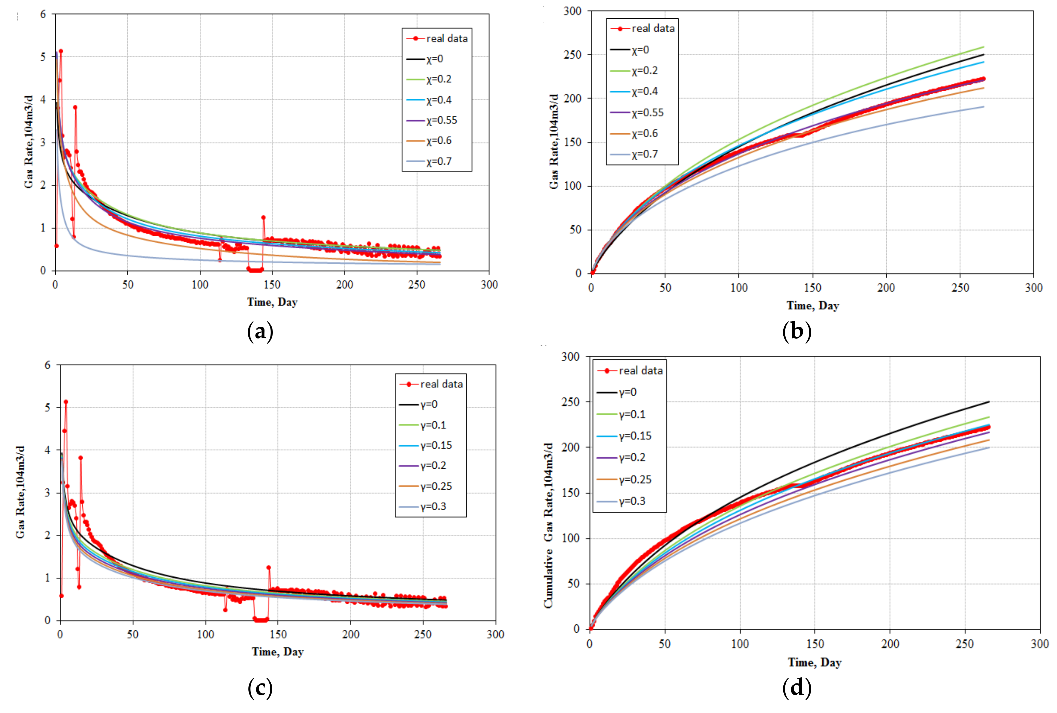
3.2. Sensitivity Analysis
4. Model Aggregation
4.1. GLUE Method
4.2. Application Illustration
4.2.1. Procedure
- Actual production data are matched based on model 1 and model 2 respectively. As a result, the most reliable value of pore volume ratio χ and thickness ratio γ can be obtained;
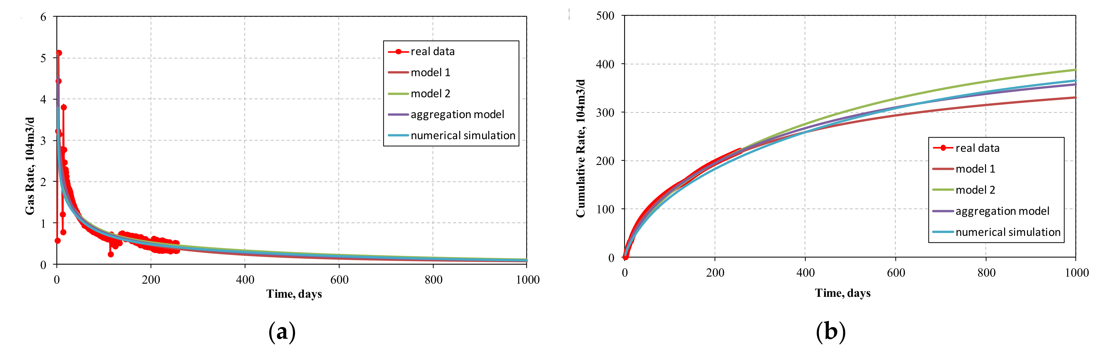
- Based on history and predicted curves, the likelihoods can be calculated respectively for model 1 and model 2 using Equation (18), and then the likelihoods can be normalized using Equation (19);
- Based on Equation (20), we can calculate the production rate and cumulative rate at a certain production time T0, and then compare those results with the numerical simulation by calculating standard deviation using Equation (21).
4.2.2. Field Example
5. Conclusions
Author Contributions
Acknowledgments
Conflicts of Interest
Appendix A. Details on Mathematical Model
Appendix A.1. Conceptual Model 1
- For hydraulic fracture: diffusivity equation that control HF-horizontal well communication is described as
- For Natural fracture: diffusivity equation that control NF-HF communication is described as
- For sub-matrix 1: diffusivity equation that control matrix-HF communication is described as
- For sub-matrix 2: diffusivity equation that control matrix-NF communication is described as
Appendix A.2. Conceptual Model 2
Appendix A.3. Initial and Boundary Condition
- In model 1, inner boundary conditions are given as:
- In model 2, inner boundary condition in HF, NF and matrix are given as:
- In model 1 and model 2, outer boundary conditions in HF, NF and matrix are given as:
Appendix B. Constant Pressure Solution
Appendix B.1. Dimensionless Model in Laplace Domain
Appendix B.1.1. Model 1
Appendix B.1.2. Model 2
Appendix B.2. Laplace-Domain Solution
Appendix B.2.1. Model 1
Appendix B.2.2. Model 2
References
- Clarkson, C.R. Production data analysis of unconventional gas wells: Review of the theory and best practices. Int. J. Coal Geol. 2013, 109, 101–149. [Google Scholar] [CrossRef]
- Nobakht, M.; Clarkson, C.R.; Kaviani, D. New type curves for analyzing horizontal well with multiple fractures in shale gas reservoir. J. Natl. Gas Sci. Eng. 2013, 10, 99–112. [Google Scholar] [CrossRef]
- Ozkan, E.; Brown, M.; Raghavan, R.; Kazemi, K.H. Comparison of fractured horizontal well performance in tight sand and shale gas reservoirs. SPE Reserv. Eval. Eng. 2011, 14, 248–259. [Google Scholar] [CrossRef]
- Stalgorova, E.; Mattar, L. Practical model to simulate production of horizontal wells with branch fractures. In Proceedings of the SPE Canadian Unconventional Resource Conference, Calgary, AB, Canada, 30 October–1 November 2012. [Google Scholar]
- Stalgorova, E.; Mattar, L. Analytical model for history matching and forecasting production in multi-fractured composite systems. In Proceedings of the SPE Canadian Unconventional Resource Conference, Calgary, AB, Canada, 30 October–1 November 2012. [Google Scholar]
- Weng, X.; Kressem, O.; Cohen, C.; Wu, R.; Gu, H. Modeling of hydraulic fracture network propagation in a naturally fractured formation. In Proceedings of the SPE Hydraulic Fracturing Conference and Exhibition, The Woodlands, TX, USA, 24–26 January 2011. [Google Scholar]
- Tan, L.; Zuo, L.; Wang, B. Methods of Decline Curve Analysis for Shale Gas Reservoirs. Energies 2018, 11, 552. [Google Scholar] [CrossRef]
- Wu, K.; Olson, J.E. Simultaneous multifracture treatments: Fully coupled fluid flow and fracture mechanics for horizontal wells. SPE J. 2015, 20, 337–346. [Google Scholar] [CrossRef]
- Zuo, L.; Yu, W.; Wu, K. A fractional decline curve analysis model for shale gas reservoirs. Int. J. Coal Geol. 2016, 163, 140–148. [Google Scholar] [CrossRef]
- Li, Y.; Zuo, W.; Yu, W.; Chen, Y. A Fully Three Dimensional Semianalytical Model for Shale Gas Reservoirs with Hydraulic Fractures. Energies 2018, 11, 436. [Google Scholar] [CrossRef]
- Barenblatt, G.I.; Zhelto, I.P.; Kochina, I.N. Bacis Concepts of the theory of Seepage of Homogeneous Liquids in Fissured Rocks. J. Appl. Math. Mech. 1960, 24, 852–864. [Google Scholar] [CrossRef]
- Warren, J.E.; Root, P.J. The Behavior of Naturally Fractured Reservoirs. SPE J. 1963, 3, 245–255. [Google Scholar] [CrossRef]
- Kazemi, H. Pressure Transient of Naturally Fractured Reservoirs with Uniform Fracture Distribution. SPE J. 1969, 12, 451–462. [Google Scholar] [CrossRef]
- De Swaan, O.A. Analytical Solution for Determining Naturally Fractured Reservoir Properties by Well Testing. SPE J. 1976, 12, 117–122. [Google Scholar] [CrossRef]
- Ozkan, E.; Raghavan, R. Some applications of pressure derivative analysis procedure. In Proceedings of the 62nd Annual Technical Conference and Exhibition, Dallas, TX, USA, 27–30 September 1987. [Google Scholar]
- Al-Ghamdi, A.; Ershaghi, I. Pressure Transient Analysis of Dually Fractured Reservoirs. SPE J. 1996, 2, 23–25. [Google Scholar] [CrossRef]
- Liu, J.C.; Bodvarsson, G.S.; Wu, Y.S. Analysis of Flow Behavior in Fractured Lithophysal Reservoirs. J. Contam. Hydrol. 1996, 62–63, 189–211. [Google Scholar] [CrossRef]
- Wu, Y.S.; Liu, H.H.; Bodvarsson, G.S. A Triple-Continuum Approach for Modeling Flow and Transport Process in Fractured Rock. J. Contam. Hydrol. 2004, 73, 145–179. [Google Scholar] [CrossRef] [PubMed]
- Dreier, J. Pressure Transient Analysis of Wells in Reservoirs with a Multiple Fracture Network. Master’s Thesis, Colorado School of Mines, Golden, CO, USA, 2004. [Google Scholar]
- El-Banbi, A.H. Analysis of Tight Gas Wells. Ph.D. Thesis, Texas A&M University, College Station, TX, USA, 1998. [Google Scholar]
- Al-Ghamdi, A.; Chen, B.; Behmanesh, H.; Qanbari, F.; Aguilera, R. An improved triple-porosity model for evaluation of naturally fractured reservoir. SPE Reserv. Eval. Eng. 2011, 8, 397–404. [Google Scholar] [CrossRef]
- Zhao, Y.L.; Zhang, L.H.; Wu, F. Analysis of horizontal well pressure behavior in fractured low permeability reservoirs with consideration of threshold pressure gradient. J. Geophys. Eng. 2013, 10, 1–10. [Google Scholar] [CrossRef]
- Obinna, E.D.; Hassan, D. A model for simultaneous matrix depletion in natural and hydraulic fracture network. J. Natl. Gas Sci. Eng. 2014, 16, 57–69. [Google Scholar]
- Tian, L.; Xiao, C. Well testing model for multi-fractured horizontal well for shale gas reservoir with consideratuon of dual diffusion in matrix. J. Natl. Gas Sci. Eng. 2014, 21, 283–295. [Google Scholar] [CrossRef]
- Stehfest, H. Numerical inversion of Laplace transforms-algorithm 368. Commun. ACM 1970, 13, 47–49. [Google Scholar] [CrossRef]
- Rasheed, O.; Bello, R.; Wattenbarger, A. Rate Transient analysis in naturally fractured shale gas reservoirs. In Proceedings of the CIPC/SPE Gas Technilogy Symposium 2008 Joint Conference, Calgary, AB, Canada, 16–19 June 2008. [Google Scholar]
- Beven, K.J.; Binley, A. The future of Distribution Models: Model Calibration and Uncertainty Prediction. Hydrol. Process 1992, 6, 278–289. [Google Scholar] [CrossRef]


| Dimensionless Variables | Definitions |
|---|---|
| Dimensionless pseudo pressure | , where |
| Dimensionless time | , |
| Dimensionless space | , , |
| Dimensionless inter-porosity index | , , |
| Dimensionless storability ratio | , where |
| Dimensionless conductivity ratio | |
| Dimensionless production data | |
| Dimensionless permeability ratio |
| Condition | Model 1 | Model 2 | |
|---|---|---|---|
| Initial | |||
| Inner boundary | HF | ||
| NF | , | , , | |
| Matrix | , , | , , | |
| Outer boundary | , , | ||
| Parameters | Symbol | Unit | Value |
|---|---|---|---|
| Initial pressure | Pi | MPa | 20 |
| Downhole pressure | Pwf | MPa | 15 |
| Formation temperature | T | K | 333 |
| Horizontal length | L | m | 1200 |
| Formation thickness | H | m | 100 |
| Macro-fracture length | yf | m | 200 |
| Total compressibility of HF | CtF | MPa−1 | 5 × 10⁻⁴ |
| Total compressibility of NF | CtF | MPa−1 | 5 × 10⁻⁴ |
| Total compressibility of Matrix | CtF | MPa−1 | 5 × 10⁻⁴ |
| Porosity of HF | ΦF | Dimensionless | 0.0005 |
| Porosity of NF | Φf | Dimensionless | 0.005 |
| Total porosity of matrix | Φm | Dimensionless | 0.08 |
| Permeability of HF | kF | D | 2 |
| Permeability of natural fracture | kf | D | 10−6 |
| Permeability of sub-matrix m1 | km1 | D | 10−8 |
| Permeability of sub-matrix m2 | km2 | D | 10−8 |
| Langmuir pressure | PL | MPa | 5 |
| Langmuir volume | VL | sm3/m3 | 5 |
| Parameters | Symbol | Unit | Value |
|---|---|---|---|
| Initial pressure | Pi | MPa | 22.5 |
| Downhole pressure | Pwf | MPa | 15 |
| Formation temperature | T | K | 314 |
| Horizontal length | L | m | 1450 |
| Formation thickness | H | m | 48.3 |
| Macro-fracture length | yf | m | 214 |
| Total compressibility of HF | CtF | MPa−1 | 5.2 × 10⁻⁴ |
| Total compressibility of NF | CtF | MPa−1 | 5.2 × 10⁻⁴ |
| Total compressibility of Matrix | CtF | MPa−1 | 5.2 × 10⁻⁴ |
| Porosity of HF | ΦF | Dimensionless | 4.6 × 10⁻⁴ |
| Porosity of NF | Φf | Dimensionless | 5.3 × 10⁻³ |
| Total porosity of matrix | Φm | Dimensionless | 0.078 |
| Permeability of HF | kF | D | 1.8 |
| Permeability of natural fracture | kf | D | 2.1 × 10⁻⁶ |
| Permeability of sub-matrix m1 | km1 | D | 1.2 × 10⁻⁸ |
| Permeability of sub-matrix m2 | km2 | D | 1.2 × 10⁻⁸ |
| Langmuir pressure | PL | MPa | 5.2 |
| Langmuir volume | VL | sm3/m3 | 5.2 |
© 2018 by the authors. Licensee MDPI, Basel, Switzerland. This article is an open access article distributed under the terms and conditions of the Creative Commons Attribution (CC BY) license (http://creativecommons.org/licenses/by/4.0/).
Share and Cite
Cao, M.; Dai, Y.; Zhao, L.; Jia, Y.; Jia, Y. Hybrid Coupled Multifracture and Multicontinuum Models for Shale Gas Simulation by Use of Semi-Analytical Approach. Energies 2018, 11, 1308. https://doi.org/10.3390/en11051308
Cao M, Dai Y, Zhao L, Jia Y, Jia Y. Hybrid Coupled Multifracture and Multicontinuum Models for Shale Gas Simulation by Use of Semi-Analytical Approach. Energies. 2018; 11(5):1308. https://doi.org/10.3390/en11051308
Chicago/Turabian StyleCao, Maojun, Yu Dai, Ling Zhao, Yuele Jia, and Yueru Jia. 2018. "Hybrid Coupled Multifracture and Multicontinuum Models for Shale Gas Simulation by Use of Semi-Analytical Approach" Energies 11, no. 5: 1308. https://doi.org/10.3390/en11051308
APA StyleCao, M., Dai, Y., Zhao, L., Jia, Y., & Jia, Y. (2018). Hybrid Coupled Multifracture and Multicontinuum Models for Shale Gas Simulation by Use of Semi-Analytical Approach. Energies, 11(5), 1308. https://doi.org/10.3390/en11051308