1. Introduction
Electricity is one of the most important sources of energy on earth. Typical approaches use single-stage or single models to forecast electricity sales. In general, single models use two kinds of forecasting techniques: statistical modeling and soft computing modeling. For example, the impacts of population and weather-sensitive parameters on electricity consumption in Delhi were investigated [
1]. Different multiple linear regression models were developed for the various seasons. The residential demand for electricity in Taiwan from 1955 to 1996 was investigated [
2]. In [
2], it was assumed that the electricity demand was a function of population growth, electricity prices, the degree of urbanization, and household disposable income. Different long-term regression models for the prediction of electricity consumption in Italy have been proposed [
3]. The explanatory variables included gross domestic product (GDP), GDP per capita, and population. Additionally, selected economic and demographic variables that affect annual electricity consumption in New Zealand were studied [
4]. Forecasting models that use multiple linear regression analysis have been proposed. The regression model, a Holt-Winters exponential smoothing method, and the trigonometric gray model with a rolling mechanism were proposed to forecast electricity consumption in Romania [
5].
However, regression analysis has its own limitations, such as variation homogeneity for the regression models. Consequently, autoregressive integrated moving average (ARIMA) modeling has been used to forecast electricity sales. ARIMA modeling is appropriate because seasonal effects are included in the forecasts. ARIMA is a well-known forecasting technique that consists of different types of processes. Those processes include autoregressive (AR), moving average (MA), and combined AR and MA. Electricity demand load was forecasted using ARIMA modeling [
6]. Comparisons between ARIMA, seasonal ARIMA, and a regression model for forecasting electricity demand have been conducted [
7]. The forecasting of electric prices was performed using ARIMA [
8]. A combined AR and a finite impulse response filter were proposed for forecasting electricity demand in Lebanon [
9]. Several linear or ARIMA-like models and nonlinear models were studied for forecasting electricity consumption in Taiwan [
10]. Although ARIMA modeling is widely used for forecasting electricity demand or sales, the linear form of ARIMA models may have difficulty capturing the nonlinear pattern of electricity sales data [
11,
12,
13].
In contrast to statistical modeling, the artificial neural network (ANN) and multivariate adaptive regression splines (MARS) techniques contain fewer a priori assumptions. ANN and MARS can also serve as alternative modeling schemes for electricity sales forecasting since both can model nonlinearity and provide good forecasting characteristics [
14,
15,
16,
17,
18]. Determining Turkey’s electricity consumption using ANN training algorithms has been proposed [
19]. A methodology based on ANN was studied to forecast day-ahead electricity spikes and prices in Ontario, Canada [
20]. Three techniques for forecasting electricity consumption (regression analysis, decision trees, and ANN) were investigated [
21]. Least squares support vector machines were used to forecast electricity consumption in Turkey [
22]. Traditional regression analysis and ANN have also been used for comparison purposes; gross electricity generation, installed capacity, total subscribership, and population were used as explanatory variables. ANN and regression analyses were used to forecast energy consumption in Turkey based on socio-economic and demographic variables [
23]. The ANN with four explanatory variables (GDP, population, and the amount of imports and exports) was considered to be the most suitable model. ANN, linear regression, and nonlinear regression approaches were considered in forecasting the electricity consumption of residential and industrial sectors in Turkey [
24]. The explanatory variables for the models included installed capacity, gross electricity generation, population, and the total number of customers. However, ANN has been criticized for its long training process when designing the optimal structure [
25,
26].
In recent years, hybrid forecasting models with feature selection techniques (FSTs) have been studied for electricity sales forecasting. A hybrid model with fast ensemble empirical mode decomposition, variational mode decomposition, and ANN was investigated in forecasting electricity prices [
27]. A hybrid forecasting approach for managing and scheduling electric power generation has also been studied [
28]. A combined model, including wavelet transforms, ARIMA, and ANN, was used to simultaneously forecast electricity demand and price [
29]. A hybrid approach that integrated wavelet transforms, a kernel extreme learning machine, and an autoregressive moving average was developed to forecast electricity prices [
30]. A combined forecasting approach based on ANN, an adaptive network-based fuzzy inference system, and seasonal ARIMA was proposed to forecast short-term electricity demand [
31]. A hybrid forecasting model that combined a support vector machine and ARIMA with external input modules was proposed to forecast mid-term electricity market clearing prices [
32]. In [
32], it was assumed that all forecasting input data were given, which may not be practical.
The work used a tree-based machine learning technique to predict the electricity price [
33]. Additionally, the hybridization of ARIMA and soft computing techniques to enhance the accuracy of food crop price prediction was incorporated in the design [
34,
35]. Additionally, they employed an ARIMA approach to predict conventional electrical load and charging demand of electric vehicles [
36]. The study improved the accuracy of ARIMA forecaster by optimizing the integrated and AR order parameters. In [
37], they considered the users’ long-term electricity load scheduling problem and model the changes of the price information and load demand as a Markov decision process. This study developed an online load scheduling learning algorithm based on the actor-critic method to determine the users’ Markov perfect equilibrium policy.
After the literature review for electricity sales and demand forecasting was completed in this study, we made the following observations. The first and most important observation was that the forecasting of electricity sales is extremely worthy of investigation. The second observation was that a significant number of forecasting models generate forecasts based on certain known explanatory variables, which may not be feasible in practical applications. The third observation was that traditional approaches, such as regression, econometric, and ARIMA, as well as soft computing techniques, are widely used for electricity sales forecasting [
38]. However, a good technique, MARS, has not been adopted for electricity sales forecasting. The final observation is that electricity sales data series may possess linear and/or nonlinear features and that hybrid forecasting techniques should be used to improve forecasting accuracy. However, although most FSTs in hybrid models can provide a good selection of significant explanatory variables, these variables may not be available in the future and those significant explanatory variables may thus not be appropriate for electricity sales forecasting.
This study proposed the single ANN, single MARS, hybrid ARIMA and ANN (ARIMA-ANN), and hybrid ARIMA and MARS (ARIMA-MARS) models to forecast the industrial electricity, residential electricity, and commercial electricity sales (IERECES) in Taiwan without using any explanatory variables. The reason for using ANN is that it is one of the most widely used soft computing methods for electricity sales forecasting. The reason for using MARS is that it has not been used for electricity sales forecasting. Additionally, both the ANN and MARS techniques are suitable for modeling the nonlinear features of electricity sales data series. Finally, the reason for using the hybrid ARIMA-ANN and ARIMA-MARS is that they possess linear and nonlinear forecasting abilities. The fundamental concept of the hybrid forecasting scheme is to capture various characteristics in the data by making use of individual model’s dominance [
39,
40]. Therefore, the hybrid technique can improve forecasting accuracy using each model’s unique features. Since single ANN and MARS were used to forecast the IERECES in Taiwan, this study integrated ARIMA and ANN, and ARIMA and MARS as the hybrid models. Most importantly, since most FSTs select important explanatory variables that may not be available in the future, this study logically employed ARIMA modeling as the FST for the proposed hybrid forecasting models. ARIMA can identify significant self-predictor variables that will be available in the future. In this study, a self-predictor variable refers to the future values of the variable that can be computed using the preceding or available values of the variable itself.
The real dataset of IERECES in Taiwan was collected from January 2006 to July 2016. The IERECES dataset contains three monthly data series: industrial electricity (IE), residential electricity (RE), and the commercial electricity (CE) sales series. This study used the first 115 monthly data records to build different forecasting models and used the last 12 monthly data records for confirmation. The rest of this paper is structured as follows.
Section 2 presents the design of different forecasting methodologies.
Section 3 introduces the real IERECES data series in Taiwan. Three types of electricity sales series are fitted to four single and two hybrid forecasting models, without using any explanatory variables.
Section 4 provides the discussion about forecasting comparisons for four single models and two hybrid models. The final section addresses the research findings and conclusions inferred from this study.
2. Materials and Methods
In this section, the concept and the modeling processes for ARIMA, ANN and MARS are briefly introduced.
2.1. Autoregressive Integrated Moving Average (ARIMA) Modeling
A time series consists of a set of observations on the values that a variable takes at different times, ordered sequentially. Because seasonal effects are involved in electricity sales forecasting, time series forecasting techniques should be used. A well-known ARIMA forecasting technique was developed to predict time series data [
41]. A general seasonal ARIMA model is described as follows [
41]:
where
| B: | the backward shift operator, defined as: , |
| L: | the number of seasons in a year, and L = 12 for monthly data, |
| d: | the values of non-seasonal difference transformations, |
| D: | the values of seasonal difference transformations, |
| Zt: | the working series, which are stationary after fitting a suitable difference transformation from original time series Yt |
| δ: | an unknown constant, |
| at: | white noise at time t, which is independent and identical (iid) with normal distribution, |
| p: | the order of non-seasonal autoregressive (AR) models, |
| P: | the order of seasonal AR models, |
| q: | the order of non-seasonal moving average (MA) models, |
| Q: | the order of seasonal MA models, |
| a polynomial function for a non-seasonal AR model, defined as: , |
| a polynomial function for a seasonal AR model, defined as: , |
| a polynomial function for a non-seasonal MA model, defined as: , |
| a polynomial function for a seasonal MA model, defined as: , |
The original nonstationary time series should be transformed into a stationary working series by differencing. Typically, the transformation is carried out using four sets of d and D. Those four sets include (d, D) = (0, 0), (d, D) = (1, 0), (d, D) = (0, 1), and (d, D) = (1, 1). After obtaining stationary working series, we can apply the sample autocorrelation function (ACF) and sample partial autocorrelation function (PACF) to determine the values of p, P, q, and Q for the seasonal ARIMA models.
Additionally, diagnostic checks for testing the lack of fit of a time series model must be performed. The Ljung–Box test was applied to the residuals of a time series after fitting a seasonal ARIMA model to the working series [
42]. Instead of testing randomness at each distinct lag, the Ljung–Box statistic was used to test the overall randomness based on several lags. The Ljung–Box statistic is described as follows:
where
- Q:
Ljung–Box statistics, and the asymptotic distribution of Q follows a chi-square distribution with k-np degrees of freedom,
- np:
number of parameters other than that must be estimated in the ARIMA model under consideration,
- n:
the number of observations,
- :
the square of the sample autocorrelation of the residuals at lag l.
The Ljung–Box test rejects the null hypothesis, which indicates that the underlying model has significant lack of fit if:
where
is the chi-square distribution table value with
k-
np degrees of freedom and significance level α.
2.2. Artificial Neural Network (ANN) Modeling
An ANN is a massively parallel system composed of highly interconnected and interacting processing units that are based on neurobiological models. ANNs handle information via the interactions of neurons [
43]. ANNs have been extensively used in modeling nonlinear processes because of their associated memory characteristics and generalization capabilities. In this study, an ANN was used as an alternative to the single modeling approach to forecast IERECES data series in Taiwan.
The input, hidden, and output layers consist of the ANN. Those three layers contain several nodes or neurons connected by links. An ANN contains nodes that are connected to themselves, which enables a node to influence other nodes and itself. An external source provides input signals to the nodes in the input layer, and the output signals are produced by the nodes in the output layer. The hidden nodes are nonlinear functions of the input variables. The predicted output variable is a function of the nodes in the hidden layer.
ANN modeling can be simply described as follows. For an ANN model, the relationship between inputs (
x1,
x2, …,
xa) and output (
y) is represented as [
16]
where
and
are the connection weights of the model;
a denotes the number of input nodes;
b stands for the number of hidden nodes; and
denotes the error term. In the hidden layer, the transfer function is often used with a logistic function [
16]:
Consequently, the ANN transports nonlinear functional mapping from the inputs (
I1,
I2, …,
Ia) to the output
O; namely, [
16]
where
w is a vector of parameters and
f is a function determined by the ANN structure and the connection weights.
2.3. Multivariate Adaptive Regression Splines (MARS) Modeling
MARS was initially developed as a procedure that modeled the relationships between a few variables [
44]. The modeling procedure for MARS is based on a divide-and-conquer strategy where training sets are partitioned into separate regions. Those regions are determined by the regression equation. MARS can usually reveal the important data characteristics that often hide in high-dimensional data series. It designs the models by fitting piecewise linear regressions, and the nonlinearity of a model is approximated by using separate regression slopes at distinct intervals in the explanatory variable space. Therefore, the slope of the regression line changes from one interval to the next as the two “knot” points are crossed. The variables and endpoints of the intervals for each variable can be obtained via a fast but intensive search procedure.
The general MARS model can be described as follows [
25]:
where
b0 and
bm are the parameters,
M is the number of basis functions (BFs),
Jm is the number of knots,
Sjm takes on values of either 1 or −1 and shows the right or left sense of the corresponding step function,
is the label of the independent variable, and
ljm is the knot location. The optimal MARS model is selected in a two-step procedure. The first step is to build many BFs to initially fit the data. The BFs are deleted in the order of least contributions to most contributions using the generalized cross-validation (GCV) criterion in the second step. When a variable is removed from the model, the measure of variable importance is provided by computing the GCV values. The GCV is described as follows [
25]:
where
N is the number of observations and
C(M) is the set of cost penalty measures of a model containing
M BFs.
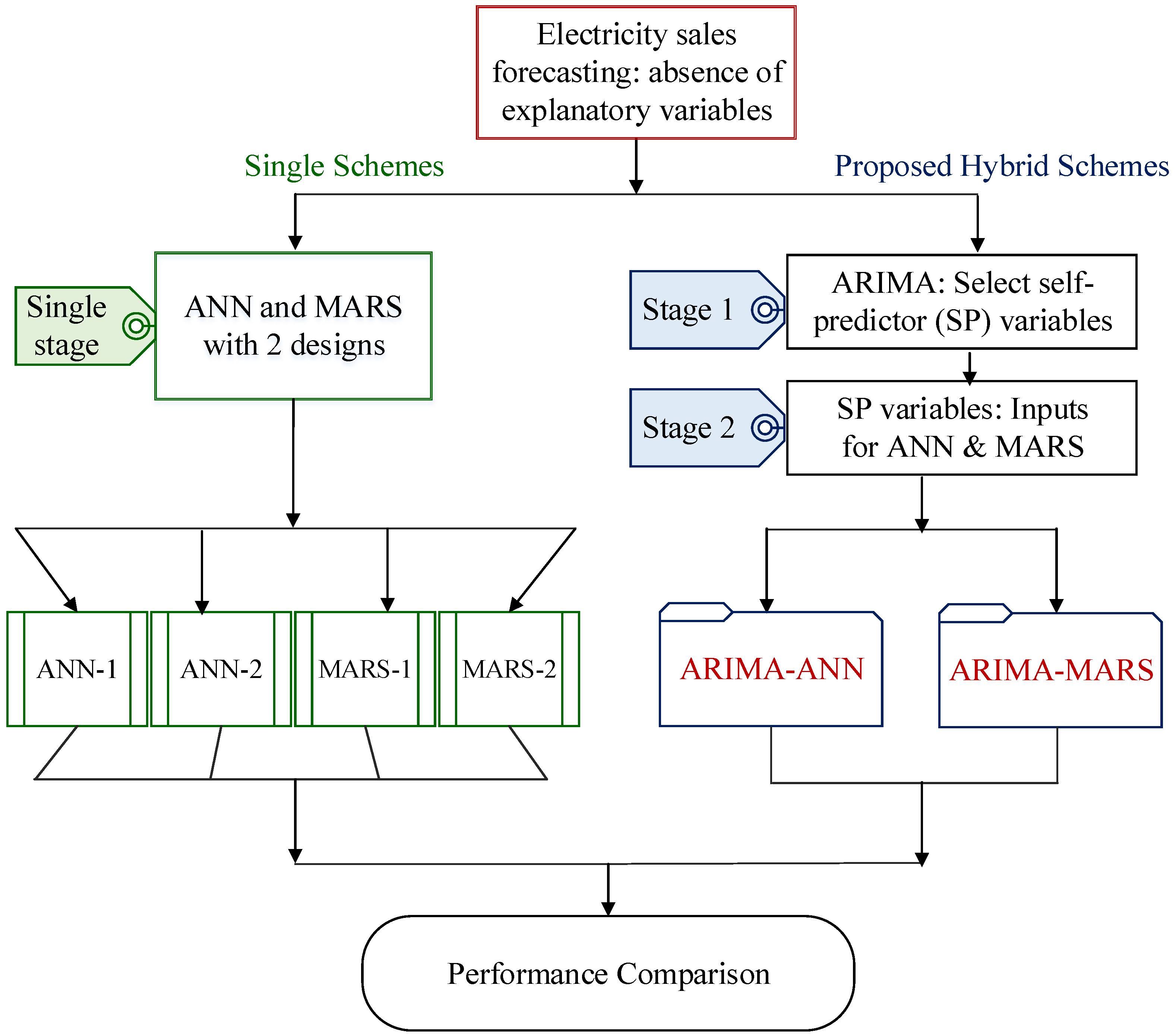
2.4. Research Framework
Figure 1 shows a generalized depiction of the research framework. As shown in
Figure 1, since no explanatory variables were used to forecast the electricity sales in this study, we proposed two types of schemes for ANN and MARS modeling.
The first (single) scheme contains two designs. In ANN modeling, the first design arbitrarily selects the preceding two observations at time t-1 and t-2 (i.e., yt-1 and yt-2) to serve as the self-predictor variables. Thus, the two variables yt-1 and yt-2 are considered as two input variables and the variable yt is deemed the output variable. Since seasonal effects may influence IERECES forecasts, the second ANN design in this study used the preceding 12 observations to forecast electricity sales at time t, and the second design used 12 variables, yt-1, yt-2, yt-3, …, and yt-12, to serve as input variables and used the single variable yt to serve as the output for ANN modeling; that is, the second design used 12 input nodes and one output node for the ANN structure. The first and the second designs of ANN are denoted as ANN-1 and ANN-2, respectively. In the modeling of MARS, this study also used the same input structure as ANN modeling, that is, it used two designs for the input variables of MARS modeling. The first design used yt-1 and yt-2 as two input variables and yt as the output variable. The second design considered 12 variables, yt-1, yt-2, yt-3, …, and yt-12 as the input variables and yt as the output variable. The first and the second designs of MARS are denoted as MARS-1 and MARS-2, respectively.
The second (proposed hybrid) scheme included the hybridization of ARIMA and ANN (i.e., ARIMA-ANN) and ARIMA and MARS (i.e., ARIMA-MARS). For the proposed hybrid modeling, this study incorporated FSTs with ANN and MARS to develop forecasting models. The proposed hybrid modeling used the ARIMA as an FST to extract significant self-predictor variables in the first stage. In the second stage, the selected significant self-predictor variables are then served as the inputs for the ANN and MARS forecasting models. Finally, the performance comparison between the single stage models and the proposed hybrid models is discussed.
3. Results
3.1. Datasets and Performance Criteria
Three types of electricity sales data were provided by the Taiwan Power Company to verify the effectiveness of the proposed hybrid modeling. These three datasets covered IERECES from January 2006 to July 2016. The datasets consisted of 127 records for each type of electricity sales. Among them, 115 data records were used to develop the different forecasting models, and the remaining 12 data records were used to perform model confirmation.
In this study, we use the mean absolute percentage error (MAPE), root mean square error (RMSE), and mean absolute difference (MAD) to measure the prediction capability of the models. These prediction measurements are defined as follows [
26]:
where
et is the value of the residual at time
t.
MAPE, MAD, and RMSE are measures of the deviation between actual and forecasted values. These measurements can also be used to evaluate forecasting error. The lower the MAPE, MAD, and RMSE values, the closer the forecasted values were to the actual values. Notice that the MAPE metric may be considered to be biased, being relevant only when there are no extreme values in the data sets (including zeros). In this study, since the values of electricity sales are not zeros or near-zeros, MAPE metric can provide a meaningful performance measure.
Additionally, in here, the ANN models were constructed using Qnet97 simulator, which was designed by Vesta Services Inc. (Tampa, FL, USA). For MARS modeling, the package “MARS”, which was developed by Salford Systems, was employed in this study.
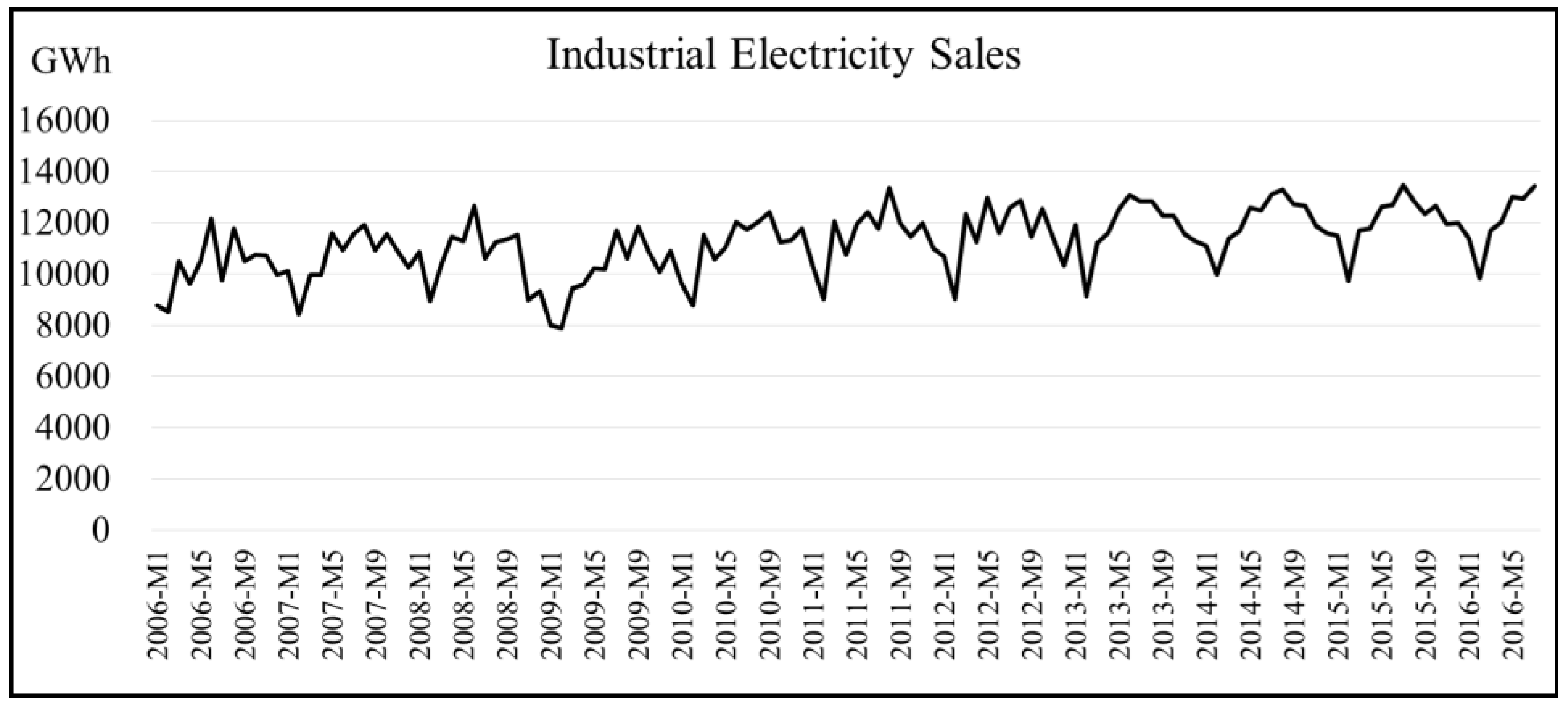
3.2. Forecasting Results for Industrial Electricity (IE) Sales
Figure 2 displays the original time plot for industrial electricity (IE) sales data in Taiwan. After performing ARIMA modeling by using an SAS package (SAS Institute Inc., Cary, NC, USA), this study obtained the parameter estimates reported in
Table 1. Column 2 in
Table 1 indicates that the estimates of the model parameters are 0.62838, −0.94744, and −0.50233. All three values are significantly different from 0 because the corresponding p-values or the “Approx Pr > |t|” values (i.e., Column 5) are all greater than or equal to the type I error, 0.05. Additionally, since the corresponding p-values for the Ljung-Box test are all greater than or equal to 0.05, the conclusion on the appropriateness of the ARIMA model is drawn that the underlying model described in Equation (11) is appropriate for modeling IE sales in Taiwan.
where
It has been stated that more than 75% of neural network applications use the back-propagation neural network (BPNN) structure [
16]. Therefore, this study used the BPNN in designing the ANN forecasting model. For ANN designs, there is no widely accepted way to determine the number of hidden nodes in the ANN structure. Various experiments and rules of thumb have been reported to determine the number of hidden nodes. Too few hidden nodes confine the network generalization capability, whereas too many hidden nodes may lead to the problem of over-training by the network. Additionally, the term {
ni-nh-no} represents the number of neurons in the input layer, the number of neurons in the hidden layer, and the number of neurons in the output layer, respectively. The setting values of hidden nodes were from (2
i − 2) to (2
i + 2), where
i is the number of input variables. Since the learning rate of 0.01 is a very effective setting [
16,
45], this study used the learning rate value of 0.01 for ANN modeling. Moreover, since MAPE is one of the most important performance measurements of forecasting capability, the smallest MAPE was used as the criterion for selecting the ANN topology.
For the ANN model developed herein, two and twelve input nodes were used for the first and second designs, respectively. The hidden nodes were chosen as 2, 3, 4, 5, and 6 for the first design and 22, 23, 24, 25, and 26 for the second design. In this study, when developing the ANN approach, we used the training algorithms of Levenberg-Marquardt which provided the best forecasting accuracy.
After performing the ANN modeling process, the ANN-1 design showed that the {2-6-1} structure provided the best results and the minimum testing MAPE for IE sales. For the ANN-2 design, the best structure for IE sales was {12-25-1}.
Table 2 lists the corresponding MAPE values for different settings of the ANN topologies for the two designs.
For MARS-1 modeling, the input variables and BFs should initially be selected. The variable selection results and the BFs after modeling IE sales data with MARS are summarized in
Table 3. It was observed that the two input variables
yt-1 and
yt-2 played crucial roles in building the MARS forecasting models for forecasting IE data. Accordingly, the MARS forecasting function for IE sales is expressed as follows:
By observing the MARS forecasting function and BF in Equation (12) and
Table 3, we find that BF1 has a positive effect on
yt since the coefficient of BF1 is 0.7271. Therefore, according to the equation of BF1, it can be expected that
yt will increase when the
yt-1 value is higher than the knot point (11261.5). In contrast,
yt-1 will give no information about
yt if
yt-1 stands for lower than the knot point. Additionally,
Table 3 shows that
yt-2 has a negative influence on
yt. The knot point for
yt-2 is 12076.5.
For MARS-2 modeling, the variable selection results and BFs after modeling IE sales data with MARS are summarized in
Table 4. The MARS forecasting function for the IE sales is described as follows:
The proposed hybrid model used the ARIMA as an FST to extract significant self-predictor variables, which served as the inputs for the ANN and MARS models. Based on Equation (11), the ARIMA model indicated that Zt-1, Zt-2, and at-12 would influence Zt. Since at-12 = Zt-12 − Z^t-12, where Z^t-12 is the forecast at time t-12, we observed that Zt-12 would influence Zt. Accordingly, we selected Zt-1, Zt-2, and Zt-12 to serve as the self-predictor variables for the proposed hybrid modeling on IE data series.
The hybrid ARIMA-ANN design used three input nodes and one output node for the ANN structure. The hidden nodes were chosen as 4, 5, 6, 7, and 8 for this design.
Table 5 reports the corresponding MAPE values for different settings of the ANN topologies. For the combined ARIMA-ANN design, the best structure was {3-4-1} for IE sales.
Because
Zt-1,
Zt-2, and
Zt-12 were chosen as self-predictor variables, the hybrid ARIMA-MARS design also used three input nodes and one output node for the MARS structure. The variable selection results and BFs are summarized in
Table 6. The MARS forecasting function for IE sales is described as follows:
where
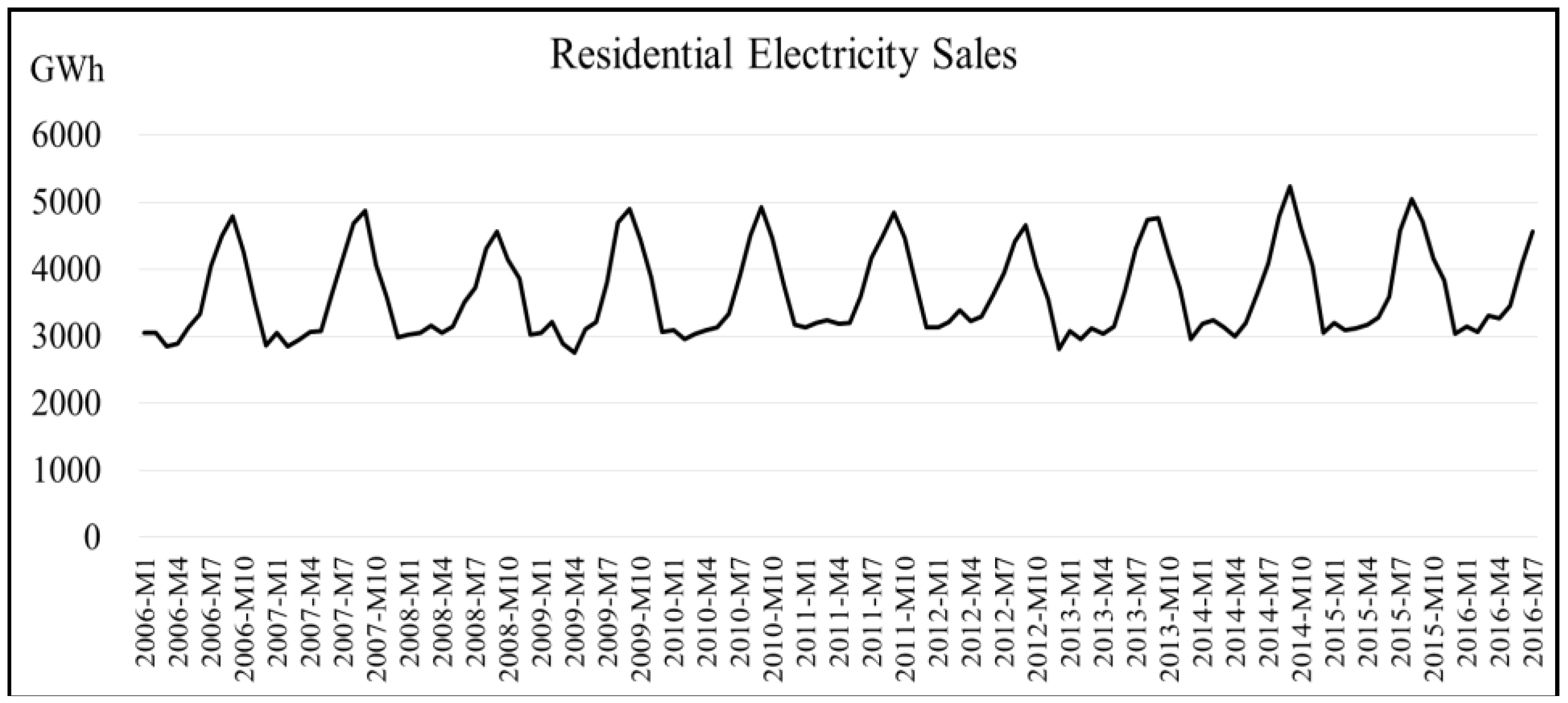
3.3. Forecasting Results for Residential Electricity (RE) Sales
Figure 3 presents the original time plot for RE sales data in Taiwan. The parameter estimates after performing the ARIMA modeling are listed in
Table 7. Column 2 in
Table 7 indicates that the estimates of the model parameters are significantly different from 0. Additionally, since the corresponding p-values for the Ljung-Box test are all greater than or equal to 0.05, the conclusion on the appropriateness of the ARIMA model is drawn that Equation (15) is suitable for modeling the RE sales in Taiwan.
where
This study also used two ANN designs for modeling RE sales, as was the case for the structures for modeling IE sales. The first design used
yt-1 and
yt-2 as the input variables, and the second design used
yt-1,
yt-2,
yt-3, … and
yt-12 as the input variables.
Table 8 presents the corresponding MAPE values for different settings of ANN topologies for the two designs after performing ANN modeling. Observing
Table 8, we notice that the ANN-1 design with {2-2-1} structure had the smallest MAPE for RE sales. For the ANN-2 design, the {12-25-1} structure was associated with the smallest MAPE for RE sales.
For modeling RE sales with MARS, this study used the same two designs. For MARS-1 modeling, the variable selection results and BFs are summarized in
Table 9. The MARS forecasting function for the RE sales is expressed as follows:
For MARS-2 modeling, the variable selection results and the BFs are summarized in
Table 10. Moreover, the MARS forecasting function for the RE sales is described as follows:
For the hybrid modeling for RE sales forecasting, based on Equation (15), ARIMA modeling selected
Zt-1,
Zt-4, and
Zt-12 to serve as the self-predictor variables. Therefore, the hybrid ARIMA-ANN modeling used three input nodes and one output node for the ANN structure. The hidden nodes were chosen as 4, 5, 6, 7, and 8 for this design.
Table 11 lists the corresponding MAPE values for different settings of the ANN topologies. For hybrid ARIMA-ANN modeling, the best structure for RE sales was {3-5-1}.
Additionally, the hybrid ARIMA-MARS design used three input nodes and one output node for the MARS structure. The variable selection results and BFs are summarized in
Table 12. The MARS forecasting function for the IE sales is described as follows:
where
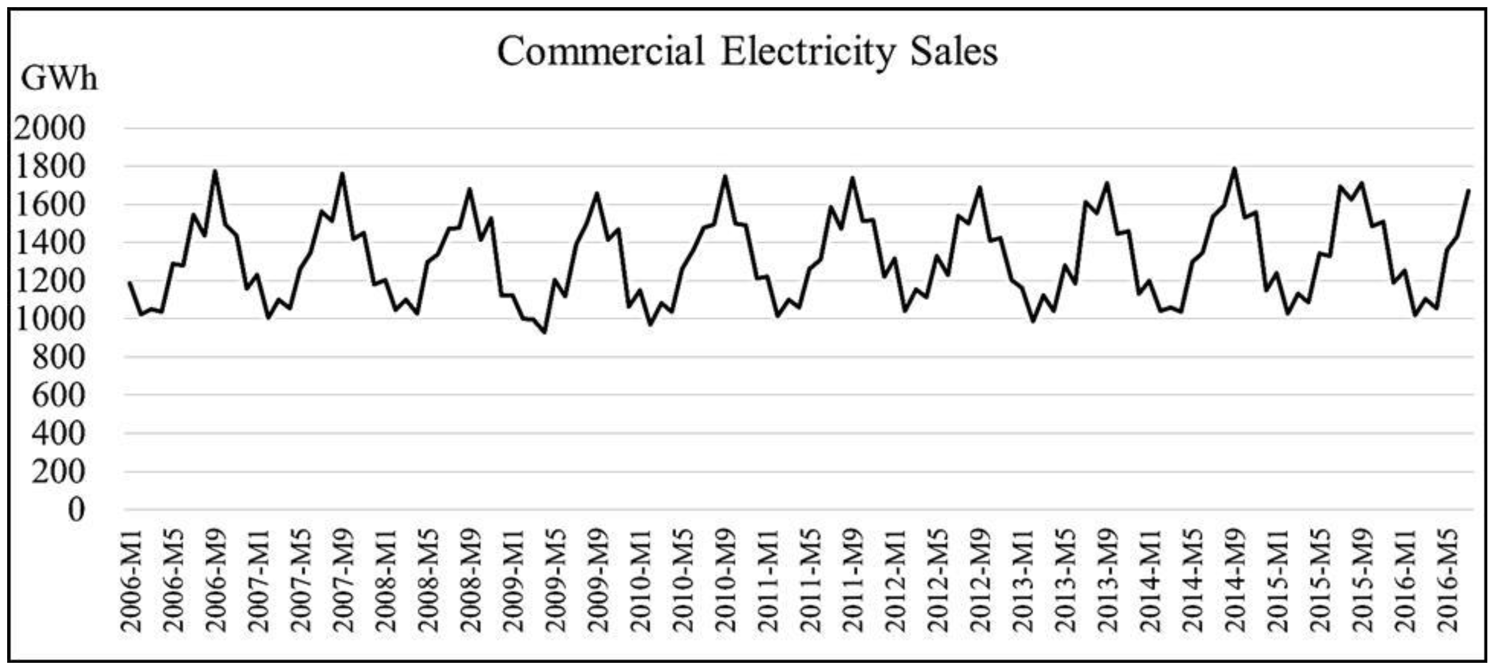
3.4. Forecasting Results for Commercial Electricity (CE) Sales
The original time plot for CE sales data in Taiwan is displayed in
Figure 4.
Table 13 presents the parameter estimates after performing ARIMA modeling. Column 2 in
Table 13 indicates that the estimates of the model parameters are significantly different from 0. Additionally, since the corresponding p-values for the Ljung-Box test are all greater than or equal to 0.05, the conclusion on the appropriateness of the ARIMA model is drawn that Equation (19) is suitable for modeling CE sales in Taiwan.
where
The same two designs for modeling IE and RE sales were applied to the ANN modeling of CE sales. The ANN used three and 12 input nodes for the first and second designs, respectively. After performing ANN modeling,
Table 14 shows the corresponding MAPE values for different settings of the ANN topologies for the two designs. Based on
Table 14, we observed that the ANN-1 design with {2-2-1} structure and ANN-2 design with {12-24-1} structure had the smallest MAPE for CE sales.
In the modeling of MARS for CE sales data, this study also used the same two designs. For MARS-1 modeling,
Table 15 reports the variable selection results and BFs. The MARS forecasting function for the CE sales is described as follows:
For MARS-2 modeling, the variable selection results and BFs are reported in
Table 16. The MARS forecasting function for the CE sales is described as follows:
For the hybrid modeling for CE sales forecasting, we considered
Zt-1,
Zt-2, and
Zt-12 as the self-predictor variables, according to the ARIMA model shown in Equation (19). The hybrid ARIMA-ANN modeling used three input nodes and one output node for the ANN structure. The hidden nodes were chosen as 4, 5, 6, 7, and 8 for this design.
Table 17 lists the corresponding MAPE values for different settings of the ANN topologies. For hybrid ARIMA-ANN modeling, the best structure was {3-5-1} for CE sales.
The hybrid ARIMA-MARS design used three input nodes and one output node for the MARS structure. The variable selection results and BFs are listed in
Table 18. The MARS forecasting function for the CE sales is described as follows:
where
4. Discussion
This study developed various forecasting models to predict three types of electricity sales in Taiwan.
Table 19 shows the forecasting results as well as the MAPE, RMSE, and MAD values of the forecasting models. Low MAPE, RMSE, or MAD values are associated with better forecasting accuracy.
In comparison to the forecasting performance of single models in
Table 19, we observed that the second design exhibited better performance than the first design of the ANN and MARS modeling techniques. The possible reason may be that the second design has more input information than the first design. The results of IERECE sales forecasting also indicate that the second ANN design has better forecasting accuracy than the second MARS design. However, the performance of MARS seems to have been better than the ANN approach for the first design.
As shown in
Table 19, the proposed hybrid models have better forecasting performance than the single models. For example, the proposed hybrid ARIMA-ANN model was associated with MAPE values of 2.21%, 4.51%, and 2.57% for IE, RE, and CE sales forecasting, respectively; these three MAPE values were also the smallest values. Accordingly, our proposed hybrid models provided more accurate results than the single models. For IE sales forecasting, the MAPE percentage improvements (denoted by MAPE
PI) of the proposed ARIMA-ANN model over the two single models ANN-1 and ANN-2 were 169.68% and 29.86%, respectively. The MAPE
PI of ARIMA-ANN over ANN was computed as
For IE sales forecasting, the MAPE
PI of the proposed ARIMA-MARS model over the two single models MARS-1 and MARS-2 were 171.73% and 133.33%, respectively. The MAD and RMSE percentage improvements can be calculated based on Equation (23), and are denoted as MAD
PI and RMSE
PI, respectively.
Table 20 provides a complete comparison of overall improvement percentage. We observed three negative values in
Table 20. For RE sales forecasting, the MAD and RMSE percentage improvements of the ARIMA-ANN over ANN-2 were −3.35% and −17.12%, respectively. For RE sales forecasting, the RMSE percentage improvement of ARIMA-MARS over ANN-1 was −9.83%. A negative percentage improvement means that forecasting performance declined. Nonetheless, the magnitudes of those three negative values are small and only have minor effects on forecasting performance. Additionally, the associated MAPE percentage improvements for those negative values were all positive. That is, if a forecasting model has the minimum MAPE, this does not mean that it has the minimum MAD or RMSE. As shown in
Table 19 and
Table 20, the proposed hybrid models outperform the single models.
Additionally,
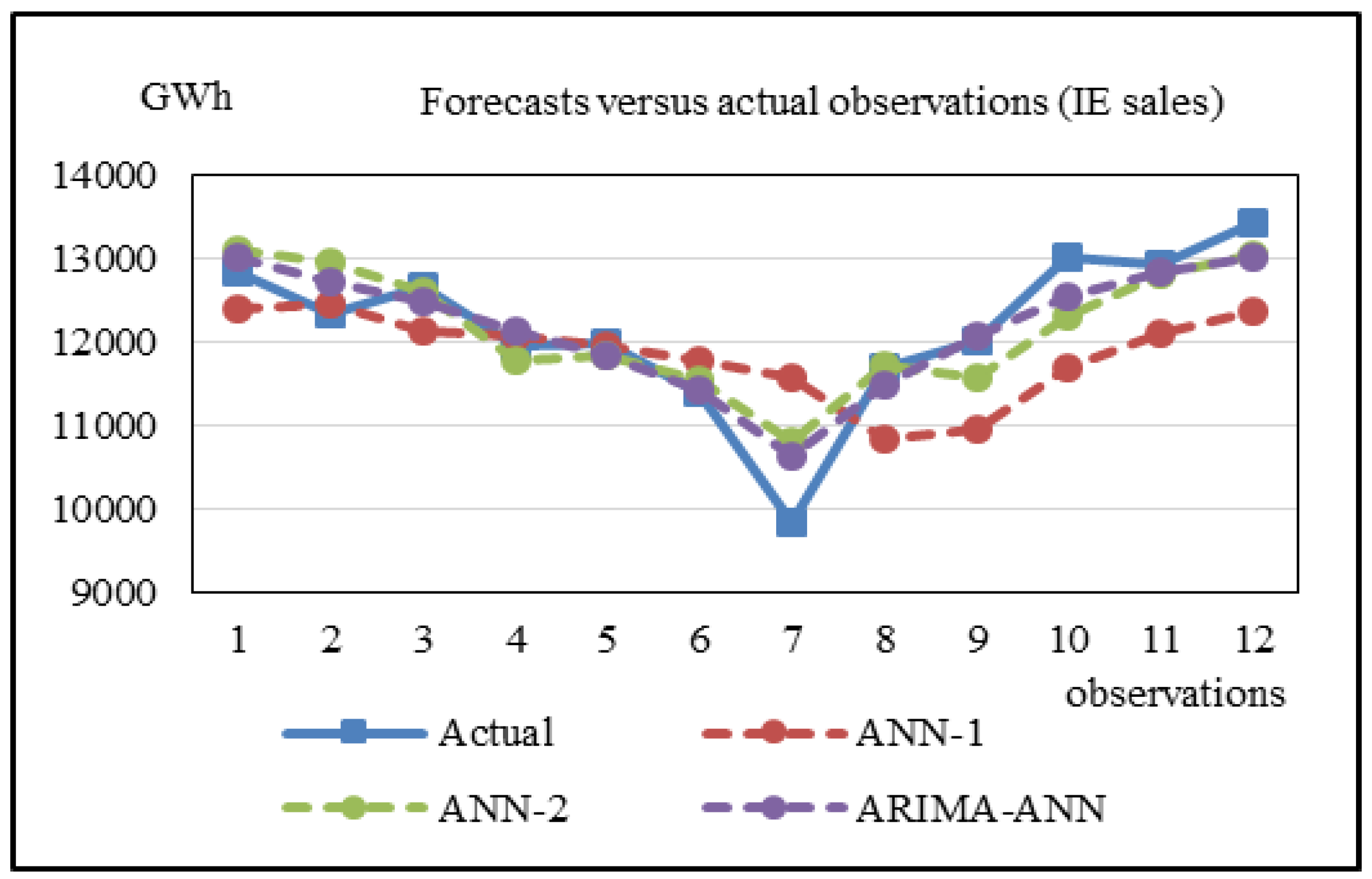
Figure 5 displays the forecasts of IE sales obtained by using ANN-1, ANN-2, and the proposed ARIMA-ANN models for the last twelve testing records. We notice that the forecasts of the ARIMA-ANN model are closer to the actual observations, whereas the forecasts of the ANN-1 model seem far away from the actual observations.
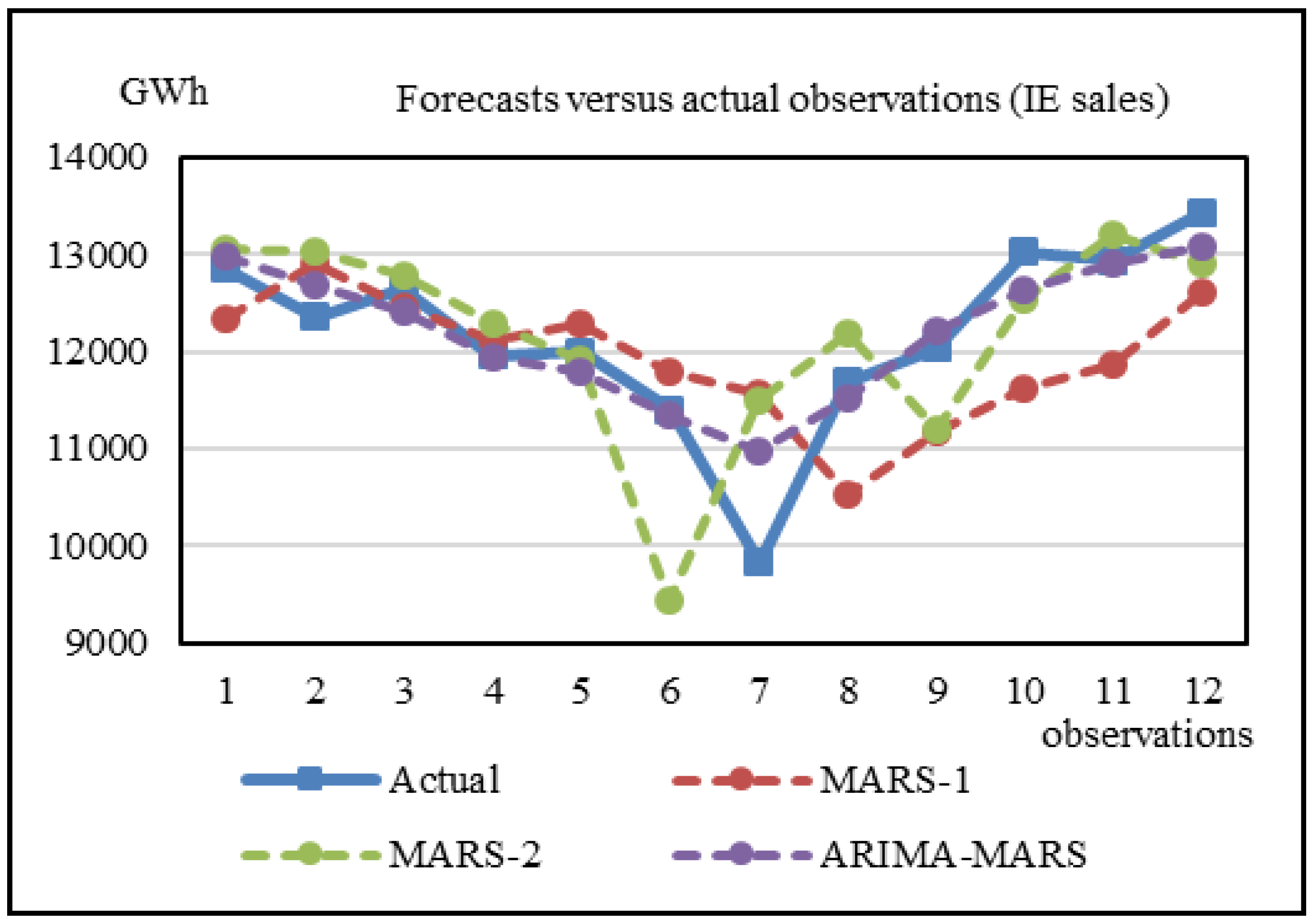
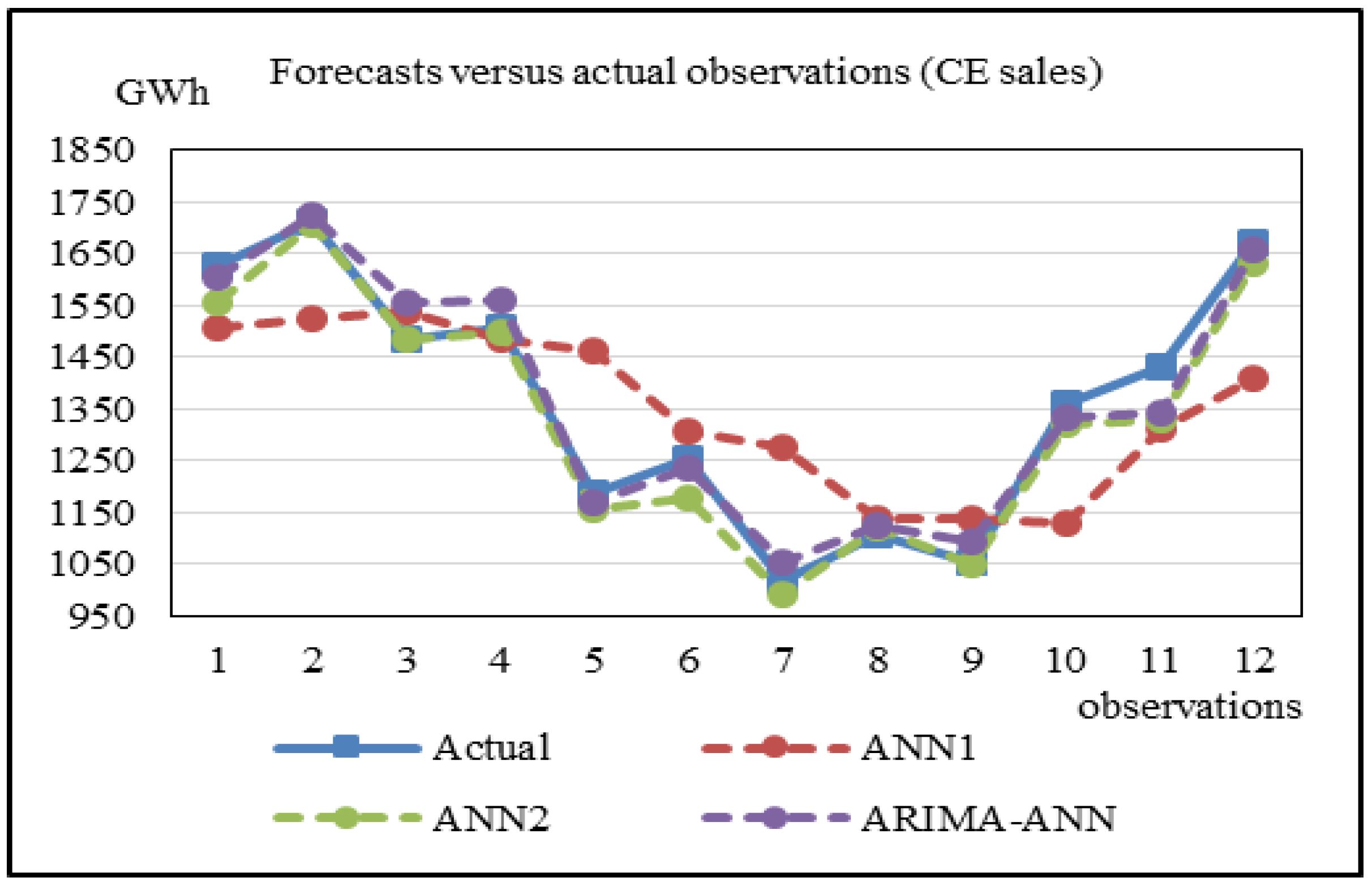
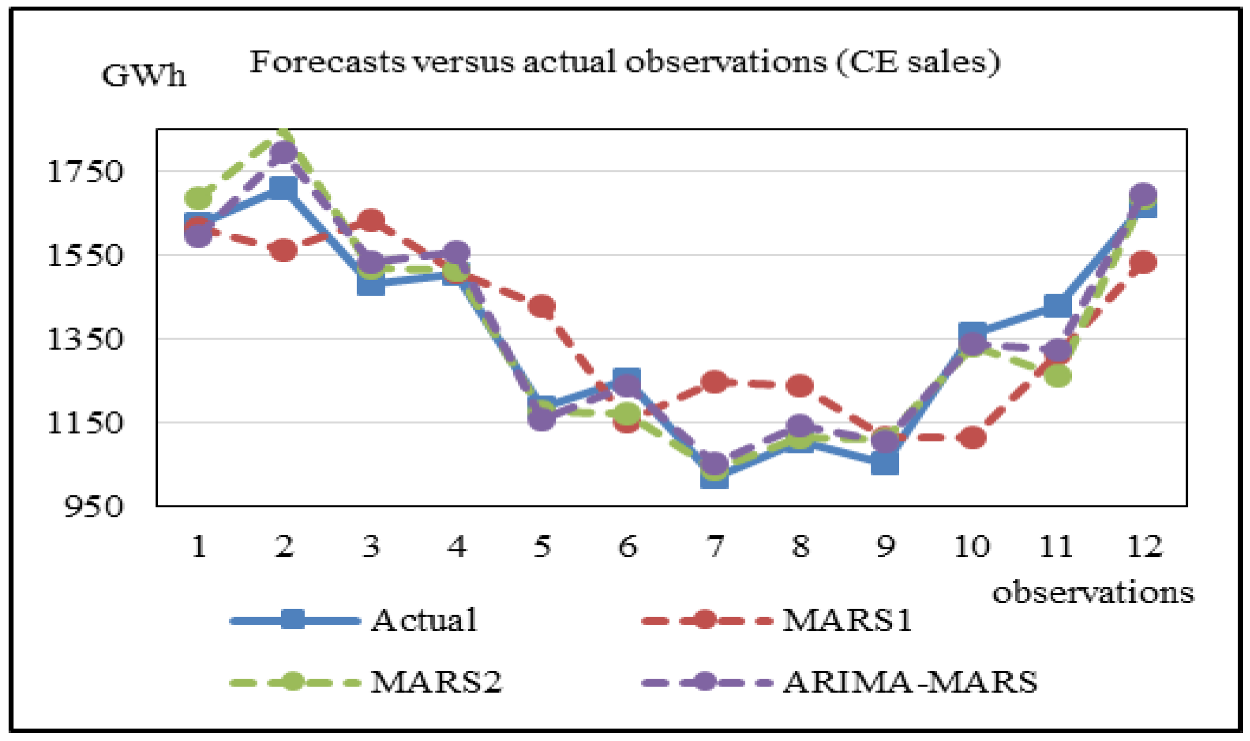
Figure 6 shows the forecasts of IE sales obtained by using MARS-1, MARS-2, and the proposed ARIMA-MARS models for the last twelve testing records. Again, we can observe that the forecasts of the ARIMA-MARS model are closer to the actual observations. Similar results were found for the cases of RE and CE sales. That is, the forecasts of the proposed hybrid models are closer to the actual observations. These findings can be observed in
Figure 7,
Figure 8,
Figure 9 and
Figure 10.
5. Conclusions
For forecasting, typical soft computing approaches need proper explanatory variables to make predictions. However, proper explanatory variables are sometimes difficult to capture, and it is not feasible to obtain the future values of these variables.
Electricity sales forecasting is a challenging task and has drawn considerable attention over the past decades. Consequently, this study investigated hybrid ARIMA-ANN and ARIMA-MARS models for forecasting three types of electricity sales in Taiwan. ARIMA modeling was used as the FST and the significant self-predictor variables were selected by ARIMA. Instead of using unavailable explanatory variables, the self-predictor variables were considered as the inputs for ANN and MARS modeling. The proposed ARIMA-ANN and ARIMA-MARS models were compared with single ANN-1, ANN-2, MARS-1, and MARS-2 models using MAPE, MAD, and RMSE values as performance criteria. The experimental results show that the proposed hybrid ARIMA-ANN and ARIMA-MARS models are good alternatives for electricity sales forecasting since both have good forecasting performance.
Because it is difficult to fully capture the characteristics of real energy data, hybrid modeling should be an acceptable and practical modeling approach. Most importantly, how can soft computing models perform prediction if the proper explanatory variables are not available? Accordingly, the primary contribution of the proposed hybrid models is their ability to provide predictions of electricity sales without requiring extensive effort to obtain the future values of explanatory variables.
Multistep forecasts were considered in this study. The proposed models could handle several months-ahead or one year-ahead forecasts. The modeling process in this study can serve to guide the development of models for electricity sales forecasting in other countries. Although the dataset was collected from January 2006 to July 2016, we believe that the hybrid models will continue to outperform the single-stage models, no matter when our approach will be put in a real production environment.
In this study, the case of d = 0 in ARIMA cay be interpreted as the lack of a trend, which may be because of the economics of an already industrialized country. It is interesting to know if d = 0 still holds for a developing country with a sharp upward trend; this issue needs further investigation by applying the ARIMA technique to electricity sales data for other countries. Additionally, we used 12 inputs (i.e., from
yt-1 to
yt-12) for the second ANN and MARS designs in this study. Because considerable inputs may lead to overfitting problems, we did not include more past seasonal components in our design. However, it may be a good practice to use a few of the past seasonal components (i.e.,
yt-24,
yt-36, or
yt-48) in future ANN or MARS designs. Also, because soft computing modeling is more powerful in capturing nonlinear relationships between input and output, the future studies may use the White test [
46] or Teräsvirta test [
47] to see whether a linearity is rejected or not before attempting nonlinear modelling. Finally, the combination of ARIMA and other forecasting techniques, such as support vector regression or extreme learning machine, to improve forecasting performance can be further investigated in future studies.


