1. Introduction
In recent years, more and more countries have the lower fertility rates, which lead to ageing populations [
1]. The shortage of labor is anticipated, and this will be a serious social problem soon. Consequently, to lead more convenient and safety lives, as well as to free young labor, robots are highly expected to support the daily life of humans at homes, offices, hospitals, and welfare facilities in the years to come [
2]. Furthermore, with a rapidly increasing number of disabled people who need daily life help, life support robots to take caregivers’ roles are increasingly desirable to assist such people by endowing as much independence as possible [
3]. Hence, many kinds of life support robots are being developed [
4,
5,
6]. In the authors’ laboratory, a goods transport robot with automatic moving function based on a mobile platform has been developed [
7].
To freely move in the narrow indoor environment, the mobile platform has the omnidirectional movement function by using three omnidirectional wheels. The mobile platform is a kind of typical three-wheel mobile robot, which consists of batteries, motors, motor drivers and controller. Note that the holonomic property enables robots to simultaneously self-rotate with the translational motion on a straight line. This capability works to an advantage over other types of robots in transport, tracking, and other missions in the uncertain and changing narrow indoor living environment. Since that the robot is working in a narrow indoor living environment, the precise tracking is vital. Moreover, the robot is powered by the batteries carried by itself; therefore, energy constraints are critical to the service time of the indoor carrier robots. Consequently, a high accuracy tracking control strategy considering energy optimization is necessary.
Several researchers have concentrated on the motion control of omnidirectional mobile robot owing to its highly coupled and random nonlinear dynamics, which is challenging for high-performance control system design [
8,
9,
10]. As a critical performance, path and trajectory tracking has been studied extensively; for example, adaptive polar-space motion control [
11], integral sliding mode control [
12], hierarchical improved fuzzy dynamic sliding-mode control [
13], motion control switching between two robust controllers [
14], kinematic control combined with an integral sliding mode controller [
15], robust adaptive tracking control [
16], and model-predictive control with friction compensation [
17], have been developed to improve tracking performance. Specifically, the authors of [
11,
15,
16] investigated the adaptive, robust, and sliding mode control methods for the trajectory tracking and path following of omnidirectional mobile robot with parameter variations and uncertainties. However, they conducted studies using only the kinematic model. The authors of [
12,
13,
14,
17] developed the controller based on the robot’ dynamic model. However, they used the simplified dynamic model omitting the actuator motor dynamics. Few studies about path and trajectory tracking of omnidirectional robot have been done based on the dynamic model with consideration of the actuator motor dynamics. The indoor carrier robot for human support mainly works in a narrow, complex surrounding environment and needs contact with human beings. Therefore, the robot tracking systems are often affected by disturbances and the uncertainty of parameters in a vibration environment, which is more challenging. Moreover, most studies have not considered the energy optimization problem.
Robot systems are often powered by batteries; therefore, they are easily subjected to energy consumption efficiency problem, which significantly affect the operation time and feasibility in the works. Recently, with the development of robot technology, robot systems with high energy consumption have become important research topics [
18,
19,
20,
21,
22,
23,
24,
25,
26,
27,
28,
29,
30]. An improved holistic approach, which adopts a hybrid heuristic accelerated by using multicore processors and the Gurobi simplex method for piecewise linear convex functions, is proposed to minimize energy consumption for the industrial robotics [
18]. An energy consumption optimization scheme to determine the optimal base position and joint motion of a manipulator is proposed [
19]. A novel multi-objective optimization method is developed for power optimization of a snake robot, which applies a particle swarm optimization combined with the pareto fronts method [
20]. Several researchers focused on the energy optimization of biped walking robots, including the constrained quadratic programming and neuro-dynamic-based solver [
21], a novel systematic architecture and algorithm of gait control for energy-efficiency optimization [
22], and energy-optimal motion planning with kino-dynamic constraints [
23]. Furthermore, energy optimization for mobile robots by path planning has drawn wide concern recently [
24,
25].
Note that few of the above studies consider the mobile robots’ energy optimization problem [
26,
27]. Furthermore, these rare studies on mobile robots’ energy optimization only consider the path planning method [
28,
29,
30]. However, the problem of motion performance oriented to pathing tracking of a given path is neglected, which is crucial, as depicted above. In the case of power efficiency, designing a controller to achieve accurate tracking with fast and smooth response is not trivial. To our knowledge, no results considering both the energy efficiency and tracking accuracy for mobile robots have been reported. Consequently, determining how to maintain reliable tracking and ensure long-term autonomy works in the case of disturbances and the uncertainty of parameters in a vibration environment is a worthwhile endeavor.
Motivated by the above observations, the main contributions of this paper are as follows:
- (1)
Since a dynamic model can more exactly formulate the driver-motion mechanism and the performance of actuator motor has a great influence on the performance of robot motion, in this paper, a new dynamic model considering simultaneously the mechanical and electrical systems for the indoor carrier robot is constructed. This new dynamic model is constructed by considering all parameter uncertainties and disturbances.
- (2)
A path tracking controller combining an acceleration feedback controller with an improved robust compensation to successfully deal with the disturbances and the parameters changes is proposed. Especially, we introduce a time-varying decoupling-inverse matrix into the robust compensation based on the dynamic model, which is especially critical in the effectiveness of the compensation and robustness.
- (3)
The proposed controller is proven to be globally asymptotically stable via the Lyapunov stability theory and the tracking error satisfies a specified robust specification, which is observed in a small neighborhood of zero. Considering the special application of the robot, the simulation results demonstrate the efficiency of the proposed scheme, while the new controller was validated by a path tracking experiment subjected to narrow, complex surrounding indoor environment.
The remainder of this paper is organized as follows.
Section 2 describes the design of the structure and the kinetics analysis of the indoor carrier robot.
Section 3 presents the design of the robust path tracking controller. The stability, tracking and energy consumption performance analysis are presented in
Section 4.
Section 5 and
Section 6 show the simulations and experiment using the proposed method, respectively. Finally, we conclude this paper and state possible future research in
Section 7.
2. Structure of the Indoor Carrier Robot and Its Modeling
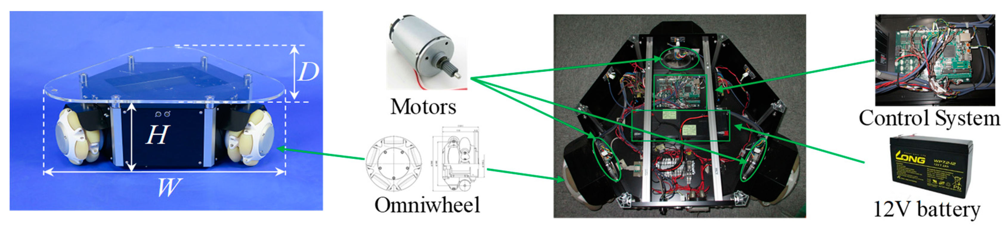
In this section, we introduce the structure of the indoor carrier robot and establish its dynamic models including actuators. An overview of our indoor carrier robot is shown in
Figure 1. Three compact omni wheels are installed at the bottom corners of the robot to provide the robot with omnidirectional movement and thus achieve free movement in a narrow space. The three wheels are independently driven by three highly efficient, permanent, magnet-activated direct-current (DC) motors.
Figure 2 shows two usage examples of this robot. In
Figure 2a, the robot helps the caregiver to carry the bookshelf to the bedridden person, while
Figure 2b shows the robot carrying a package to the bedridden person. From the usage example of this robot, we notice that, when performing its task, the robot needs to go across the narrow places such as a door frame (as shown in
Figure 2b). Therefore, in this condition, we must ensure the robot’s tracking accuracy to avoid colliding with the door frame. Moreover, the energy for indoor carrier robot is stored in the batteries that it carries, and this finite energy is consumed while performing the mission. Thus, to lengthen the use time of indoor carrier robot, strategies for reducing the energy of consumed by motors are desirable.
The values of the physical parameters of the indoor carrier robot are given in
Table 1. The height of this movement platform is 0.275 m. Three omnidirectional wheels enable the support robot to move in any direction with the same orientation and free rotation. The maximum speed of the support robot is 1.96 m/s.
2.1. Modeling in Mechanical Systems
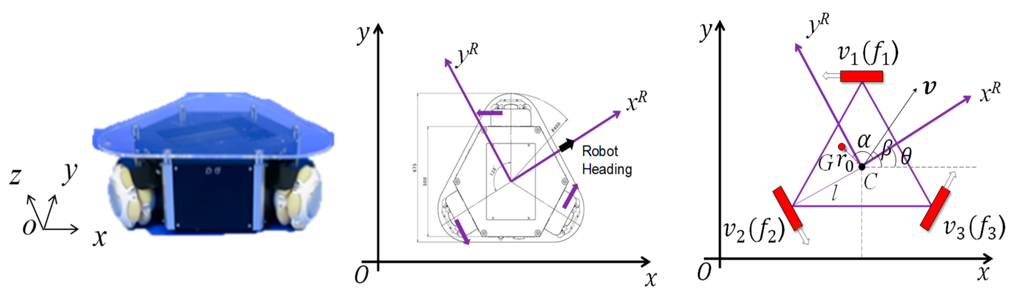
A schematic structure of the robot is shown in
Figure 3. The kinematic and dynamic model analysis of the nonlinear system was carried by using the coordinate system shown in
Figure 3.
In
Figure 3, Σ(
x,
O,
y) is the absolute coordinate system; Σ(
xR,
C,
yR) is the robot coordinate system;
θ is the orientation of the support robot;
C denotes the position of the geometric center;
G is the position of the center of gravity considering the effect of loads;
r0 is the distance between the
G and the
C;
α is the angle between
xR axis and CG, which denote the offset angle of the center of gravity in the robot coordinate system;
v is the speed of the indoor carrier robot;
β is the moving direction of the robot;
vi (
i = 1, 2, 3) is the speed of each omni wheel;
l denotes the distance from the center of the robot to each omni wheel; and
f1,
f2, and
f3 are the driving forces of the three driving wheels.
Using the coordinate system shown in
Figure 3, a kinematic analysis was carried out. The kinematic equation is shown in Equation (1) [
7].
where
where
and
are the
x and
y components of the lift support robot’s velocity at center position, respectively.
According to the coordinate system shown in
Figure 3, we analyzed the movement relationship between
C position and
G position, which is given as follows.
where
Considering the robot is carrying some goods, according to the rigid body dynamics, the motion of robot at center of gravity is given as follows [
7]:
where
where
M is the mass of the indoor carrier robot,
m is the mass of goods,
I is the inertial mass of the robot, and
is the inertia mass caused by
m.
are the
x and
y components of the lift support robot’s acceleration at
G, respectively;
is angular acceleration of the robot around
G; and
ffriction1,
ffriction2, and
ffriction3 are the friction forces on the three wheels. The robot’s primitive load and center of gravity parameters are shown in
Table 2.
According to Equation (2), we can get the robot’s acceleration relation between
C and
G position is
where
is the time differentiation of the relation matrix
.
Rearranging the dynamic in Equation (3) based on Equation (4), we can obtain the robot’s dynamics at position center position as the following [
7].
Remark 1. In practical applications, the difference of the load and the deformation of the mechanical structure, the coupling relationship between each force and robot’s motion (KG(θ)), center of gravity (r0, α) and mass of load (m) shown in Table 2 are changed. In addition, the friction is also nonlinear-time varying. These problems will lead to model perturbation in mechanical systems. The dynamic model in Equation (5) was constructed by considering the deformation of the mechanical structure, center-of-gravity shift, load changes and friction. 2.2. Modeling in Electrical Systems
It is assumed that the three DC motors have the same armature resistance
Ra, back-emf constant
ke, torque constant
kt, and gear ratio
n, as shown in
Figure 4.
To simplify the dynamics, we ignore the inductance of the armature circuits because the electrical response is generally much faster than the mechanical response. The electrical circuit of the DC motor of each wheel is shown in
Figure 4. Letting
Vs be the battery voltage, the armature circuits of both motors are described by [
31]:
where
I = [
i1 i2 i3]
T denotes the armature current vector,
U = [
u1 u2 u3]
T denotes the normalized control input vector, and
ω = [
ω1 ω2 ω3]
T represents the angular velocity of each wheel. Superscripts 1, 2, and 3 correspond to the three motors in
Figure 2, respectively.
In addition, the dynamic relationship between angular velocity and motor current, considering inertia and viscous friction [
32], becomes
where
Fv is the viscous friction coefficient and
J = diag{
J1,
J2,
J3} is the equivalent inertia matrix of the motors, which is symmetric. The values of the physical parameters of the drive motors are given in
Table 3.
Remark 2. In practical applications, the physical parameters of motors, Ra, ke, kt, and J will change with time and environment. This leads to the parameter perturbation problem, which will affect the control accuracy of the robot tracking system. Furthermore, the viscous friction Fv· ω will also affect the tracking accuracy. Therefore, we need to design proper controller to address these problems.
2.3. Robot Dynamics Combining the Mechanical and Electrical System
From Equations (6) and (7), the robot dynamic, considering the electrical circuit, can be written as:
Both sides of Equation (8) are divided by the radius of wheel
r; since
and
, the driving force can be presenting by the control input vector and angular velocity.
Then, putting Equations (1) and (9) into the Equation (5), we can get the robot’s dynamic model considering electrical system as follows:
Remark 3. The dynamic model of the previous study only considered the mechanical system, ignoring the effects of the electrical system. Therefore, in this paper, we take the electrical system into the consideration to improve the control accuracy, as shown in the model in Equation (10).
3. Tracking Control Strategy Design Considering Energy Optimization
The purpose of the present study was designing a feedback robust controller that could track the predefined paths to ensure that the robot can transport goods from an arbitrary initial position to the destination position when the robot is in an environment with uncertainty of center of gravity shift caused by goods and with random parameters. At the same time, the goal was to minimize the energy consumption.
Remark 4. Indoor carrier robot is a class of typical wheeled robots that have omnidirectional movement function. To operate effectively in real-word applications, the control algorithm strategy must guarantee the robot can precisely follow a predesigned path. However, in practical applications, the various uncertainty factors including friction, load force, robot parameters perturbation, load change, center-of-gravity shift etc. seriously affect the tracking accuracy of the robot. Therefore, the design of the robust controller considering theses uncertain is important.
To analyze the robot system and design the control law, we first simplify the dynamics in Equation (10) as:
where
We assume that all these uncertainty factors can be treated as the additive model perturbation, therefore we decompose
M1 and
M2 based on the structure uncertainty characterize into the nominal part
,
and norm bounded perturbation part
,
. Therefore, the dynamic model in Equation (11) can be rewritten as:
Let the desired motion trajectory be
XCd, and the actual motion trajectory be
XC. Therefore, we define the tracking error as follows:
The purpose of the present section is to design a feedback robust controller such that the tracking error e and its time derivative tend toward zero as much as possible, while minimizing the energy consumption and maintaining all other signals in the closed-loop system to be probability bounded.
For the dynamic in Equation (10), a feedback robust controller with the compensation term is proposed.
where
KD = diag(
kDx,
kDy,
kDθ) and
KP = diag(
kPx,
kPy,
kPθ) are the design parameters.
UH is the robust compensation term. Then, putting the control input in Equation (14) into the dynamic in Equation (11), the following equation is obtained.
Let all the parameter perturbation and model perturbation be the norm bounded perturbation
where
γ > 0 denotes the upper bound of the parameter and model perturbation Then, Equation (15) can be rewritten as
Next, we design the robust compensation term
UH to ensure the robot’s
H∞ performance index. First, we let the state vector of the robot tracking system be as follows.
Then, we can get the following state equation.
Equation (19) can be rewritten as
Next, we design the
H∞ compensation control input as
where
R is a given positive definite symmetric matrix and
P is the design control parameter, which is a positive definite symmetric matrix get by solving a Riccati equation as follows.
where
γ > 0 is a given constant to determine the
H∞ stiffness to the parameter uncertainty and external disturbance.
Q is a positive set constant matrix, which satisfies the following inequality:
Figure 5 shows the robust feedback tracking control system.
6. Experiments and Discussion
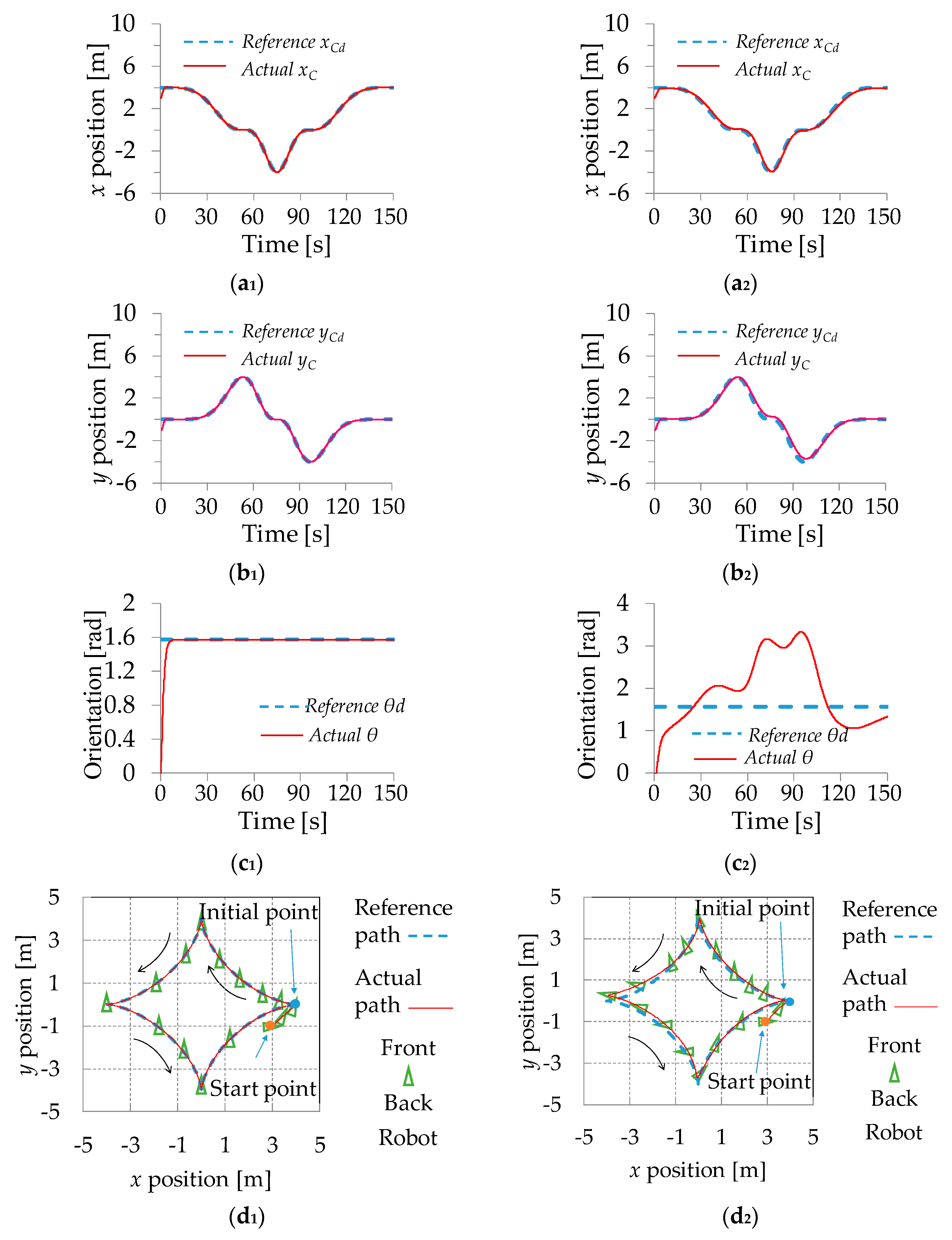
The effectiveness of the proposed method was validated by experiments. The robot was set to track a circle path where the center and the radius were (0 m, 1 m) and 1 m, respectively. The desired trajectory is given as:
The initial position of the robot was (0 m, 0 m, 0 rad). To demonstrate the superiority of the robust controller, path tracking using a controller without robust compensation was also conducted. The two experimental path tracking results are shown in
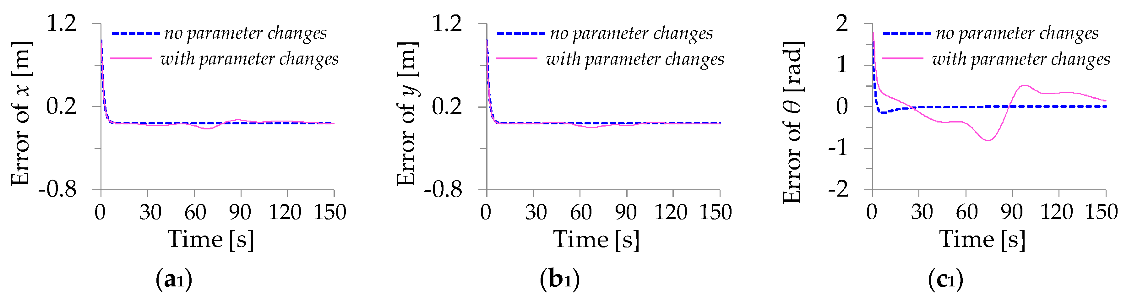
Figure 12, while the trajectory tracking errors of these two controllers are shown in
Figure 13.
Figure 12 shows that satisfactory output tracking control was achieved. In particular, the tracking errors are significantly decreased using the designed robust compensation, as shown in
Figure 13, which clearly indicates that the proposed controller enabled the robot to track the desired path despite parameter uncertainties and maintain good tracking results compared with the controller without the robust compensation. These results suggest that the controller can self-regulate its output values to adapt to changes in robot parameters. The control inputs are shown in
Figure 14. Compared with the control inputs shown in
Figure 14, the control inputs apparently changed to compensate for the varying friction. More specifically, we notice that the control inputs in
Figure 14a are slightly larger than those in
Figure 14b at the beginning. This is the self-regulating behavior adapting to the initial friction and uncertainty, which enables the initial errors of the proposed method to be smaller than those using the non-robust controller, as shown in
Figure 13.
u1 is rather larger around 2 s and 4.3 s, while
u3 is significant around 3 s,
u2 is slightly larger around 0.9 s in
Figure 14a. These are some self-regulating behaviors adapting to the increased friction or robot parameter changes. Further, the control inputs in
Figure 14a are less than those in
Figure 14b during other time intervals, which show the energy-saving performance.
To specifically show the energy conservation of the proposed method, we quantitatively compared the two controllers based on these experiments. The energy consumption during experiments is calculated by . The robot consumed 105.69 kJ energy based on the robust controller while consumed 129.90 kJ energy when using the non-robust one. This result further shows the energy-saving performance of the proposed method.
To further show how well the proposed controller performs in a practice environment, a desired path that complies with a practice application in an actual family environment was designed to be tracked. The robot carried express goods from the vestibule to nearby the bed, as shown in
Figure 15. It can be noticed that the robot needed go through a door frame whose width is 1.0 m, while the width of the robot is 0.733 m, as mentioned above. Hence, the path tracking error must be within 0.133 m, otherwise the robot would collide the door frame.
Four experiments were performed including path tracking experiments using proposed controller with and without goods, and the compared experiments using controller (non-robust compensation one) under the conditions of with and without goods. As with previous experiments, the control parameters of the two controllers were adjusted under the condition of without goods. The path tracking results are shown in
Figure 15.
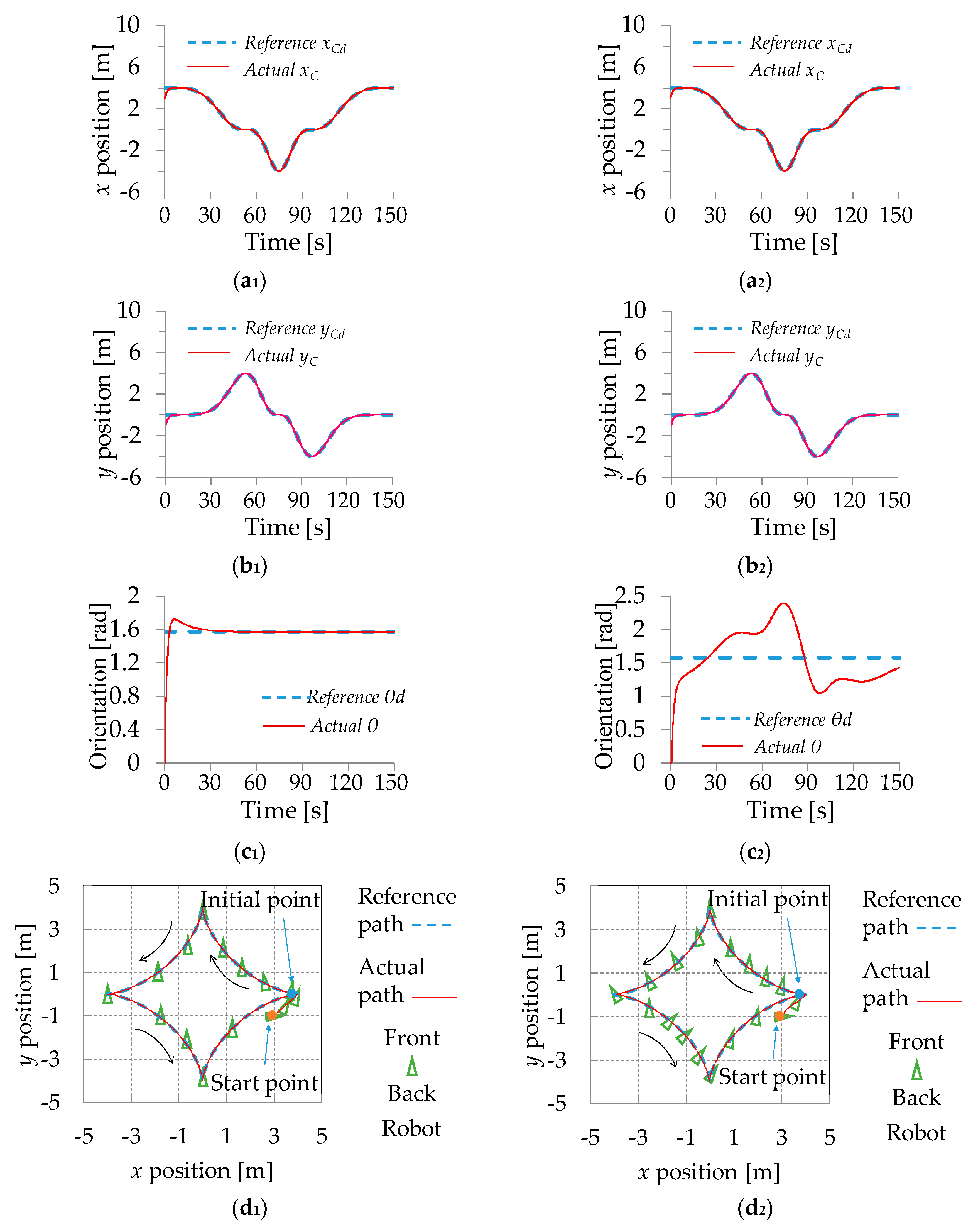
Figure 16a
1 shows that the robot can smoothly track the desired path while the maximum path tracking error in door frame (narrowest space) is 0.03 m. This result indicates that the robot can smoothly go through the door frame based on the proposed controller. Furthermore, the maximum path tracking error is 0.08 m even if the robot has some load (
Figure 16a
2). This result suggests that the proposed controller can guarantee the robot’s smooth movement even with parameter changes in narrow spaces. On the contrary,
Figure 16b
1 shows the maximum path tracking error is 0.0117, which indicates that the robot has an almost permittable tracking performance using the non-robust compensation controller by properly adjusting the control parameters. However, when the robot has some load, the tracking error is 0.33 m (
Figure 16b
1). The robot would collide the door frame in this condition. The experimental results show that the robot can smoothly move in the corridor and go through the door frame based on proposed controller, even with parameter changes.


