Characterization of the Performance of a Turbocharger Centrifugal Compressor by Component Loss Contributions

Abstract

The performance of an automotive turbocharger centrifugal compressor has been studied by developing a comprehensive one-dimensional (1D) code as verified through experimental results and a three-dimensional (3D) model. For 1D analysis, the fluid stream in compressor is modeled using governing gas dynamics equations and the loss mechanisms have been investigated and added to the numerical model. The objective is to develop and offer a 1D model, which considers all loss mechanisms, slip, blockage and also predicts the surge margin and choke conditions. The model captures all features from inlet duct through to volute discharge. Performance characteristics are obtained using preliminary geometry and the blade characteristics. A 3D numerical model was also created and a viscous solver used for investigating the compressor characteristics. The numerical model results show good agreement with experimental data through compressor pressure ratio and efficiency. The effect of the main compressor dimensions on compressor performance has been investigated for wide operating range and the portions of each loss mechanism in the impeller. Higher pressure ratio is achievable by increasing impeller blade height at outlet, impeller blade angle on inlet, diffuser outlet diameter and by decreasing impeller shroud diameter at inlet and blade angle at outlet. These changes may cause unfavorable consequences such as a lower surge margin or shorter operating range, which should be compromised with favorable changes. At lower rotational speeds, impeller skin friction mainly impacts the performance and at higher rotational speeds, impeller diffusion, blade loading and recirculation losses are more important. The results allow the share of each loss mechanism to be quantified for different mass flow rates and rotational speed, shedding new light on which losses are most important for which conditions. For a turbocharger, which must operate over a wide range of conditions, these results bring new insight to engineers seeking to optimize the compressor design as part of an internal combustion engine system.

1. Introduction

Turbochargers play an important role in the automotive industry and despite moves to electrify road transport, turbocharged internal combustion engines still dominate, likely to be the case for some decades particularly for large commercial vehicles [1]. Turbocharger performance, efficiency and stability at different operating conditions are governed mainly by the turbocharger’s compressor and turbine. This study therefore focuses on these components.

Since the compressor affects the operation of the whole engine cycle, it is very important to investigate and improve its performance. In addition, performance investigation is essential after the preliminary design as the validity of the design assumptions should be evaluated before undertaking detailed design and manufacturing.

For an engineer it is very helpful to predict the performance of the machine during the early design stages. Knowledge of the characteristic of compressor, such as efficiency and pressure ratio at different rotational speeds, and also adequacy of surge and choke margin at low and high mass flow rates respectively, results in the ability to adjust the machine design to a more favorable operating domain. After preliminary design in which the overall geometry and dimensions are derived, an accurate and fast performance predictor tool is very useful. 1D analysis is much more suitable and less time consuming than 3D analysis for performance prediction. It has acceptable accuracy and can be readily coded into an in-house program with the graphical user interface (GUI). Above all, its rapid solution makes it ideal as a geometry optimization tool. However after finalizing the design, 3D analysis should be carried out before fabrication and experimental tests since 1D analysis suffers due to the simplifications and generalizations made [2,3].

Several research studies were performed to investigate the loss mechanisms in centrifugal compressors during the period 1950 to 1980 and some mathematical models and correlations are derived and developed. Coppage published relations of losses for ultrasonic flow in centrifugal compressors [4]. Jansen published a method to calculate the flow in the centrifugal impeller by considering entropy generation [5]. Galvas predicted the performance of a centrifugal compressor with channel diffuser in off-design conditions at different mass flow rates [6]. Whitfield and Baines summarized and developed a computational solution to predict the performance of radial flow turbomachines [7]. They derived a general relation for all channels of radial turbomachines by considering gas dynamics and loss experimental relations from the literature. Japikse described the flow in centrifugal compressor components by means of single-zone and jet-and-wake models. He developed a model called the two-zone model considering jet-wake flow pattern at the impeller discharge. In this model the losses are in the wake region and the jet region is considered to have no loss [8]. Oh et al. tested most of previous loss models and compared them with experimental data and two-zone results and presented an optimal set of losses for performance prediction [9].

By developing the computational fluid dynamics (CFD) and increasing the numerical calculation capacity infrastructure, performance prediction of turbomachines using 3D models has been introduced and is widely implemented [10], however the cost of modeling a complete compressor performance map is relatively high and some research has been focused on improvement of the aforementioned models.

Harley et al. focused on a qualitative assessment of many loss models used to predict the compressor map. They concluded that the Galvas loss models, along with the Aungier choking loss would improve the accuracy of prediction but their CFD model for validation does not contain the volute [11]. Fang et al. summarized the empirical models for efficiency and mass flow rates of centrifugal compressors to see the differences for different compressor applications in refrigeration systems and turbochargers [12]. Cicciotti et al. claimed that for developing a model for online applications such as condition monitoring, mean-line algebraic models are the best candidates. They developed a methodology for modifying mean-line models for multistage centrifugal compressors by appropriate selection and adaptation of existing loss correlations in the literature [13]. Wenhai et al. predicted the centrifugal compressor performance using the quasi-one-dimensional formulation coupled with empirical loss models [14].

Taburri et al. presented a mean-line simulation to predict turbocharger centrifugal compressor performance. They considered the inlet, impeller and vaneless diffuser in the model. However they just applied the effect of slip, incidence, friction and heat loss in the impeller section with the results showing the accuracy of their model given in [15]. Zhuge et al. developed a turbocharger simulation method, which models the compressor and turbine using two-zone and mean-line methods respectively. They also determined the key modeling parameters [16].

Besides 1D models, some researchers developed the algorithms to allow machine performance to be predicted from some operational point conditions. Casey and Robinson introduced an engineering method to predict the performance of a compressor at off design conditions based on some limited data at the design point [17]. Chu et al. used a statistical analysis technique to do the same [18].

Using CFD some researchers focused on modifying the loss model coefficients to improve 1D models [19] or modifying the performance of the component through the complete map of the compressor [20,21,22,23,24].

In this research, a set of empirical loss models is selected from the open literature, a comprehensive mean-line analysis procedure considering losses, surge and choke, slip and blockage is generated for inlet duct to volute discharge and a numerical program is developed based on it. Compressor performance characteristics are derived and verified through experimental results for a turbocharger compressor. 3D numerical modeling is also performed to evaluate the accuracy of the developed 1D model. Furthermore the effect of changes in some geometry parameters on performance is observed accordingly. These results show the variation and sensitivity of performance characteristics when design parameters are changed slightly. Mechanisms that are detected as energy loss sources are compared with each other on the operating range of compressor and for different rotational speeds. The results state which loss sources are the most important ones and so allow these to be targeted for reduction. The methodology and results proposed in this paper helps designers to evaluate the designed compressor and choose the strategy of the optimization.

2. 1D Procedure

In order to predict centrifugal compressor performance using mean-line analysis, it is necessary to analyze its components, including inlet duct, impeller, diffuser and volute. To do so, requires marching through the compressor in the flow direction; the ideal stream being modeled by thermodynamic and fluid mechanic relations, then, by implementing loss mechanism relations and correlations, the model becomes more realistic. To do so, a set of empirical models was selected. In this study, models that were physically based were preferred rather than models that were based solely on mathematical correlations. Under the specified geometry, inlet conditions, rotational speed and mass flow rate, stream properties could be calculated at discharge of each component and set for the next component inlet. From the model, velocities, static and total temperature, static and total pressure, efficiency and pressure loss of each component could be calculated.

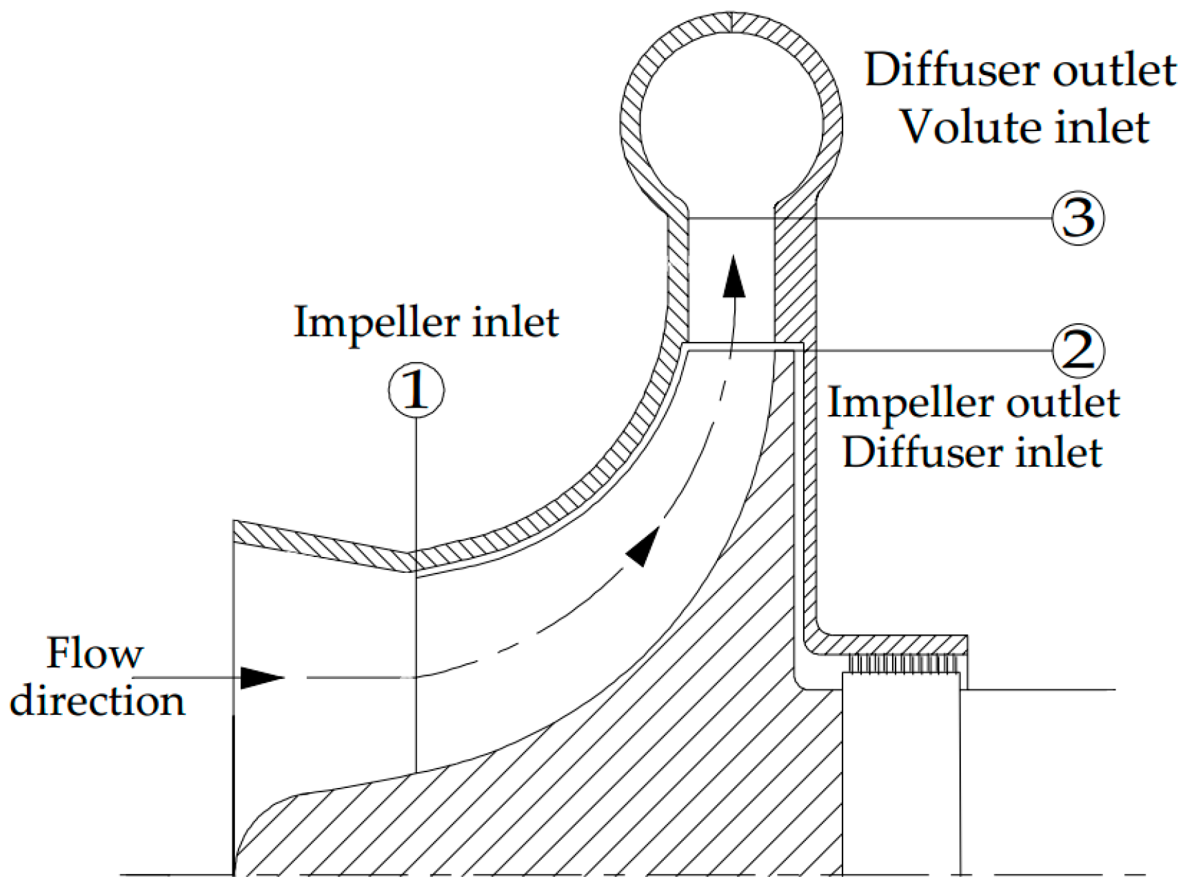
Using mass and energy conservation laws and entropy generation, Equations (1) and (2) can be obtained [7] with 1 and 2 being used for inlet and outlet of each component respectively (see Figure 1). Outlet flow properties can then be calculated with known inlet flow properties.

$$\frac{\dot{m}\sqrt{R{T^{\prime }}_{01}/\gamma }}{A_1{P^{\prime }}_{01}}=\frac{A_2}{A_1}{M^{\prime }}_2\cos {\beta }_2{\left(1+\frac{\gamma -1}{2}{M^{\prime }}_2^2\right)}^{\raisebox{1ex}{$-\left(\gamma +1\right)$}\!\left/ \!\raisebox{-1ex}{$2\left(\gamma -1\right)$}\right.}\cdot \sigma {\left(1+\frac{\gamma -1}{2\gamma R{T^{\prime }}_{01}}\left(U_2^2-U_1^2\right)\right)}^{\raisebox{1ex}{$\gamma +1$}\!\left/ \!\raisebox{-1ex}{$2\left(\gamma -1\right)$}\right.}.$$

(1)

The following sections describe the assumptions and relations considered for the 1D model based on the Equation (1).

2.1. Inlet Duct

At the inlet section, for known ambient conditions, the velocity at the entrance of the impeller was calculated via Equation (2) by simplification of Equation (1) as follows.

$$\frac{\dot{m}\sqrt{R{T}_{01}/\gamma }}{A_1{P}_{01}}=M_1{\left(1+\frac{\gamma -1}{2}{M}_1^2\right)}^{-\left(\gamma +1\right)/2\left(\gamma -1\right)},$$

(2)

in which, T₀₁, is equal to the ambient total temperature as no work is exerted to flow in the duct and P₀₁ is unknown, thus, it is set equal to the ambient total pressure in the first step, then, total pressure loss in the duct was calculated from the Darcy–Weisbach relation [25], the equation was solved when the pressure and velocity become converged.

2.2. Impeller

For predicting the impeller outlet conditions, the unknown parameter in RHS (Right Hand Side) of Equation (1) includes the outlet velocity direction, β₂, the energy loss factor, σ, and the relative Mach number, M₂′. The outlet velocity angle is obtained from Equation (3) [7]:

$$\sin {\beta }_2=\frac{\frac{-U_2\left(1-\mu \right)}{W_2}+\tan {\beta }_{B2}{\left[1+{\tan }^2{\beta }_{B2}-\frac{U_2^2{\left(1-\mu \right)}^2}{W_2^2}\right]}^{1/2}}{1+{\tan }^2{\beta }_{B2}},$$

(3)

in which the slip factor is [26]:

$$\mu =1-\frac{\sqrt{\cos {\beta }_{B2}}}{Z_B^{0.7}}.$$

(4)

The energy loss factor, σ, is associated with all mechanisms in the impeller, which results in entropy generation, Δs. This factor is defined as Equation (5) for the impeller with respect to the impeller enthalpy loss coefficient, Δq_1–2 [7].

$$\sigma =\exp \left(-\Delta s/R\right)={\left(1-\frac{\gamma -1}{\gamma R{T^{\prime }}_{02}}{U}_T^2\Delta q_{1-2}\right)}^{\gamma /\left(\gamma -1\right)}.$$

(5)

Impeller losses can be divided into incidence loss at entrance (Δ_qi), skin friction loss (Δq_sf), diffusion and blade loading loss (Δq_bl), mixing loss (Δq_mix), clearance loss (Δq_cl), choke loss (Δq_ch), disk friction loss (Δq_df) and recirculation loss (Δq_rc). Hence the impeller loss is the summation of these losses.

$$\Delta q_{1-2}=\Delta q_i+\Delta q_{sf}+\Delta q_{bl}+\Delta q_{mix}+\Delta q_{cl}+\Delta q_{ch}+\Delta q_{df}+\Delta q_{rc}=\frac{h_{02}-h_{02s}}{U_T^2}.$$

(6)

Entrance incidence loss: This is due to difference between the relative flow angle and blade angles at the impeller entrance. Galvas assumes that the whole kinetic energy associated with the change in the tangential component of relative velocity converts to internal energy [6] and presents:

$$\Delta q_i=\frac{{\left(W_1\sin \left(\left|{\beta }_1-{\beta }_{B1}\right|\right)\right)}^2}{2U_T^2}.$$

(7)

Skin friction loss: This is due to shear stresses from impeller channel surfaces. Friction losses in impellers have a similar mechanism to total pressure drop in straight pipes based on a channel with hydraulic diameter and length of d_H and L_H respectively, so skin friction loss is calculated by [5]:

$$\Delta q_{sf}=2C_f\frac{L_H}{d_H}\frac{{\overline{W}}^2}{U_T^2},$$

(8)

where $\overline{W}$, d_H and L_H are [5]:

$$\overline{W}=\frac{2W_2+W_{h1}+W_{s1}}{4},$$

(9)

$$\frac{d_H}{d_2}=\frac{\cos {\beta }_2}{\left[\frac{Z}{\pi }+\frac{d_2\cos {\beta }_2}{b_2}\right]}+\frac{\frac{1}{2}\left(\frac{d_{s1}}{d_2}+\frac{d_{h1}}{d_2}\right)\left(\frac{\cos {\beta }_{s1}+\cos {\beta }_{h1}}{2}\right)}{\frac{Z_B}{\pi }+\left(\frac{d_{s1}+d_{h1}}{d_{s1}-d_{h1}}\right)\left(\frac{\cos {\beta }_{s1}+\cos {\beta }_{h1}}{2}\right)},$$

(10)

$$L_H=\frac{\pi }{8}\left[d_2-\frac{d_{s1}-d_{h1}}{2}-b_2+2L_A\right]\cdot \left(\frac{2}{\frac{\cos {\beta }_{s1}+\cos {\beta }_{h1}}{2}+\cos {\beta }_2}\right).$$

(11)

The friction coefficient, C_f is calculated by following the relation based on the Reynolds number, Re [27],

$$\begin{array}{c}{C}_f=\{\begin{array}{cc}0.0622{\mathrm{Re}}^{-0.2}\hfill & (\mathrm{Re}\ge 3\times {10}^5)\hfill \\ 2.67{\mathrm{Re}}^{-0.5}\hfill & (\mathrm{Re}\le 2\times {10}^5)\hfill \end{array},\\ \mathrm{Re}=\frac{\rho \cdot \overline{W}\cdot D_H}{\mu }.\end{array}$$

(12)

Diffusion and blade loading loss: This loss is due to boundary layer growth, which leads to flow separation and secondary flows. Coppage and Jansen suggested following the relation for estimating this loss [4,5],

$$\Delta q_{bl}=0.05D^2,$$

(13)

in which the diffusion factor, D, is as below [28].

$$D=1-\frac{W_2}{W_{s1}}+0.6\Delta q_{imp}\frac{W_2}{W_{s1}}{\left[\frac{Z_B}{\pi }\left(1-\frac{r_{s1}}{r_2}\right)+\frac{2r_{s1}}{r_2}\right]}^{-1},$$

(14)

$$\Delta q_{imp}=\left(C_{\theta 2}{U}_2-C_{\theta 1}{U}_1\right)/U_2^2.$$

(15)

Mixing loss: As the impeller discharge wake stream mixes with the main stream in the vaneless diffuser space, the energy loss occurs. Johnston presents the following equation [29] for quantifying this loss:

$$\Delta q_{mix}=\frac{1}{1+{\tan }^2{\alpha }_2}{\left[\frac{1-{\epsilon }_{wake}-b^{*}}{1-{\epsilon }_{wake}}\right]}^2\frac{C_2^2}{2U_T^2},$$

(16)

in which, b* is the ratio of diffuser inlet height to impeller outlet height and ε_wake is the wake fraction of blade-to-blade space.

Clearance loss: Fluid leakage from the pressure side to the suction side of the blade results in clearance loss. Jansen presents the following equation for this [5];

$$\Delta q_{cl}=0.6\frac{\epsilon }{b_2}\frac{C_{\theta 2}}{U_T}\cdot {\left[\frac{4\pi }{b_2{Z}_B}\left(\frac{r_{s1}^2-r_{h1}^2}{\left(r_2-r_{s1}\right)\left(1+{\rho }_2/{\rho }_1\right)}\right)\frac{C_{\theta 2}}{U_T}\frac{C_{m2}}{U_T}\right]}^{1/2}.$$

(17)

Disk friction loss: This loss is due to the shear stresses exerted to the fluid trapped in the gap between the rear face of the impeller and the adjacent stationary faces [7];

$$\Delta q_{df}=0.25\overline{\rho }{U}_T{r}_T^2{K}_f/\dot{m},$$

(18)

where K_f is the empirical torque coefficient and defined as below [30]:

$$\begin{array}{c}{K}_f=\{\begin{array}{cc}3.7{\left(\epsilon /r_T\right)}^{0.1}{\mathrm{Re}}^{-0.5}\hfill & (\mathrm{Re}<3\times {10}^5)\hfill \\ 0.102{\left(\epsilon /r_T\right)}^{0.1}{\mathrm{Re}}^{-0.2}& (\mathrm{Re}\ge 3\times {10}^5)\hfill \end{array},\\ \mathrm{Re}=U_T{r}_T/\nu .\end{array}$$

(19)

Recirculation loss: This is due to that part of the fluid with low momentum, which turns back to the impeller after leaving it and receives work another time. Coppage presents the following Equation [4].

$$\Delta q_{rc}=0.02D^2\tan {\alpha }_2,$$

(20)

where D is the diffusion factor and calculated from Equation (13).

Stall and choke: Stable operation is limited by stall at low mass flow rate and choke condition at high mass flow rate. According to Aungier [31], impeller stall occurs when the equivalent diffusion factor, as expressed in Equation (21), exceeds the value of 2.

$$D_{eq}=\frac{1}{2W_2}\left[W_1+W_2+\frac{4\pi r_T{U}_T\left(\Delta q_{imp}+\Delta q_{df}+\Delta q_{rc}\right)}{\left(Z_B+{Z_S{L}_S/L}_B\right)L_C}\right].$$

(21)

At high mass flow rates, the relative Mach number at the impeller throat reaches to 1. In this condition impeller is choked and the pressure ratio falls rapidly. Choke energy loss is calculated from following equation based on Aungier [31].

$$\begin{array}{cc}\Delta q_{ch}=0\hfill & X\le 0,\hfill \\ \Delta q_{ch}=\frac{W_1^2\left(0.05X+X^7\right)}{4U_T^2}\hfill & X>0,\hfill \end{array}$$

(22)

in which X is defined as following [32];

$$X=\frac{\dot{m}}{{\dot{m}}_{ch}}-{\left(11-10\frac{\dot{m}}{{\dot{m}}_{ch}}\right)}^4,$$

(23)

where ${\dot{m}}_{ch}$ is the mass flow, which causes the relative Mach number to equal unity at throat.

Blockage factor: A portion of geometrical impeller exit area is blocked by boundary layer growth. Aungier represented the following equation to calculate impeller blockage, which means the ratio of blocked area to the geometrical area, so the geometrical area is multiplied by (1 − B₂) to calculate flow area [31].

$$B_2=\frac{2U_T^2\Delta q_{sf}}{W_1^2}\frac{P_{01}-P_1}{P_{02}-P_2}\sqrt{\frac{W_1{d}_H}{W_2{b}_2}}+\left(0.3+\frac{b_2^2}{L_C^2}\right){\left(\frac{A_2\cos {\beta }_2}{A_1\cos {\beta }_{th}}\right)}^2\frac{{\rho }_2{b}_2}{{\rho }_1{L}_C}.$$

(24)

2.3. Vaneless Diffuser

Flow in the vaneless diffuser is an unguided swirling flow and since the flow path is long, frictional loss is considerable. Circumferential velocity at diffuser outlet is calculated through the following Equation [33]:

$$\frac{C_{\theta 2}}{C_{\theta 3}}=\frac{r_3}{r_2}+\frac{2\pi C_f{\rho }_2{C}_{\theta 2}\left(r_3^2-r_2{r}_3\right)}{\dot{m}},$$

(25)

in which, C_f, is diffuser friction coefficient and calculated by following [34]:

$$C_f=0.01{\left(1.8\times {10}^5/\mathrm{Re}\right)}^{0.2}.$$

(26)

Having C_θ3 and using velocity triangle at outlet, flow angle can be calculated [7]:

$$\sin {\alpha }_3=\frac{C_{\theta 3}{\left[1+\left[\left(\gamma -1\right)/2\right]M_3^2\right]}^{1/2}}{M_3\sqrt{\gamma R{T}_{03}}}.$$

(27)

On the other hand, the outlet Mach number is calculated through Equation (28):

$$\frac{\dot{m}\sqrt{R{T}_{02}/\gamma }}{A_3{P}_{02}}=\sigma M_3\cos {\alpha }_3{\left(1+\frac{\gamma -1}{2}{M}_3^2\right)}^{-\left(\gamma +1\right)/2\left(\gamma -1\right)}.$$

(28)

Two Equations (27) and (28) with two unknowns α₋₃ and M₃ can be solved to find other flow properties.

Only skin friction is considered for vaneless diffuser energy loss. Coppage represents the following equation to calculate this loss [4]:

$$\Delta q_{2-3}=\frac{C_f{r}_2\left[1-{\left(r_2/r_3\right)}^{1.5}\right]{\left(C_2/U_T\right)}^2}{1.5b_2\cos {\alpha }_2},$$

(29)

and the entropy gain in Equation (29) is determined as follow [7]:

$$\sigma =\exp \left(-\Delta s/R\right)={\left(1-\frac{\gamma -1}{\gamma R{T}_{03}}{U}_T^2\Delta q_{2-3}\right)}^{\gamma /\left(\gamma -1\right)}.$$

(30)

2.4. Discharge Volute

The velocity of volute outlet flow is obtained from mass conservation and based on a constant density assumption from inlet to outlet. Volute losses are considered as losses of kinetic energy associated with circumferential and meridional components of velocity [35].

It is assumed that the kinetic energy associated with meridional velocity of the volute inlet flow is totally lost [35].

$$\Delta h_{3-4,m}=\frac{C_{m3}^2}{2}.$$

(31)

The loss associated with the circumferential velocity was modeled with a sudden expansion and depends on the volute sizing parameter, $\mathrm{SP}=C_{\theta 3}{r}_3/C_4{r}_4$ [35].

$$\Delta h_{3-4,\theta }=\{\begin{array}{ll}\frac{1}{4}\left(C_{\theta 3}^2-C_4^2\right)& (\mathrm{SP}\ge 1)\\ \frac{1}{2}{\left(C_{\theta 3}-C_4\right)}^2& (\mathrm{SP}<1)\end{array}.$$

(32)

So the entropy gain is determined as the following [7]:

$$\sigma =P_{04}/P_{03}=\exp \left(-\Delta s/R\right)={\left(1-\frac{\gamma -1}{\gamma R{T}_{04}}\left(\Delta h_{3-4,m}+\Delta h_{3-4,\theta }\right)\right)}^{\gamma /\left(\gamma -1\right)}.$$

(33)

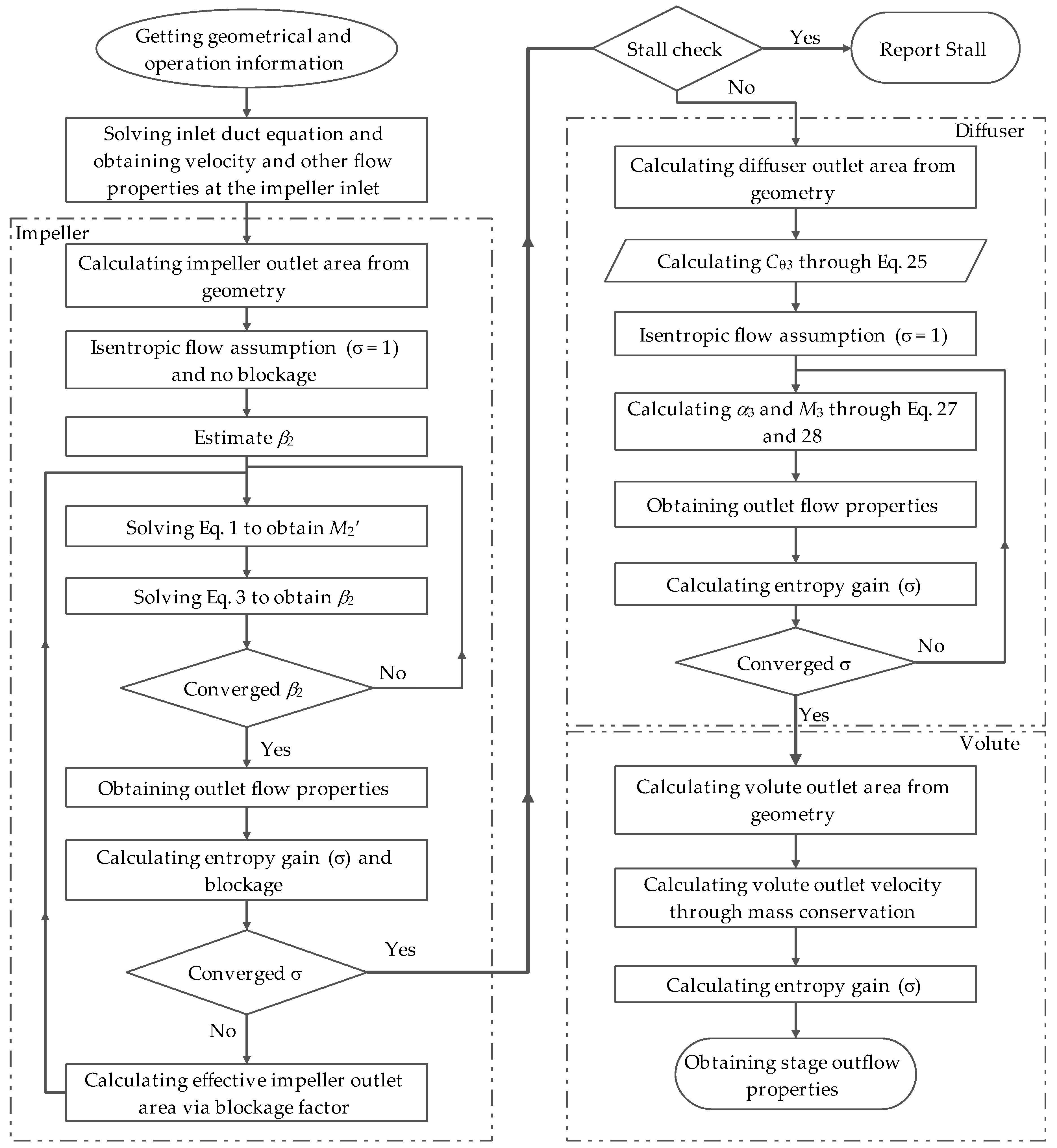
The computational procedure based on the above relations is illustrated in Figure 2. As seen, it is divided to three main blocks i.e., impeller, diffuser and volute and in each block firstly, stream is calculated with no loss (σ = 1) and then losses are calculated through an iterative loop.

3. Compressor Geometry

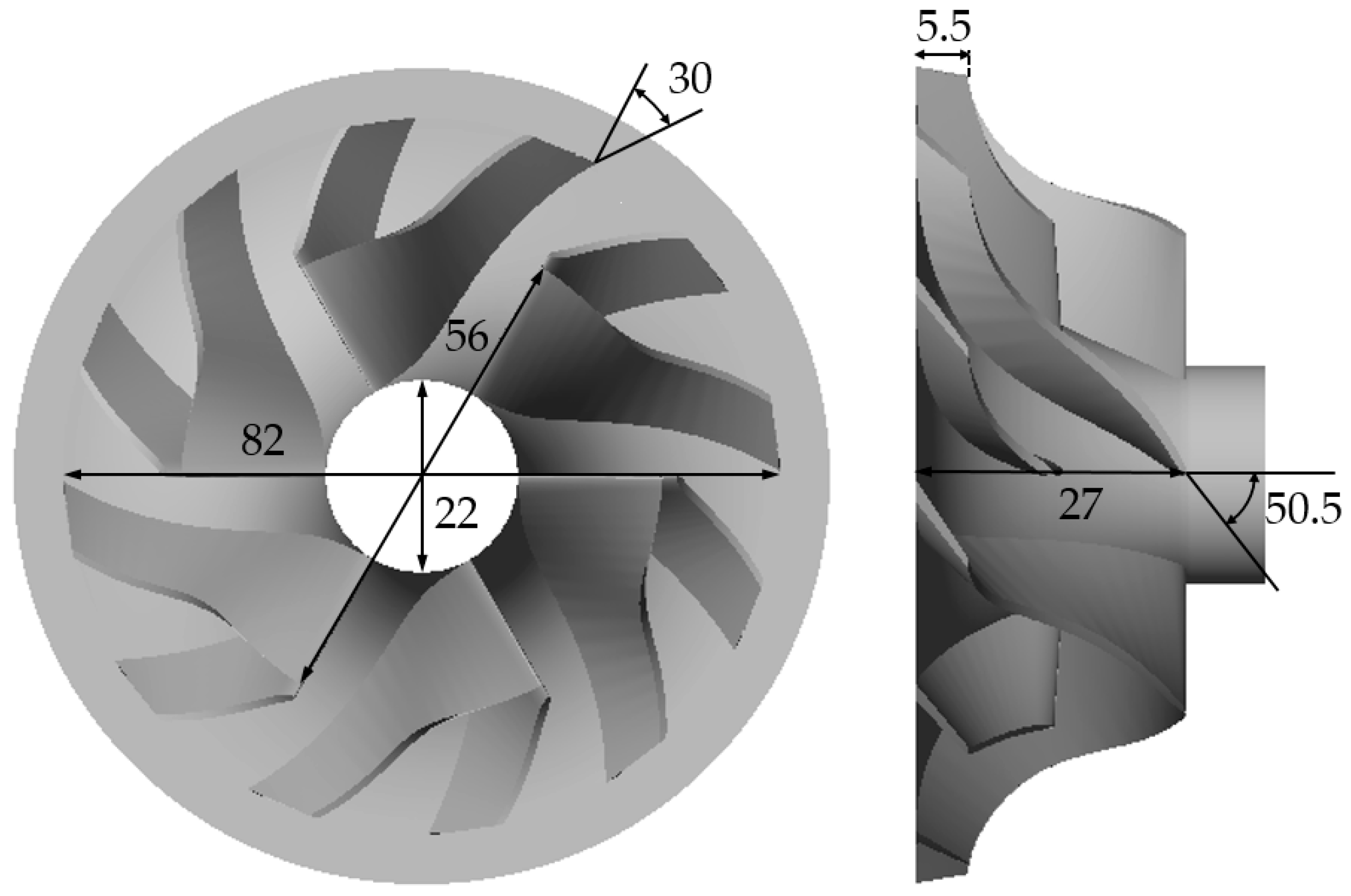
To validate the numerical results, the available experimental test from a results [36,37] for a turbocharger compressor was used. The compressor impeller had six full blades and six splitters. A vane-less diffuser and an overhang volute were the other main components. The main geometrical specifications of the compressor components are tabulated in

Table 1. Geometric specifications of the compressor.

Parameter	Value	Parameter	Value
d1h	22 mm	ZB (ZS)	6 (6)
d1s	56 mm	LA	27 mm
tB1	1.25 mm	ε	0.4 mm
βB1	50.5°	d3	155.5 mm
d2	82 mm	b3	4.27 mm
b2	5.5 mm	d4	194 mm
tB2	1.8 mm	A4	2361 mm2
βB2	−30°

and the geometry is visible in Figure 3.

4. 3D Modeling

3D modeling of the whole compressor components, including inlet duct, impeller, diffuser and volute was also performed for comparison with the results from the 1D developed model. The component geometries were extracted and the CAD file was created for meshing [10,38].

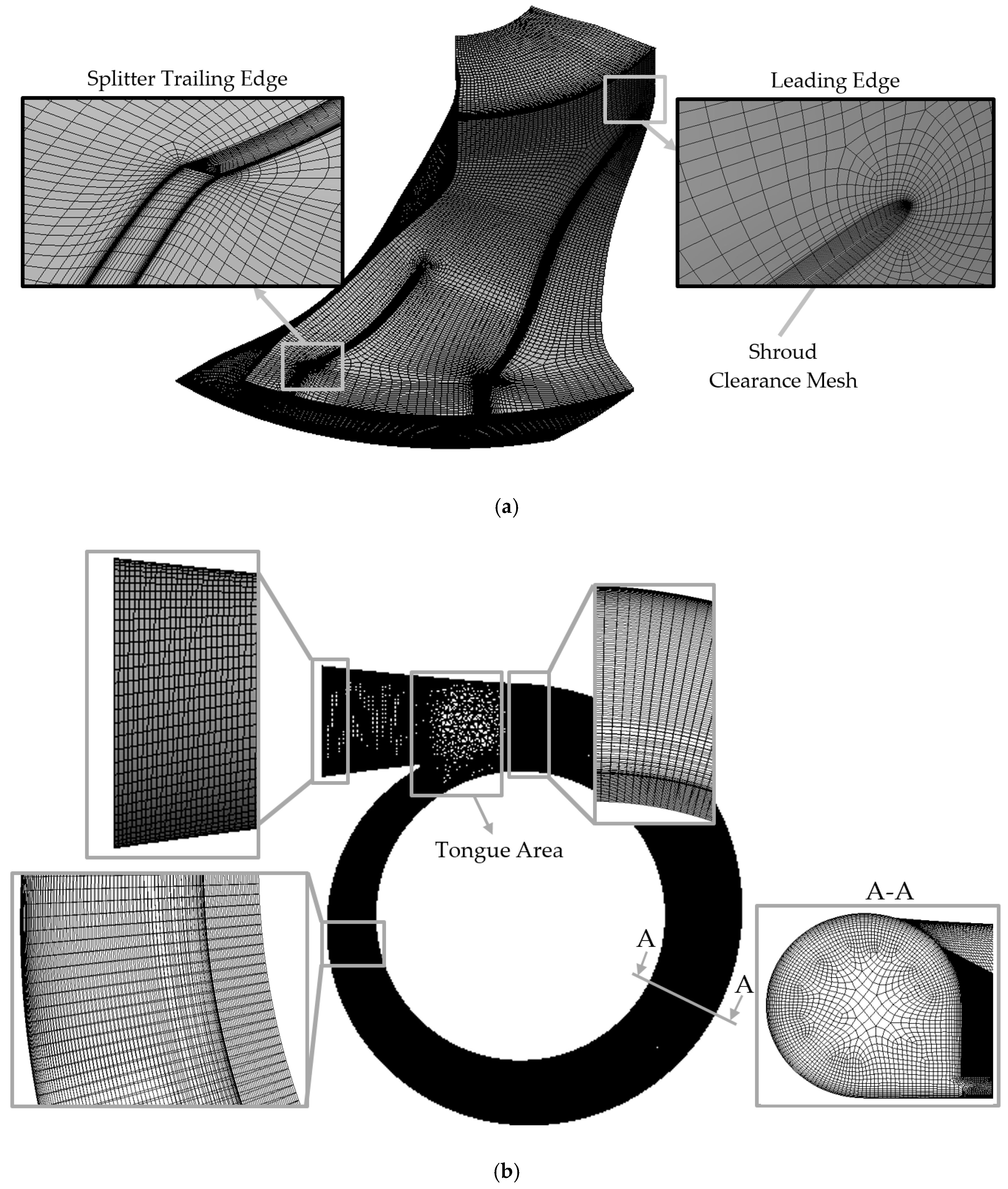
For the inlet section, impeller passage and vaneless diffuser, one passage was considered for modeling and periodic boundaries were used. As visible in Figure 4a, these sections were meshed using structured hexahedral grids. Each passage of impeller included one full blade and a splitter in which the O-type grid was used for leading edge and H-type for the trailing edge of airfoils [39]. Structured mesh aspect ratio quality average was 0.8 and the minimum angle for the 98% of cells was higher than 45 degrees. The expansion factor was limited to 15 and the boundary layer growth rate was set to be 1.15.

For the volute section, three zones were considered for mesh generation as shown in Figure 4b. Mapped hexahedral grids were implemented for the spiral section and the exit cone, however as the tongue zone was the intersection of these two geometries, unstructured tetrahedral elements had to be used in this area with prismatic elements for boundary layers. Minimum edge size for volute mesh was around 0.1 mm and the expansion factor limit and the minimum angle for 98% of cells were 15 and 40 respectively

All components had the boundary layer meshes with seven to 12 layers and the layer growth rate was set below 1.15. First element thicknesses were adjusted to capture flow field with sufficient accuracy with an appropriate y+ in the range of 10 to 30. Wall functions were used to satisfy the physics in the near wall region.

Mesh independency analysis results are shown in

Table 2. Mesh independency analysis.

Mesh No.	No. of Elements	Pressure Ratio		Efficiency
		Value	Error with M4 (%)	Value (%)	Error with M4 (%)
M1	915,000	1.4808	0.64	76.55	5.01
M2	1,600,000	1.4741	0.19	74.44	2.12
M3	2,750,000	1.4714	0	73.07	0.24
M4	4,500,000	1.4714	-	72.89	-

, performed based on the compressor pressure ratio and isentropic efficiency values at 60k rpm rotational speed and 0.09 kg/s mass flow rate. Increasing mesh resolution shows the minimum elements required for giving near constant performance values. Around 750,000 elements per passage were used from the inlet section to vaneless diffuser discharge and near two million elements were used for the volute.

A 3D flow simulation solver was used in which the Reynolds averaged Navier–Stokes equations were solved iteratively with using shear stress transform scheme for turbulence modeling [20,37]. Pressure–velocity coupling was performed by the SIMPLEC method. Atmospheric stagnation conditions were set at the inlet section and the mass flow rate was set at the volute outlet. The Frozen Rotor method was utilized between the rotating and stationary parts to transmit calculated values between zones without variation of the relative positions. The steady state assumption was used for modeling and for minimizing the convergence speed, a time step, which is inversely proportional to the rotation speed was set for each rotational speed of the impeller.

Turbulence intensity was set to 5% at the inlet. Convergence criteria were considered such that the efficiency and pressure ratio reached to a nearly constant value with the maximum residuals for conservation equations reduced to 5.0 × 10⁻⁵.

5. Results and Discussion

In this section, the results are presented. Firstly, numerical models results were compared with each other and verified against experimental data through compressor pressure ratio and efficiency. Secondly, the effect of five main design parameters on the pressure ratio was observed and analyzed and thirdly, loss sources in the compressor were compared and the effect of them on performance was depicted.

5.1. Performance

After fulfilling 1D and 3D numerical models, the results were compared with experimental data. To facilitate this comparison the performance characteristics were used, which were the total to total pressure ratio and the isentropic efficiency defined by following equations.

$$PR=\frac{P_{04}}{P_a},$$

(34)

$$\eta =\frac{T_a\left(P{R}^{\frac{\gamma -1}{\gamma }}-1\right)}{T_{04}-T_a}.$$

(35)

Pressure ratio and isentropic efficiency versus mass flow rate were plotted for different rotational speeds considering surge and choke limits. For the 3D model, the mass flow average at each section was used for calculating the flow properties.

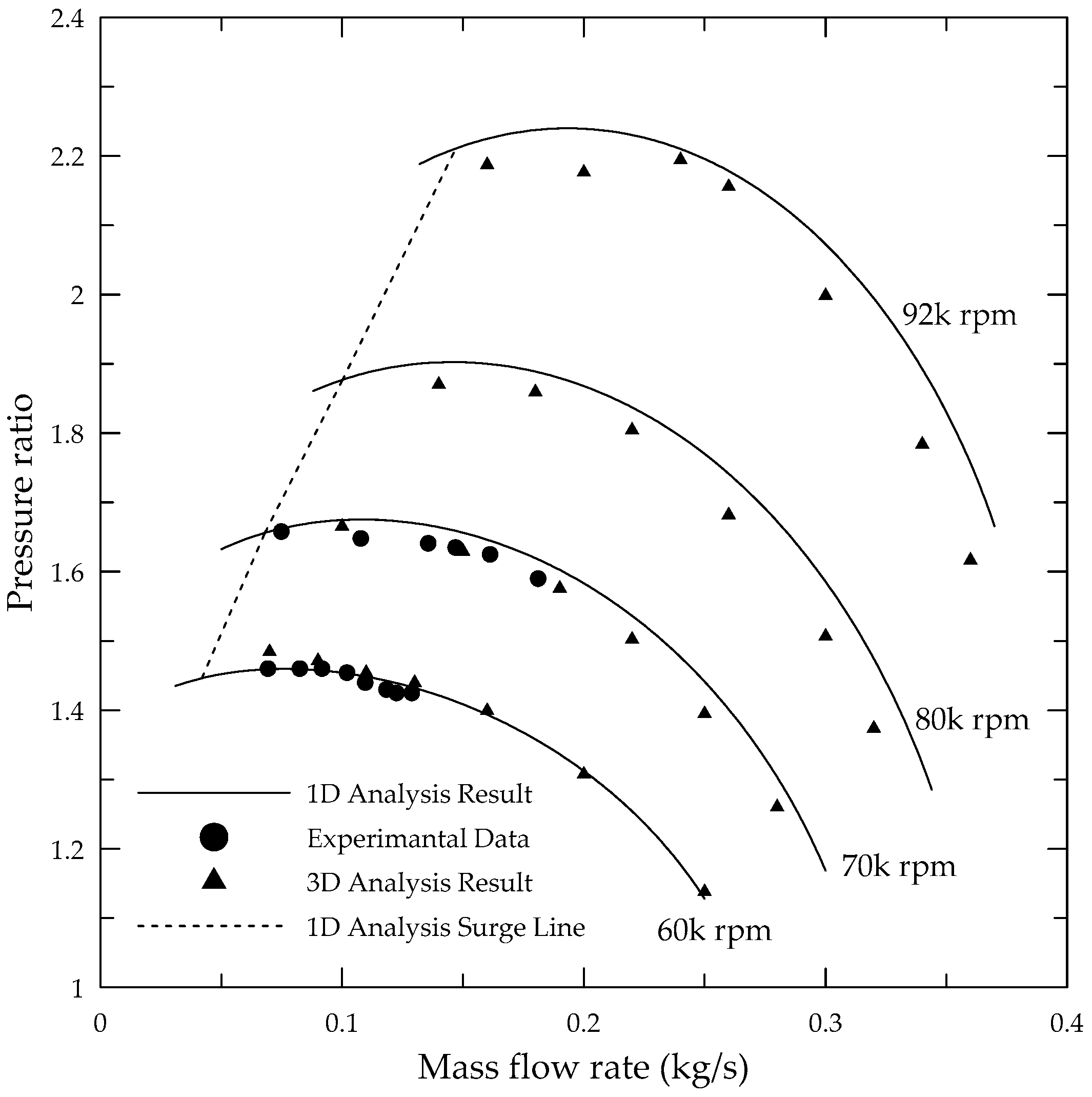
Pressure ratio versus mass flow rate was reported for 60k, 70k, 80k and 92k rpm rotational speeds, as shown in Figure 5. 1D results and 3D model results with available experimental results [36,37] are shown. The results show good agreement in which 3D model results of pressure ratio meet experimental data with negligible error and 1D results were well fitted in lower rotational speeds.

The 1D prediction results show lower accuracy for increasing rotational speed and mass flow rate. The maximum error between the 1D and 3D results was 1.6%, 3.4%, 7.3% and 8.1% respectively in 60k, 70k, 80k and 92k rpm rotational speed, which all occurred in high mass flow rates. This percentage of inaccuracy was acceptable for 1D analysis with respect to overall geometry [32] however, the higher obtained difference at higher rotational speeds was due to the deficiency of 1-D predictive simplified models.

The surge limit line predicted by 1D analysis is also shown in the figure, which was used as a limitation for 3D runs.

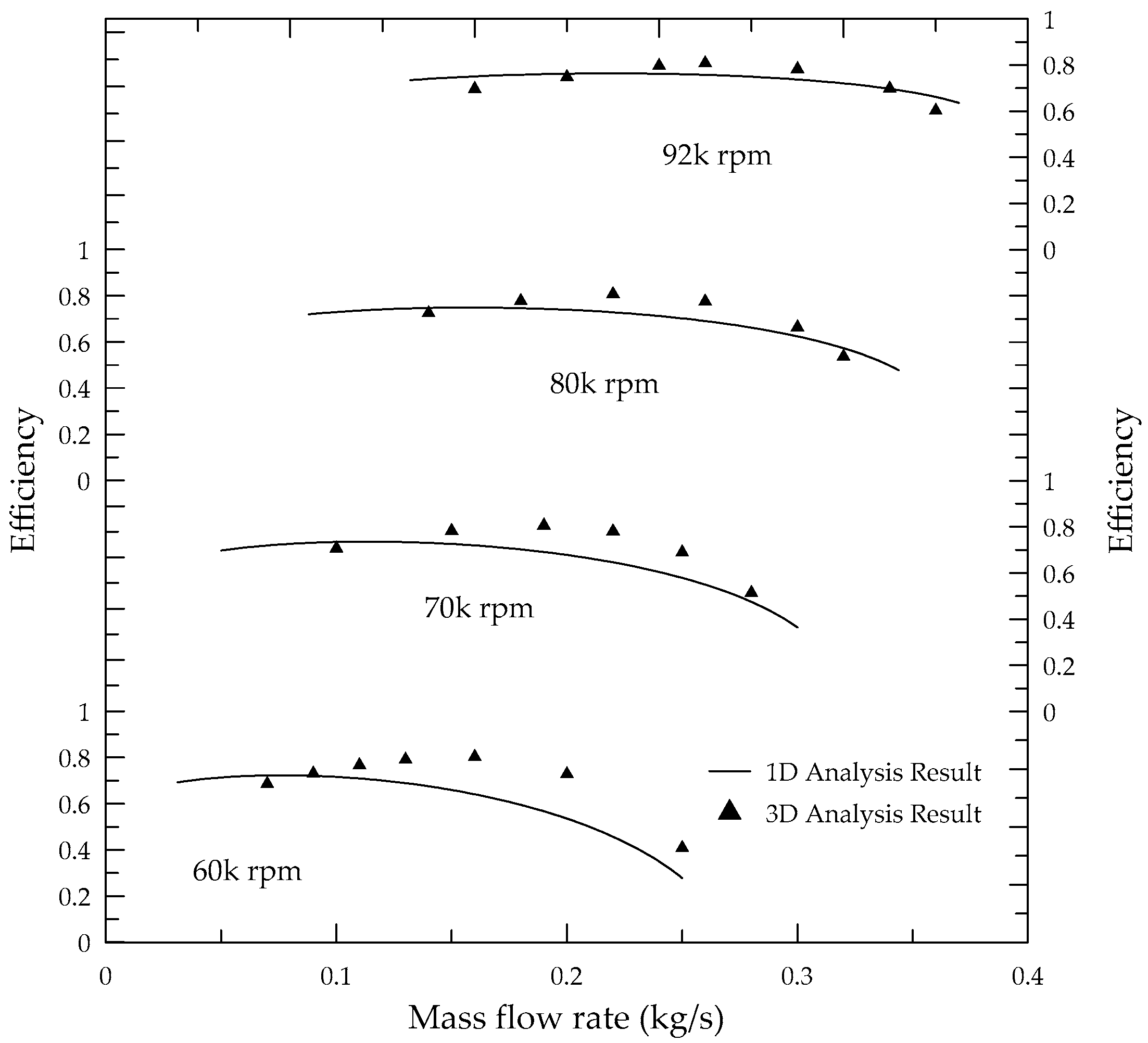
Isentropic efficiency versus mass flow rate is plotted in Figure 6. 1D and 3D numerical results were reported and compared. The differences between 1D and 3D results were limited to below 10% for 80k and 92k rpm rotational speed however for lower rotational speeds the difference increased to about 15% and it seemed 1D procedure predicts the efficiency in low rotational speeds with considerable error. Since the pressure ratio was predicted with negligible error, inaccuracy inherits in the prediction of the stagnation temperature at the discharge regarding Equation (35). 1D loss models except recirculation, clearance and disk friction, did not affect the stagnation temperature of flow based on the predefined correlation [7] whereas in reality and 3D modeling, losses, mainly skin friction (viscous dissipation), affect the temperature of flow. This can be a reason for inaccuracy of predicted efficiency in the lower rotational speeds.

5.2. Design Parameters

Performance characteristics such as pressure ratio and operating range were highly dependent on design parameters, thus, knowing the effect of each design parameter on the overall performance could help the designer to improve the initial design. Furthermore, the share of each loss mechanism clarifies the significance of it, which allows the designer to know the priority of losses to be enhanced during the optimization stages.

The effect of five design parameters including impeller blade height at the outlet (b₂), impeller inlet diameter at the shroud (d_1s), impeller blade angle at the inlet (β_B1), impeller blade angle at the outlet (β_B2) and diffuser diameter at the outlet (d₃) on the compressor pressure ratio was investigated by changing them marginally under and over the design value separately, results are shown through Figure 7, Figure 8, Figure 9, Figure 10 and Figure 11 respectively. Since the 1D analysis pressure ratio result was close to experimental data at 60k rpm, a comparison was carried out at this speed.

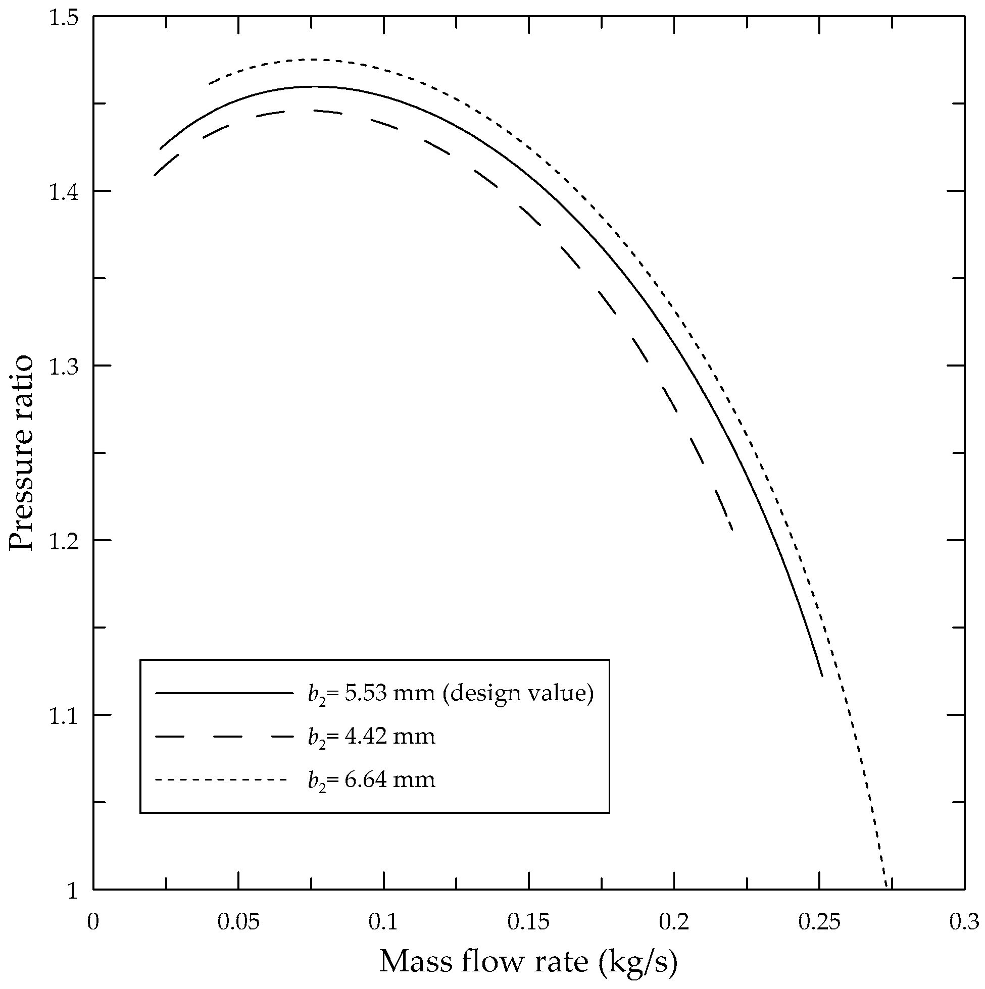
Increasing the impeller blade height at the outlet increases the pressure ratio, due to reducing average velocity in the impeller and reducing the losses consequently, also the compressor operating range shifts toward the larger mass flow rates (Figure 7).

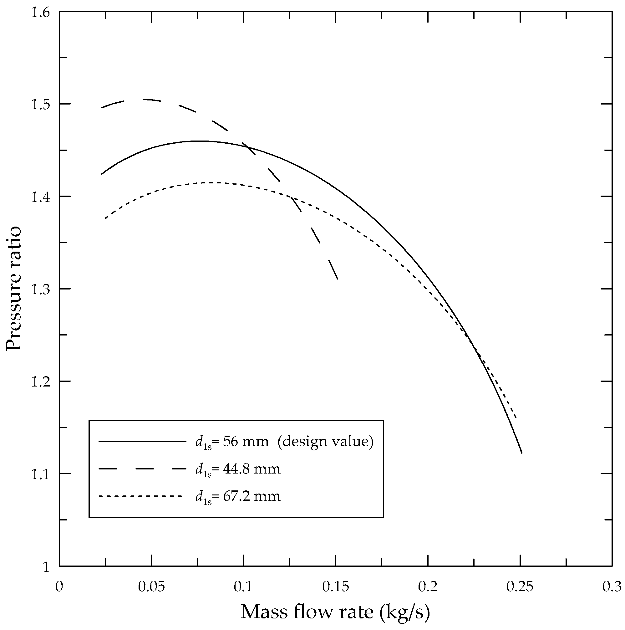
Reducing the impeller inlet diameter at the shroud narrows the impeller inlet area, which makes the average velocity larger in the whole stage. In the case of the current model, the larger velocity increases the pressure ratio significantly at the lower mass flow rates due to the reduction in all losses but it results in the operation range reduction as the impeller passages choke earlier as shown in Figure 8.

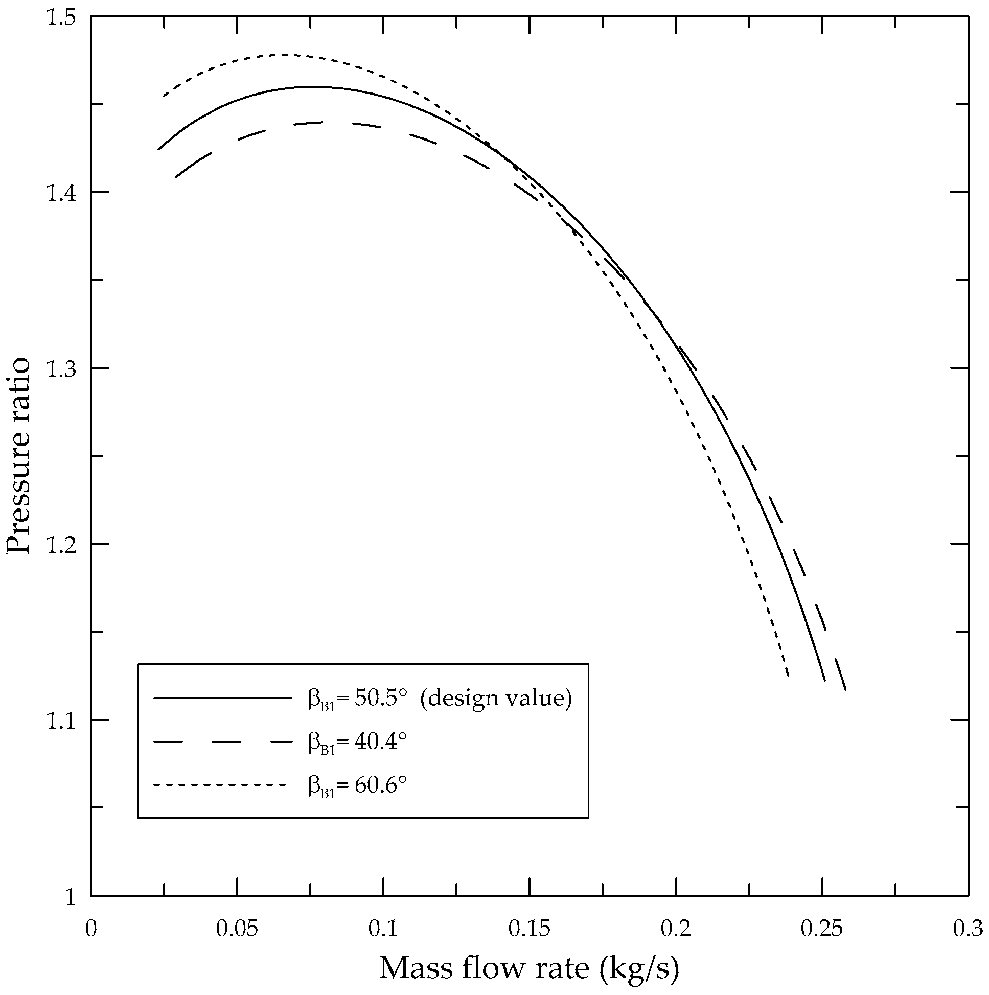
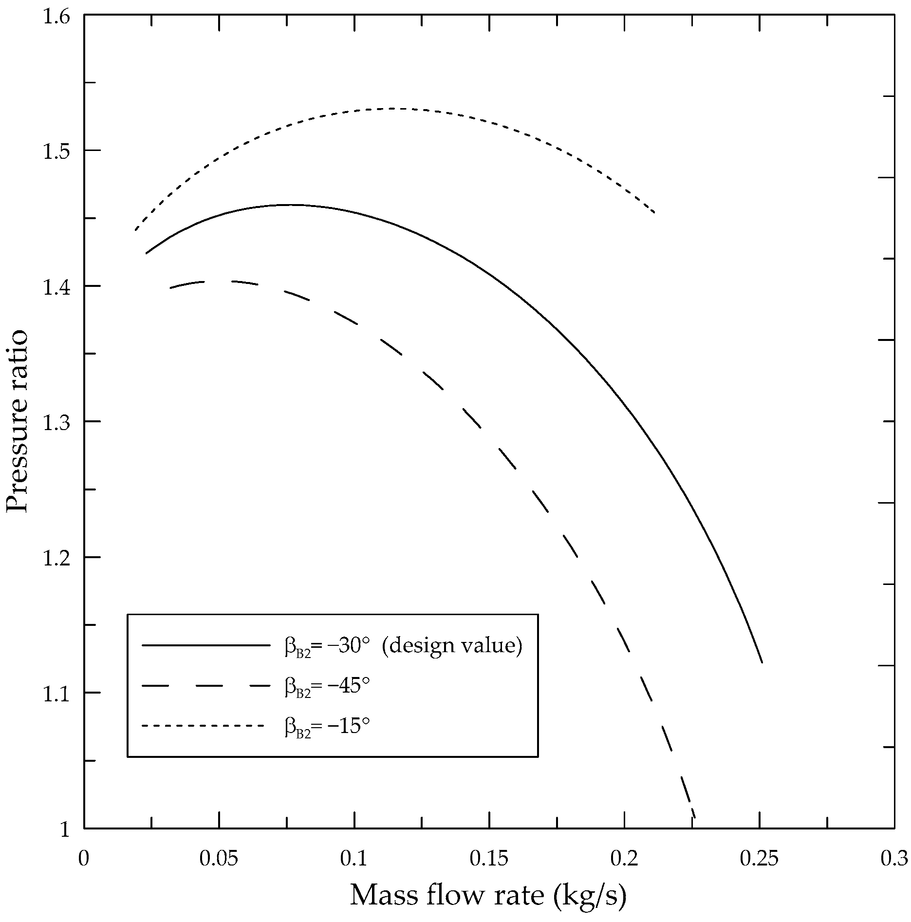
As shown in Figure 9 increasing the impeller blade angle at the inlet increased the pressure ratio around the design point region, which was due to a reduction in the incidence loss. Increasing the blade angle at the outlet increased the pressure ratio as can easily be seen in Figure 10 but it increased the impeller outflow velocity so gas static pressure was low, which is not favorable, also the operation range was decreased.

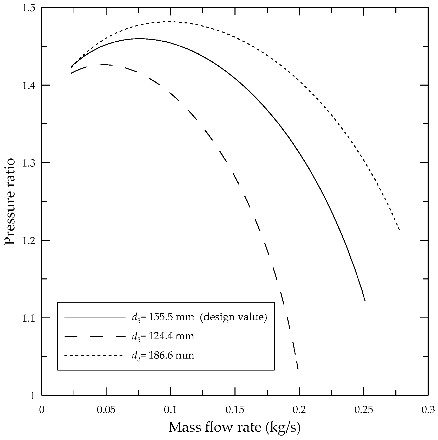
Increasing the diffuser discharge diameter increased the pressure ratio as this recovers more dynamic pressure to static pressure. Although the path of gas in the diffuser became longer causing larger friction loss, diffuser outlet flow velocity decreased, which caused volute and overall loss reduction (Figure 11).

5.3. Loss Impact

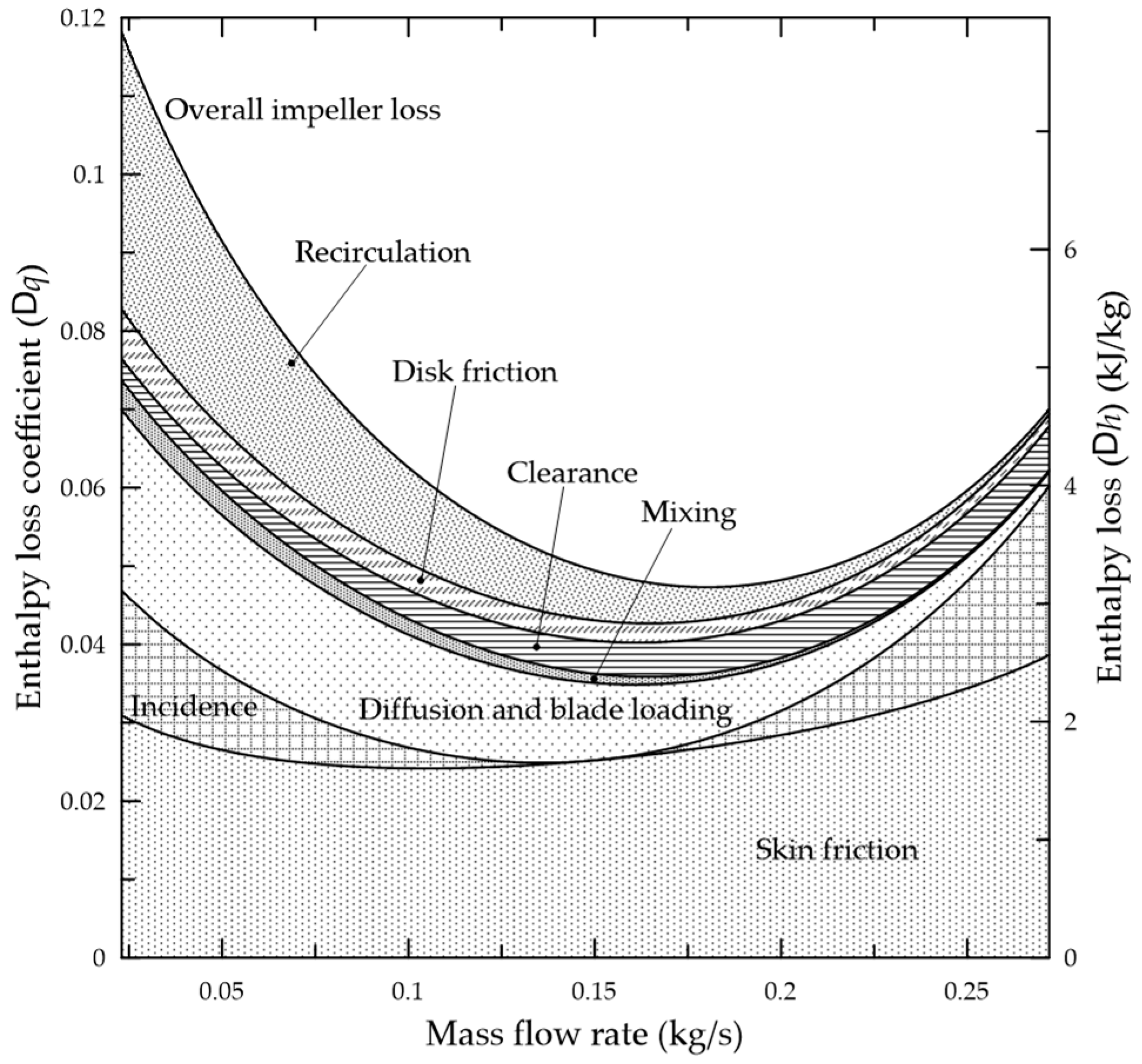
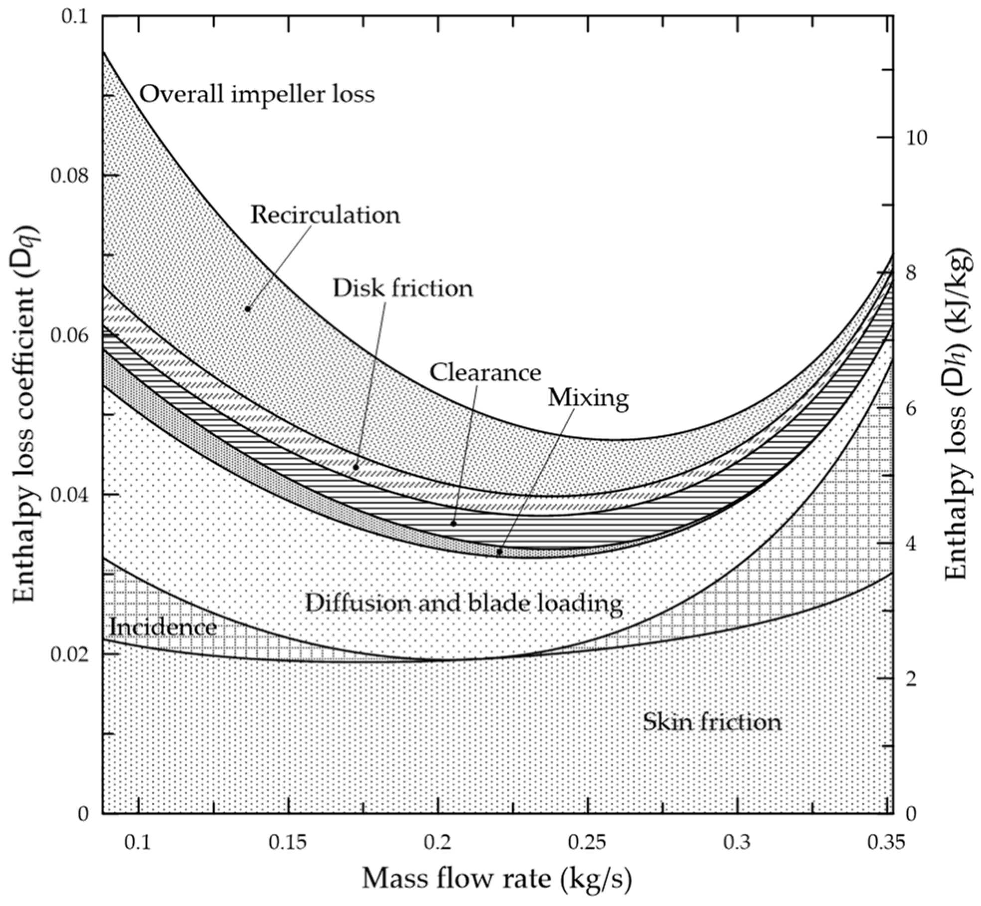
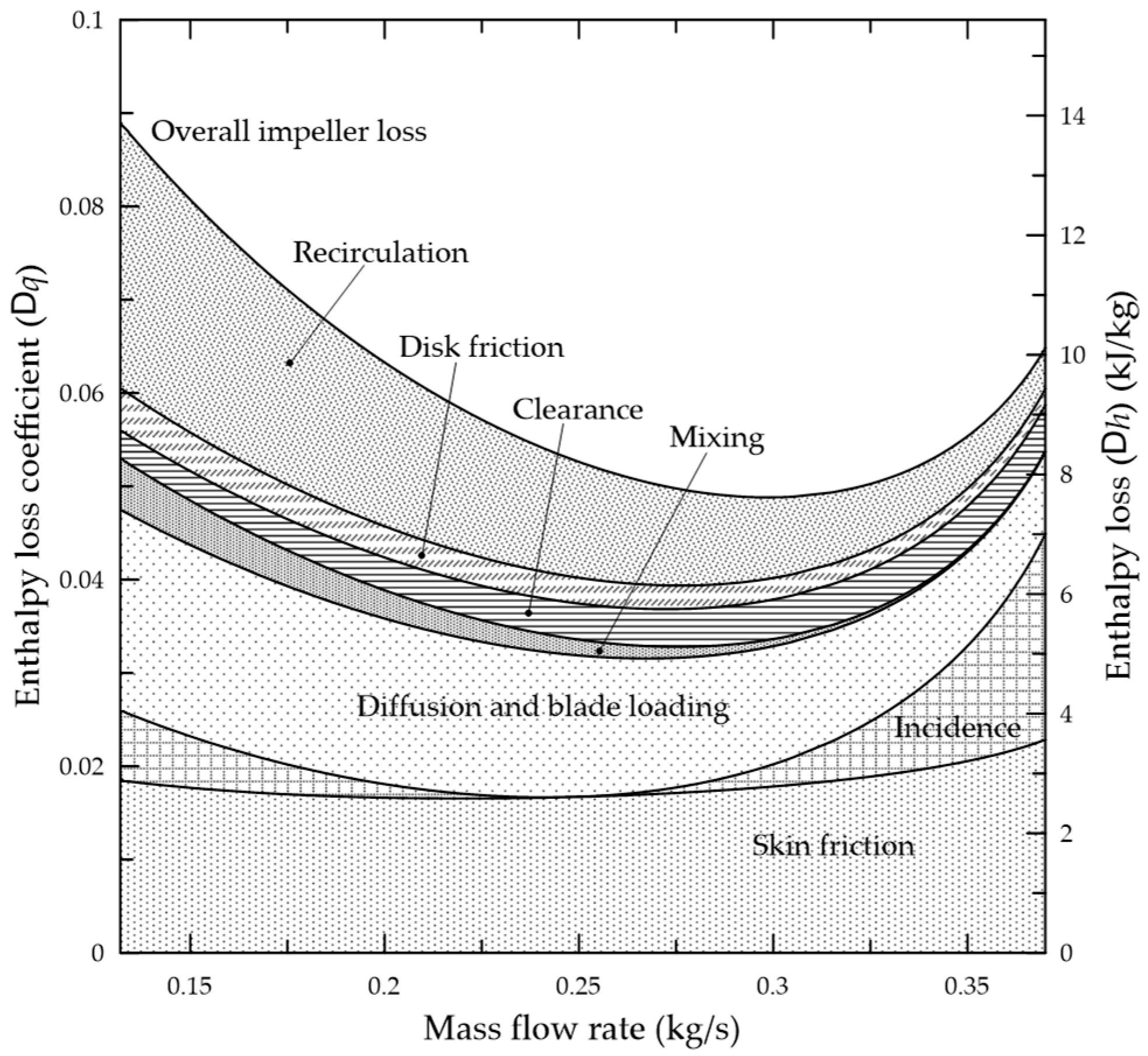
The impact of each loss mechanism on the overall performance of the impeller in the wider operating range of compressor was now investigated. The share of each loss mechanism of the impeller at 60k, 80k and 92k rpm rotational speed is reported through Figure 12, Figure 13 and Figure 14 respectively. As it is shown, skin friction, diffusion and blade loading and recirculation losses were the most important losses with 39%, 23% and 19.5% of total loss respectively in 60k rpm rotational speed. Other losses including clearance, disk friction, incidence and mixing loss with 6%, 5.5%, 4% and 3% of total loss respectively had a lower impact on overall performance.

By increasing rotational speed, the share of skin friction loss decreased as the diffusion and blade loading and recirculation loss share increased. These losses had 29%, 26% and 25.5% share in 80k and 26%, 28% and 27.5% in 92k rpm rotational speeds respectively.

Skin friction loss had a minimum value and increased by increasing the mass flow rate. Increasing mass flow rate caused larger velocities through the impeller passages and resulted in much greater friction loss, while skin friction coefficient decreased in respect of the mass flow rate.

Incidence loss had a minimum in the point that inflow relative angle equaled the blade angle at the impeller entrance and flow entered the impeller smoothly without any sudden change in direction, more or less mass flow caused incidence loss.

Diffusion and blade loading loss decreased as mass flow rate increased, explained by the reducing diffusion factor, D, which means the momentum loss of flow due to boundary layer and secondary flows decreased by increasing stream momentum due to larger relative velocities. Mixing loss also showed a decreasing trend as the wake fraction decreased and flow absolute angle increased by mass flow increase. Clearance loss share was increased in most of the operation range and then declined slightly. Larger flow relative velocity due to higher mass flow rate increased the leakage and hence the clearance loss. Significant reduction in pressure ratio was probably the reason of decreasing leakage flow and the clearance loss in the high mass flow rates.

Disk friction loss share reduces with increasing mass flow according to loss model equation (Equation (18)). Recirculation loss share also reduced in respect of the mass flow. Increasing mass flow caused the impeller outflow to exit straighter, which means the outflow absolute angle increased and the possibility of re-entering of the flow into the impeller would decrease, which reduced the recirculation loss.

6. Conclusions

In this research, the performance of a centrifugal compressor was obtained using 1D mean-line and 3D simulations. Principal loss mechanisms were reviewed and employed to develop a 1D model for one stage centrifugal compressors. A 3D model of the compressor components was created, meshed and solved using a viscous solver with the RANS method.

Total pressure ratio and isentropic efficiency versus mass flow rate for different rotational speeds were used for comparing the 1D model with 3D modeling. Experimental data at two rotational speeds were also implemented for verifying total pressure.

Using a 1D model the effect of the impeller and diffuser geometry on the compressor performance when the high pressure ratio at the design point was of interest also investigated comprehensively and itemized as below:

Impeller blade height at the outlet: Higher value led to higher pressure ratio, lower surge margin, later choke and wider operating range.

Impeller inlet diameter at the shroud: Lower value led to higher pressure ratio, lower surge margin, earlier choke and shorter operating range.

Impeller blade angle at the inlet: Higher value led to higher pressure ratio, earlier choke and shorter operating range.

Impeller blade angle at the outlet: Lower value led to higher pressure ratio, better surge margin, earlier choke and shorter operating range.

Diffuser diameter at the outlet: Higher value led to higher pressure ratio, better surge margin, later choke and wider operating range.

The portion of each loss mechanism in the impeller was studied for different rotational speeds. The results show that the skin friction, diffusion and blade loading and recirculation losses were the most important losses. Other losses including clearance, disk friction, incidence and the mixing loss have lower impact on the overall performance of the compressor.