A Memory-Efficient True-RMS Estimator in a Limited-Resources Hardware

Abstract

More and more human activities are increasingly dependent on the power quality energy they are supplied. In particular, those loads that have an electronic switching mode power supply (SMPS) and microcontrollers or microprocessors are very susceptible to de-energization of the AC line as voltage monitoring takes place on the DC end and may not have enough time to cope with a voltage event involving energy loss. There have been many proposals that analyze power quality or current consumption, even those using limited resources hardware or the classic formulas of discrete root mean square (RMS). In this proposal, an approximation to the problem by means of an RMS value estimator that uses as a base a microcontroller of basic range and low economic cost and algorithms of calculation of very low computational cost that elude complex arithmetic operation to controllers, such as powers or roots, is presented. The results of the experiments to which the proposal was subjected show its ability to provide an estimation of the RMS value of voltage with sufficient precision or an event alarm in less time than the options analyzed. The validation tests and functional comparison of the prototype which were carried out support its viability.

1. Introduction

Reliable and clean electric power conditions many human activities. Electric power is deemed ‘reliable’ if the electric supply is available and dependable. It is also called ‘clean’ if the AC current and voltage waveforms that are supplied essentially fit a sinusoidal wave shape at a frequency of 50 Hz or 60 Hz depending on countries where users live.

Regarding its quality and reliability, electric power is deemed ‘computer grade’ if it is specially conditioned and controlled ultra-clean electric power. By contrast, ‘dirty’ electric power is characterized by a significant distorted waveform which contains undesirable components like pulses, off-frequency sinusoidal waves, and other undesirable deviations from the sinusoidal desired waveform. These components can be transient events, they can repeat periodically at AC mains frequency, or they can cycle at higher or lower frequencies related to that, i.e., harmonic or subharmonic components [1].

Outages (i.e., power interruptions, including blackouts) can also cause serious consequences. Computer data can be lost; a shaft on a large, idle, rotary machine can bow or sag; molten metal can solidify; heating systems can shut down; protection systems can fail; a hospital’s life-support equipment can become inoperative; and a chemical processing plant can experience runaway reactions.

Dirty power, steady-state undervoltages (brownouts) and overvoltages can lead to electrical and mechanical equipment damage.

Power quality and reliability (PQR) problems affecting the voltage in quantity or magnitude that occur in home or business facilities involve transients, sags, swells, surges, outages, harmonics, and impulses [2]. Short-term power quality disturbances include dropouts, sags, and swells. Dropouts are momentary power losses typically occurring within one electrical cycle. Sags are depletions of power caused when heavy loads start. Swells are power surges caused by sudden load disconnects. Sags and swells are typically seen as voltage changes lasting 2.5 s (150 cycles for a 60 Hz system) or less upon sudden changes in power demand.

They can disrupt sensitive loads or cause harm to installed equipment. Electronic equipment especially is highly susceptible to all three problems.

Before electronic loads were common, simple surge arresters, power supply transfer switchgear, and voltage regulators assisted most equipment and systems to tolerate common power problems and perform adequately. However, electronic loads are increasing and consume more than half the power generation capacity in the developed world. These loads are sensitive to power quality problems. Furthermore, in much of the electronic circuitry in use today, electronic power supplies with switching frequencies as high as 200 kHz have replaced older, linear (sinusoidal) power supplies. Switch-mode power supplies lower power quality. Today, while the miniaturization of modern electronic devices makes reliable, clean power even more crucial, these same electronic devices have become a major contributor to the dirty power problem.

Typically, power-conditioning equipment combines voltage regulation with power system isolation and shielding. Uninterruptible power supply (UPS) systems are generally an excellent way to control power distortions, but their primary purpose is to improve power reliability, not to clean poor power quality. Among those which exist there are currently available many solutions to voltage regulation [3,4]. Among them, UPS and AC/DC power factor correction (PFC) converters with universal voltage supply range and equipped with surge suppressors, which very often include a power digital manager module at the DC side and frequently may be found in very sensitive domestic electronic equipment. However, electrical appliances are one of the most complex sets in the Smart Grid definition of sensitive equipment; there also are adjustable and sheddable loads [5] managed with different strategies.

Electric power supply problems are inappropriately considered service quality problems and the sole responsibility of utility companies. However, a user’s distribution circuit arrangement, system, and equipment can contaminate the power supply and cause power supply interruptions. Thus, utilities, equipment manufacturers and system designers all share responsibility for power supply conditions.

Those effects are less critical in appliances powered by switching mode power supply (SMPS) where the front side power converter filters and smooths most of the voltage level and frequency electrical disturbances within the range of the universal input supply range [6]. However, power abnormalities and waveform distortions cause control, data processing, and diagnostic systems to operate erratically and can lead to faults in microcontrollers and, consequently, operation downtime and process rejections with variable operating costs.

Furthermore, electronic control equipment needs fast and reliable voltage brownout detectors [5,7] in order to equip the adequate protection or compensation strategies or to detect voltage sags as fast as possible and trigger adequate alarm or control signals [8].

Finally, the Smart Energy Profile 2 (SEP 2) standard promoted by the Consortium for Smart Energy Profile 2 Interoperability (CSEP) enables management and control of smart grid devices in the home [9]. In this scenario, a fast and accurate RMS value measurement or estimator algorithm for any electrical variable which could be easily embedded in either home area network metering devices or smart appliances is also needed. Wider ARMs and sensor networks cannot be avoided either.

If the de-energizing process were only detected when the SMPS outlet was out of range, the affected intelligent load would not be able to adapt its run mode to deal with it.

Every PQR event may be defined according to the relationship between its residual voltage level and duration, as reflected in the standards EN 50160 [10] and IEEE 1159-2009 [11].

Moreover, the International Working Group (JWG) C4.110, sponsored by CIGRE (the International Council on Large Electric Systems), CIRED (the International Conference on Electricity Distribution), and UIE (the International Union for Electricity applications), has established a description of the different properties and characteristics of voltage dips based on dividing a dip into transition segments and event segments [12].

This works firstly aims to the automatic in advance detection of de-energizing dip, brownout, or outage events related to the AC voltage at the supply inlet by means of its phasor module measurement instead of monitoring the converter DC outlet.

One of the mean advantages of using micro-controlled SMPS is the monitoring of the power converter that leads to a supervisory function that produces an idle state or a soft switch-off if necessary. Many of those systems are based on the DC voltage level in the DC bus at the converter outlet.

This means that if a DC undervoltage occurs at that point, the output filter capacitor had been supplied all the energy it had stored for correct functionality and no operational return point could be achieved because of the recharging time gap needed to re-energize it. Consequently, the microcontroller faults and the appliance program resets.

However, the good news is that the AC mains can degrade their power quality several cycles before the power converter becomes de-energized.

A brief overview of the state of the art (SoA) on signal quality metering using microcontrollers shows the use of a widespread variety of hardware provided with different resource levels.

There are diverse approaches to the measurement of the quality of the electrical signal. Some of these use the RMS value of the signal and others use other parameters on which they carry out more complex transformations like the wavelet transform. Some of them are also implemented using limited resources systems, as described in [13], which employs a limited resources system based on an ATmega 328P microcontroller (Microchip, Chandler, AZ, USA). This system measures voltage, current, active power, and power factor over various loads and wirelessly transmits them to the main brain for processing. Voltage and RMS current are calculated to evaluate the energy consumption in each load, but it does not detect voltage drops. In [14] the ESP8266 module is used for THDi (Current Total Harmonic Distortion) via FFT (the Fast Fourier Transform), and the current RMS value for each load is given via the RMS method. The values of these parameters are transmitted to a server and implemented through a Raspberry Pi, using the MQTT (Message Queuing Telemetry Transport) protocol so that the user can monitor the energy quality signal and know the electrical faults of a load or the network. This monitoring system has the disadvantage of not being able to detect faults in real time. In [15] the power quality parameters of a single phase are measured and the arc-fault series are sensed, but the voltage drops are not able to be detected in real time. It uses a limited resources Microchip (Chandler, AZ, USA) dsPic33 processor to calculate the wavelet transform and the pass fundamental frequency using the zero-crossing technique, as well as RMS values and power. In [16] the V_rms for a specific number of signal periods is calculated, meaning it can detect neither voltage drops nor surges in real time. Its objective is to achieve an accuracy of 0.1% in the measurement of the RMS value with an analog-to-digital converter (ADC) of 10 bits so it is constrained to use the oversampling technique and therefore does not optimize the time of calculation to provide an RMS value. The system uses a single limited resources, low power CMOS 8-bit microcontroller based on an AVR-enhanced RISC (reduced instruction set computer) architecture.

In [17] some signal quality parameters such as V_rms, I_rms, active power, power factor, and THDi are measured and sent through the power line to a concentrator that makes decisions based on the consumption strategy adopted by the user. Therefore, it does not detect voltage drops. An STM32F407VG microcontroller is used to acquire and process the signals, and send them via a PLC (Power Line Communications) modem to a Raspberry Pi, model B.

In [18] the system uses the wavelet transform to detect voltage drops. It uses a sampling time of 156 μs, and although the calculation time is less than the acquisition time (32 μs), the final time needed to detect the voltage drop is much greater, on the order of 5 ms, since it needs to acquire 32 samples. This system uses a DSPIC processor.

The second aim of this work is to check the feasibility of a proposal of an RMS estimator built using limited resources hardware and to validate its reliability and accuracy to prove that even limited resources microcontrollers which are not intended for arithmetic functions are able to perform and to achieve an estimation capable of providing as fast as possible an RMS phasor module value to be used in a voltage control loop or in a de-energizing alarm system.

Section 2 describes the fundamentals of the RMS calculation. Section 3 approaches the methodology used in this proposal from the system functional blocks to the algorithm implementation including low computational complex arithmetic to estimate the phasor module. The paper finishes with the description of the experiments performed and the consequent results in Section 4 from which the conclusions are drawn in Section 5, where future work is additionally presented.

2. Backgrounding on Root Mean Square Value Calculation

2.1. Discrete RMS Value Determination

The most common way to describe or analyze power quality events is by the measurement of the RMS value of voltage or current. According to [19], the RMS value of an electrical magnitude (e.g., voltage) is determined by the formula:

$$V_{rms}=\sqrt{\frac{1}{T}{{\displaystyle \int }}_0^T{v}^2\left(t\right)\mathrm{d}t}$$

(1)

The discretization of this expression results in [13]

$$V_{rms}=\sqrt{\frac{1}{2^N}{\displaystyle \sum }_{n=1}^N{v}_n^2}$$

(2)

RMS values can be computed continuously whether they are updated each time a new sample is obtained but generally these values are updated with a certain time interval (each cycle or half cycle) in a discrete mode [20]. The IEC standard [19] proposes the U_rms(1/2) discrete measurement method for determining the voltage level during the event.

From the point of view of a customer, the IEC 61000-4-30:2015 standard [19] characterizes a sag/swell at the supply line by means of its duration and remaining voltage. The most common procedure for measuring this minimum/maximum voltage value during the event is the voltage RMS calculation described above. Once this value is measured, the event duration may be determined by comparing this value with the established threshold and hysteresis levels.

On the one hand, the RMS method is simple, well known, and easy to implement. On the other hand, the limitations in the use of RMS values in power quality analysis from the point of view of the IEC standard have been clearly overviewed [21,22]. In a single-phase, the major drawbacks that affect both the performance feasibility and the accuracy of results are:

• the dependency on the window length and the time interval for updating the values; the longer the measuring window length the less correct the RMS value estimation for short duration and less severe voltage events
• the dependency on the starting event point-on-wave for calculating the RMS value faster or slower
• the commonly unpredictable large number of processing steps that complex operations like squares or squared roots need, which determines a faster processor clock frequency to avoid sampling lagging or processing gap overtaking.

As a consequence, limited performance in the detection of voltage events and in the estimation of their magnitude and duration is produced.

2.2. Using the Moving Window to Evaluate the Voltage Magnitude

In contrast to the U_rms(1/2) discrete measurement, in the RMS voltage magnitude evaluation by means of a moving window [23,24] the values are continuously calculated from the input voltage samples. This method expresses the energy content of the signal and provides a convenient measure of the magnitude evolution. Assuming that the window contains N samples per evaluated signal period, the RMS value at sampling instant k can be calculated by:

$$V_{rms}\left[k\right]=\sqrt{\frac{1}{N}{\displaystyle \sum }_{n=1}^N{v}_n{\left[k\right]}^2}$$

(3)

Thus, the RMS value can be computed each time a new sample is obtained, which requires a large size/amount of data memory if these data have to be stored. In the U_rms(1/2) method, the values are updated each half cycle of the supply signal, meaning the required memory is significantly reduced. The discrete function that illustrates this evaluation method according to Equation (3) is shown in Figure 1. The N-values length data vector used in this calculation is completely refreshed after N samples to prevent buffer overflow.

The discretizing of the supply signal relies on several methods for sampling:

• Zero-cross synchronized sampling [25], where the electrical signal’s zero-across synchronous detection is equal to synchronous sampling with an invariable interval. This method has no error of measurement and only presents errors related to the sampling process or the analog to digital conversion. This synchronous sampling error must be taken into account when sampling non-sine waves. An extension of this method using oversampling is used in [25] in order to measure true RMS values under harmonic conditions.
• Quasi-synchronous sampling [25]. This means that the alternative signal is discretized as a zero-cross synchronized sampling sequence after low-pass filtering the supply signal. The associated errors involve power calculation due to the displacement angle introduced during the filtering process.
• Non-synchronous sampling used in [26] for true RMS measurement based on the calculation of cycle double-end sampling values.

3. Methodological Approach

As stated above, sensitive electronic equipment needs voltage dip detection algorithms which are as fast and reliable as possible in order to become immune to this type of perturbation [27]. The IEC 61000-4-30 U_rms(1/2) determination is not fast enough to achieve this critical requirement; this is, in fact, not its purpose. A simple comparative simulation study was performed in PSIM 11, updating [28], to compare how these aforementioned methods result in an RMS voltage magnitude value, with the results shown in Figure 2. Here, the response time of several sampling rate continuous RMS calculations, a supply period discrete RMS calculation, and U_rms(1/2) for a voltage signal (Vs) are compared. The significant differences between the two compared methods may be easily checked: the moving window method depicted in the traces is labeled as VCrms_x for four, eight, and 16 samples per half a period, respectively, and the IEC method presented in the traces is named VDrms_1T and Urms1_2_6100_4_30.

As stated before, the main objective of our proposal is to follow the changes in the voltage magnitude as closely as possible during the sag/swell event. The more instant voltage values considered or employed in a window, the closer the actual RMS value is [17,18].

3.1. HW Proposal for an RMS Evaluator Prototype

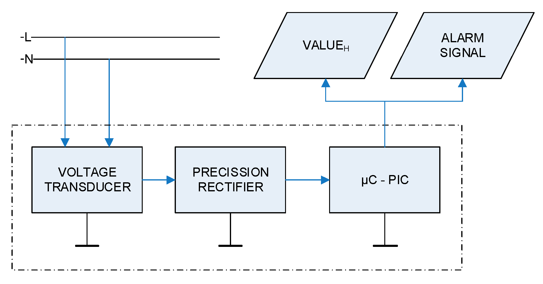
The aim of this work is to propose a memory-efficient algorithm for metering the RMS voltage that runs on limited resources hardware. The proposed and built meter has the block diagram described below (Figure 3).

The voltage transducer block was based on an LEM^® LV-25xx (LEM^®, Milwaukee, WI, USA) [29] circuit that carries out galvanic isolation and scaling functions. Passive element values in its connection circuit were chosen for the nominal supply line voltage. A voltage transducer block is used to adapt the signal amplitude to the microcontroller input range. Once the level has been scaled, the bipolar signal is converted to a unipolar one with a general-purpose precision rectifier.

The precision rectifier is the standard full wave version of this function built with limited resources general-purpose operational amplifiers and standard diodes and resistors. This block provides the absolute value of the scaled supply signal and adapts the signal to be measured to the microcontroller ADC range. So far, nothing new has been set in practice.

The estimator proposed in this paper was built in a general-purpose limited resources 8─bit arithmetic logic unit (ALU) PIC that included five multiplexed 10-bit ADCs.

3.2. Fitting the Main Program in the Microcontroller: HW/FW Limitations

The main program flow diagram implemented in the PIC is shown in Figure 4. Note that the first operation to be performed by the main function was to create the look-up-table (LUT) with the set of voltage values and their respective squared values according to the estimation range, as explained in Section 3.3 below.

The selected microcontroller block was a Microchip^® 18Fxx2 PIC [30] that performs the following functions:

• Signal sampling. In accordance with the Nyquist theorem, the sampling frequency must be more than twice the signal frequency in order to avoid the aliasing effect, which has been established with a synchronous sampling frequency of 800 Hz that provides an 8-sample vector per rectified scaled signal period.
• Analog to digital conversion is performed in a 10-bit ADC port.
• Zero-crossing synchronization mechanism.
• RMS voltage measure core function, which is described in a specific chapter.
• The RMS voltage value or the undervoltage alarm sending to an output port.

3.3. Selecting the RMS algorithm for Voltage Estimation

As stated above, limiting the time for a square or a squared root calculation may be the Achilles heel in this step, due to both operation spend for an a priori unknown number of processing steps, i.e., squaring a number might be highly dependent on the number size, and rooting another one could require many steps before the result converges. For instance, the time gap used to perform the Babylonian algorithm for square rooting is highly dependent on convergence speed and this dependence becomes uncertainty.

Given that our purpose is to obtain the most accurate possible value in the least time possible with the hardware employed, the focus of this procedure was on modifying and simplifying the RMS value calculation algorithm.

All the data were declared as unsigned integers.

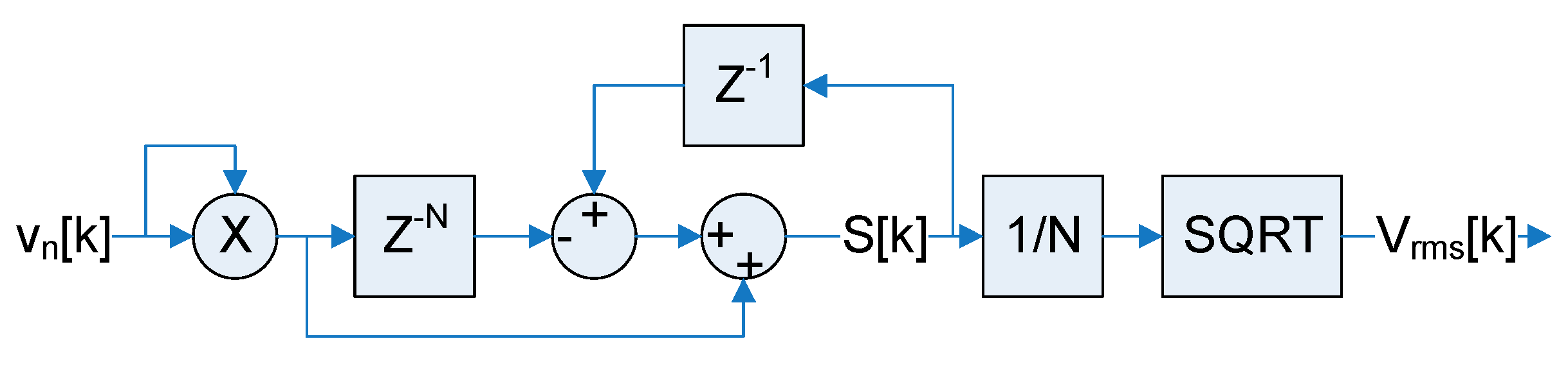
The selected method for voltage value or event detection is an evolution of voltage RMS magnitude continuous evaluation using a moving window. As in the original method, the supply signal is discretized and processed using Equation (3) being rewritten in the following way:

$$V_{rms}\left[k\right]=\sqrt{{\displaystyle \sum }_{n=1}^N{\frac{v_n\left[k\right]}{N}}^2}$$

(4)

Using this method, the squared values of the sampled vector are divided by the vector length prior to the summation. Hence, by choosing an 8-data vector length, the instruction of dividing an integer by eight becomes a faster operation than the division by a non-power of two. In such a way, the 16-bit size of the data will not be overflown by the results and, therefore, will optimize their size. Thus, the discrete time function described above in Figure 1 was able to be restructured as shown in Figure 5.

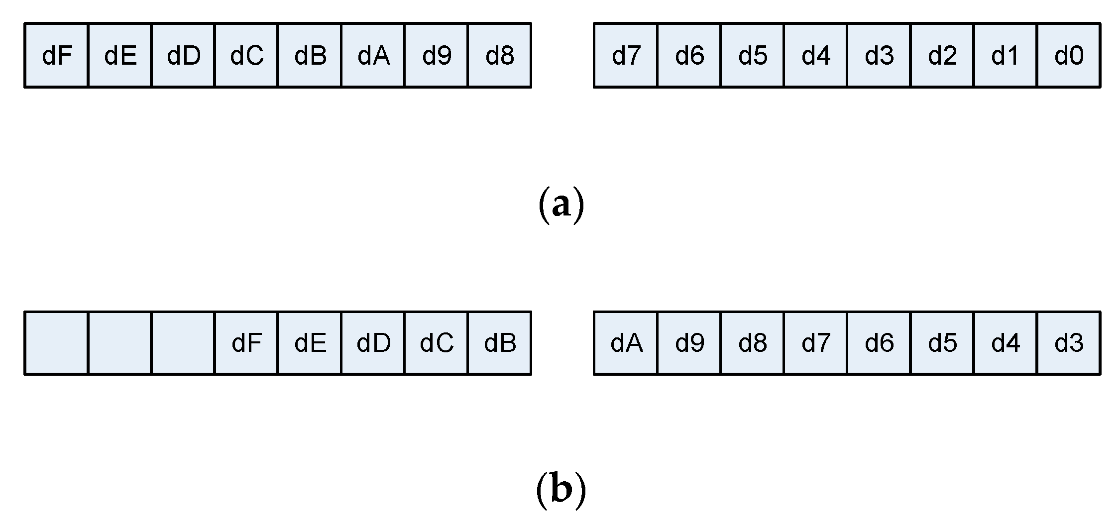
Working with powers of two values allows simplifying all the calculus to be done as well. Thus, only the eight most significant bits (MSBs) of the 10-bit data from the ADC were considered, as displayed in Figure 6. Otherwise, the squared value of a 10-bit datum would be that of a 20-bit one, with the result that the microcontroller’s basic data size would be exceeded and there would be a need for a more than double register size register to define the result.

The RMS-calculation algorithm starts using these eight MSBs from the ADC output (Figure 7a) as the datum’s index pointer of its squared value (Figure 7b) stored in a kind of lookup table. This squared datum is 16-bits long.

Any additional operation would surpass the established limit of 16 bits, so if it was divided by eight, the data vector length, prior to the summation the result should fit within a 13-bit value. This division is displayed in Figure 8. Consequently, the sum of eight 13-bit terms will never exceed a 16-bit size.

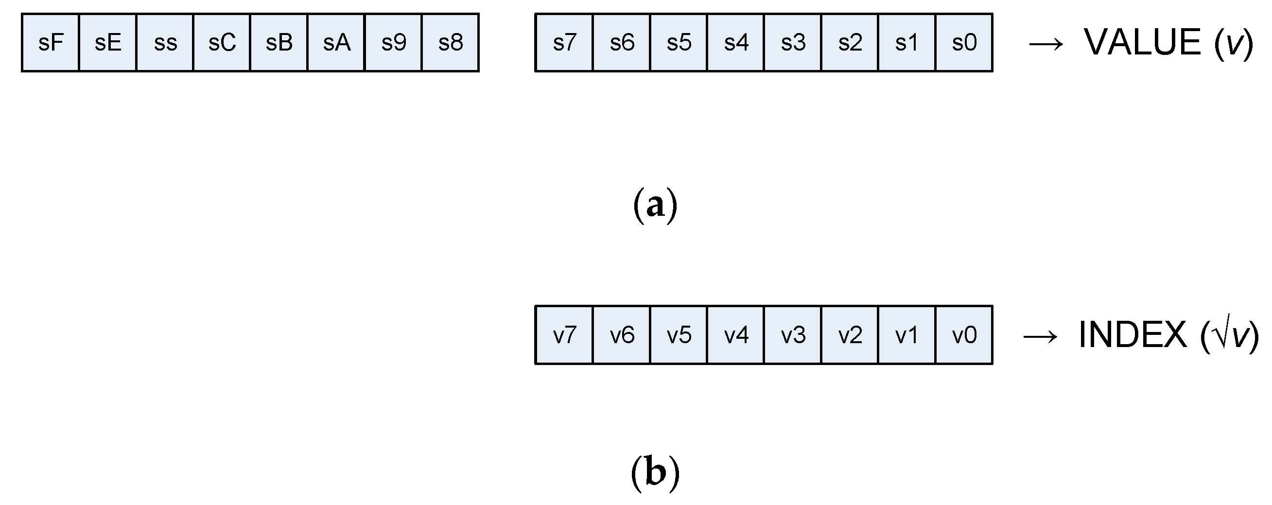
Once the data vector has been summed, the square root is as easy as finding the address of the data vector that matches or is close to the sum result. Both the data and the summation sizes are depicted in Figure 9.

The selected method used to find the square root value of the summation is the bisection method, which is also called the binary search method. This method allows for the obtaining of a valid solution in a maximum of eight, which is the solution length in bits, comparison steps and, as a consequence, the solution can be obtained in a very short time with a very low computational cost. Figure 10 shows the relationship between the summation value and its position index to get the solution.

This solution can be inputted into a communication port, compared to an alarm threshold level, or used as an input argument in other functions, such as a discretized voltage control loop.

The LUT for the RMS calculation algorithm is illustrated in Figure 11.

Finally, the relationship between the proposed moving window function for RMS evaluation and the register size can be clearly seen in Figure 12.

All the processes in the algorithm can be easily written in assembly PIC code or C/C++ language, minimizing and optimizing the program size and its execution time.

4. Performed Experiments

A set of different experiments were carried out with the prototype under testing in order to achieve its overall performance. For that purpose, static and dynamic tests were designed and the obtained results may indicate the proposal’s abilities.

Firstly, on the one hand, for these experiments, the voltage transducer block scaling factor was established in 1:100 to fit the desired measuring range upper limit to 500 V and adapt it to the microcontroller ADC input range, which was set as up to 5 V. This upper limit was set because it is just over 150% of the supply voltage peak value, i.e.:

$$1.5·\sqrt{2}·230+2\%$$

On the other hand, there were only 8 bits considered from the 10 ADC output. Thus, the ADC resolution was set to 19.6078 mV per step, i.e., each bit in the RMS value corresponded to 1.96 volts with the referred scaling factor.

In the second stage, the speed of event detection capability and a performing algorithm evaluation regarding some measured data series were carried out.

Finally, a comparison experience was undertaken. A similar system was built with another limited resources microcontroller running a standard RMS basic algorithm with a 1 kHz sampling frequency in order to highlight its measuring uncertainty with respect to our proposal.

All the steps described above are covered in the following subsections.

4.1. Checking the Accuracy

To trial the accuracy of the proposed algorithm, the RMS estimator was correlated with the TRMS voltmeter of a Fluke ScopeMeter^® (Fluke^®, Everett, WA, USA) series 120 in order to check its accuracy. A set of steady-state metering tests were implemented for a series of supply line voltages from, approximately, 0.1 pu to 1.25 pu provided by an autotransformer in the experiment topology shown in Figure 13.

The correlation results are displayed in Figure 14.

Note in Figure 14 that the absolute difference between the maximum and minimum values provided by this proposal is the discretization step (1.96 V) in all cases and the relative error quickly reduces as the gap between the actual value and the estimation limits remains limited while the value of the phasor module increases. Figure 15 depicts the relative error for both the maximum and the minimum phasor module value estimations regarding the real objective value measured with the reference true-RMS digital multimeter.

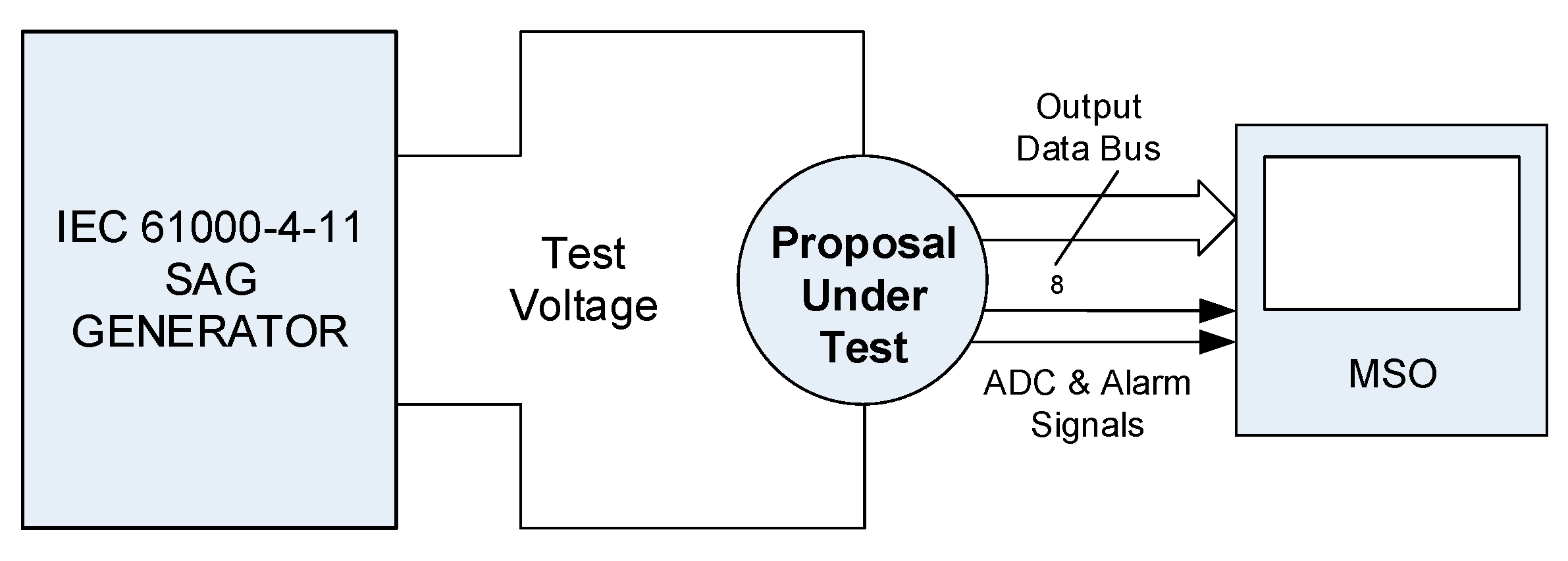
4.2. Dynamic Response: Event detection and Present Value Estimation

Once the meter was characterized and its accuracy tested, more experiments were carried out to check the meter dynamic response. The circuit used for this set of tests is shown in Figure 16. The worst case analyzed, a 0.7 pu sag beginning at the zero-crossing supply signal, resulted in a time of 6 ms for the sag detection (a level below the 90% of the nominal value) and 8 ms for a valid remaining voltage metering, as shown in Figure 17.

Note that due to the event which took place at the null instant voltage value (signal zero crossing), the first value capable of modifying the summation is taken in the following sample, 1.25 ms later).

4.3. Comparing the Proposed Estimator Accuracy to Standard Measuring Methods

Once the initial accuracy test was successfully checked under lab conditions, several validation processes used to prove its capability for detecting de-energizing events with sets of captured field data were performed.

First, registered data sets from AC mains in home appliances were analyzed using the algorithm used in [31]. Herein, in contrast to what was stated in the previous subsection, the experiment omitted zero crossing synchronization but achieved sufficient accuracy.

In the second stage, processing data from a 3-phase substation outlet were contrasted with data obtained from the already installed instrumentation at the facility.

In Figure 18a the time series of the 3-ph voltages with a clear brownout are shown. The measured data from a 96 sample per period double-precision data vector moving window from a DSP (digital signal processor) metering device (grey color and the legend ‘VxMW48′), lines RMS values obtained using the IEC 61000-4-30:2015 method for half a period (orange color and the legend ‘Vx61k4-30′), and the data provided by this proposal (blue color and the legend ‘Proposal’) are depicted in Figure 18b–d, respectively, for each AC phase.

4.4. Contrast Experiment: Expanding the Samples Vector and Employing the Whole Math Function Library

To perform this experiment, a general purpose ATmega328P microcontroller-based prototype, as given in [22], was built and configured with a clock frequency of 16 MHz. The selected sampling frequency was 1 kHz, i.e., a 20 samples per AC voltage signal period, and the programmed procedure fit what is described in Figure 1 and in Equation (3).

The contrasting demonstration was limited to the dynamic response since the static accuracy had been verified as being as good as that from the proposed system. As has been mentioned in previous sections, no zero-crossing synchronization was performed in this experiment.

Of the set of experiments carried out, the one corresponding to a sag of 25% is shown. The depicted screens in Figure 19 represent the two extreme cases recorded within this. In this figure, the blue trace corresponds to an active low alarm related to surpassing the 10% undervoltage limit.

Note that the shortest recorded time to reveal a 0.75 pu sag (Figure 19a) is pretty close to our proposal, though the longest one (Figure 19b) triples ours. This is due to the uncertainty in terms of duration both in the second power and in the square root operations.

5. Conclusions and Future Work

In this paper, an RMS voltage estimator that eludes the inherent uncertainty of complex arithmetic operations related to the discretized RMS algorithm has been presented.

Even though there are more accurate and faster methodologies present in the literature, the one proposed in this paper is built using limited resources hardware with a high-efficiency program which minimizes the system requirements and prevents data memory overflow. Therefore, the phasor module estimator presented here limits its response time for providing a valid estimation and it can be implemented in simple microcontrollers that do not have high-performance arithmetic units or specific resources for digital signal processing. Its ability to operate as either a sag/swell detector, a true RMS meter in a protective alarm or idling system, or at a not too demanding voltage loop of a regulator has been assessed and verified by comparing its performance to a low-cost embedded system based on an ATmega328p microcontroller, one of the most basic of those provided by the company Microchip.

The proposal aims in the near future to carry out its implementation in a very low-cost FPGA (field-programmable gate array) that only has basic logical resources such as LUTs, adders, flip-flop, and embedded block RAM, etc., such as, for example, the iCE40 LP/HX/LM family and the integration of voltage and current phasors estimation on a single device. This would allow for the embedding of this feature into a smart home appliance.