Degradation Rate Location Dependency of Photovoltaic Systems

Abstract

A main challenge towards ensuring improved lifetime performance and reduction of financial risks of photovoltaic (PV) technologies remains the accurate degradation quantification of field systems and the dependency of this performance loss rate to climatic conditions. The purpose of this study is to address these technological issues by presenting a unified methodology for accurately calculating the degradation rate ($R_D$) of PV systems and provide evidence that degradation mechanisms are location dependent. The method followed included the application of data inference and time series analytics, in the scope of comparing the long-term $R_D$ of different crystalline Silicon (c-Si) PV systems, installed at different climatic locations. The application of data quality and filtering steps ensured data fidelity for the $R_D$ analysis. The yearly $R_D$ results demonstrated that the adopted time series analytical techniques converged after 7 years and were in close agreement to the degradation results obtained from indoor standardized procedures. Finally, the initial hypothesis that the $R_D$ is location dependent was verified, since the multicrystalline silicon (multi-c-Si) systems at the warm climatic region exhibited higher degradation compared to the respective systems at the moderate climate. For the investigated monocrystalline silicon (mono-c-Si) systems the location-dependency is also affected by the manufacturing technology.

1. Introduction

The emergence of new photovoltaic (PV) technologies and the continuous manufacturing efforts to reduce costs have introduced important challenges related to the lifetime power output and the long-term degradation rate ($R_D$) of weathered systems. Rapid technological progress is driven mainly by improvements in PV cell and module efficiencies, reduction in manufacturing costs and advancements in operation and maintenance (O&M) that scope to reduce costs and increase the outdoor operational performance. In this domain, the potential of PV technologies is only increased once the reduction of capital and operational cost reflects also reliable and high performing systems.

The accurate quantification of the gradual power decline of PV systems is of vital importance for accurate predictions of financial returns and the reduction of financial risks. The field exhibited $R_D$ of PV systems directly affects the energy yield produced and consequently, the levelized cost of electricity (LCoE) and the return of investment (ROI). More specifically, the $R_D$ is a decisive factor considered during the design phase of a PV system, since the economic viability is based on the capability of high performance over the expected service lifetime. Any $R_D$ inaccuracies lead directly to increased financial risk [1]. This renders degradation an important risk factor that affects the investment risk taken, especially, as currently new PV technologies are emerging in the market and the way ageing mechanisms are affected by different climatic conditions is unexplored.

The degradation of PV technologies is associated with different internal or external mechanisms that occur during the lifetime of the system. PV degradation can be categorized into the light induced degradation (LID), potential induced degradation (PID), the weathering due to environmental effects and the ageing due to material deterioration over time. In particular, degradation due to environmental effects and deterioration over time is a result of aged semiconductive material, broken interconnections, discoloration, delamination, corrosion and weathering of the composite materials. During outdoor operation, sunlight degrades cell performance due to the well-known photodegradation boron–oxygen complex [2]. More specifically, the exhibited degradation of PV modules may differ amongst installations at low and high irradiance levels since the parametric properties of PV cells are affected. More specifically, series resistance increases at high irradiance conditions while the shunt resistance decreases at low irradiance conditions [3]. Discoloration of the laminating foil and degradation of polymeric materials is another associated effect of sunlight exposure at locations with high ultraviolet (UV) irradiation levels [4]. Elevated module operating temperature accelerates cumulative thermal degradation processes [5], while humidity ingress causes electrochemical corrosion [6]. Similarly, thermal cycles and wind loads stress materials and cause cell and ribbon fatigues. In addition, high dust content in the air, which can be found in dryer climatic areas, has a negative effect on the transparency of the glass as dust accumulates on the surface of the modules and deteriorates the quality of the cover [7].

Furthermore, degradation mechanisms are important to understand because they may eventually lead to failure [8]. Typically, a 10% power output decline is considered a failure, but there is no compromise on the definition of failure [4], because a high-efficiency degraded PV module may still have a higher performance compared to a non-degraded module from a less efficient technology [3]. In particular, hotspots that are caused by a variety of degrading mechanisms within cells can cause severe and sudden damage to the system [9,10,11]. However, it is difficult and costly to distinguish between the effects of degradation and resulting failures, without specific on-site investigations that assist in drawing conclusions on the exact cause. This is the main reason why most degradation evaluations focus on the entire PV array or system by applying advanced statistical techniques such as time series analytics to monitored datasets, in order to validate the manufacturer’s performance warranties.

PV module manufacturers guarantee a certain degradation level over a period of 25 years based on indoor cycle tests, regardless of the location where the modules will be installed. Even though, the performance warranties provided by most manufacturers are extending over the lifetime period, field experience has shown variations in reported $R_D$ values, which may be attributed to the limited number of field studies and the applied methodology variability [12,13]. Over the past years, concerted research efforts focused on calculating the $R_D$ of PV systems by applying different statistical techniques to outdoor acquired performance measurements such as ordinary least squares (OLS), classical series decomposition (CSD), year on year (YOY), autoregressive integrated moving average (ARIMA), seasonal and trend decomposition using loess (STL) and robust principal component analysis (RPCA) [14,15,16,17,18,19,20,21]. More specifically, the most commonly employed methods relied on the construction of chronological performance rating time series and the application of OLS to extract the trend from the series [13,22,23,24]. OLS is a simple technique that has been routinely employed to PV performance time series, however, the trend decomposition simplicity renders the technique prone to errors caused by seasonality, non-constant trends, outliers and missing data. To mitigate limitations of simple detrending techniques, more sophisticated methods such as CSD, STL and seasonal ARIMA, have been applied in order to adjust for seasonal variations and calculate the trend [15,16,21,25,26]. The seasonal ARIMA method can effectively deal with seasonal variations, random errors, outliers and level shifts and can therefore be used to specify a model that removes all autocorrelations in the model residuals [27,28]. Nevertheless, after calculating the trend with these methods another linear regressive step is commonly applied to calculate the slope of the trend, hence the $R_D$. Other robust methods to outliers, such as RPCA, were used to calculate the $R_D$ of PV systems by reducing the dimensions of the dataset of user-defined principal components (PCs). Subsequently, the PCs are used to reconstruct the performance metrics of the first and last year, which by comparison provide an estimate of the $R_D$ [14]. Similarly, the YoY method is also used as a powerful and practical central-difference estimator for assessing the median degradation of PV systems by comparing a multitude of trends from month to month over each year [7].

Even though there are many studies presenting the degradation and performance loss rates of PV systems worldwide, the lack of a generalized and standardized methodology to accurately quantify the $R_D$ by entirely analyzing outdoor acquired and monitored performance datasets, which in most cases are prone to errors and outliers, remains yet an important challenge. In addition, the question related to the impact of climate on the degradation of PV technologies is yet unexplored and necessary in order to yield information to optimize the location-specific technologies that will lead to even higher profitability and the development of a new accelerated indoor test.

The main aim of the work is to present a unified robust methodology for accurately calculating the $R_D$ of PV systems from outdoor monitored measurements and fill-in the gap of knowledge by evaluating the location dependency of the exhibited gradual performance loss. For this purpose, different crystalline silicon (c-Si) grid-connected PV systems of identical technical specifications were installed both at the outdoor test facility (OTF) of the Research Centre for Sustainable Energy FOSS in Nicosia, Cyprus (Köppen–Geiger: Mid-Latitude Steppe and Desert Climate) and the Institute for Photovoltaics at the University of Stuttgart in Stuttgart, Germany (Köppen–Geiger: Marine West Coast Climate). The infrastructure settings provide the perfect opportunity to study the effects of the location and their climatic differences on the degradation. The obtained long-term $R_D$ results, over a 12-year evaluation period, verified the hypothesis that the choice of the analysis technique and data quality is crucial for the accuracy of the $R_D$ results. Additionally, the initial hypothesis that degradation is location dependent was validated, since most of the investigated PV systems at the moderate climatic conditions in Germany exhibited lower yearly degradation compared to the respective systems at the warm climate of Cyprus.

This paper is organized as follows: Section 2 presents the methodology including the description of the experimental infrastructure and $R_D$ algorithm. In Section 3, the results of the yearly $R_D$ for all systems are analyzed. Section 4 and Section 5 present the overall discussion and conclusions, respectively.

2. Methodology

The methodology followed to develop the robust $R_D$ algorithm and to evaluate the location-dependency of the exhibited degradation of the c-Si PV systems included the experimental setup at both locations, data quality and filtering criteria step, construction of performance rating time series and application of analytical statistical techniques. The accuracy of the devised $R_D$ algorithm was verified against indoor maximum power determination measurements according to the IEC 61215 [29], performed during the 8-year of operation at the OTF in Nicosia, Cyprus. Accordingly, to capture the $R_D$ location-dependency of the installed c-Si systems, a comparative analysis was performed between the results obtained from the investigated climatic conditions. All calculations were implemented in Python as the executing programming language for data inference and time series analytics.

2.1. Experimental Setup

The PV system OTFs in Nicosia, Cyprus and Stuttgart, Germany were commissioned in May 2006 and include, amongst others, 12 grid-connected PV systems of different technologies. The installed fixed-plane PV systems range from monocrystalline silicon (mono-c-Si) and multicrystalline silicon (multi-c-Si), heterojunction with an intrinsic thin layer (HIT), enhanced film growth (EFG), multicrystalline advanced industrial (MAIN) cells to amorphous silicon (a-Si), cadmium telluride (CdTe) and copper indium gallium selenide (CIGS) technologies [22,30]. Each system has a nominal capacity of approximately 1 kW_p and is equipped with the same type of single-string inverter installed in close proximity, behind each respective system. The same inverters are used in order to exclude the influence of different maximum power point tracking (MPPT) methods to the DC yield [31]. The inverters are also properly sized to ensure that the systems are always working at their maximum power point (MPP) [31]. The systems at both locations are installed in an open-field arrangement at the optimal yearly energy yield inclination angles of 27.5° in Nicosia and 33° in Stuttgart, as shown in Figure 1.

In this study, the long-term $R_D$ location-dependency evaluation was analyzed over a 12-year operational period and focused only on the monitored PV systems that did not show incomprehensible behavior, attributed to overall low data availability (system component breakdowns at both the DC and AC side and sensor measurement, acquisition and communication problems). PV system failures that occurred for some of the systems were identified through the regular on-site O&M inspections carried out (visual inspections, thermal imaging and I–V tracing).

Table 1. Technical information of installed PV systems. The postfix identifier Ni and St refer to the systems installed in Nicosia and Stuttgart, respectively.

ID	Manufacturer	Model	Technology	Nominal Power (kWp)
a170Ni/St	Atersa	A-170M 24V	mono-c-Si	1.020
bp185Ni/St	BP Solar	BP7185S	mono-c-Si	1.110
hip205Ni/St	Sanyo	HIP-205NHE1	mono-c-Si	1.025
ase170Ni/St	Schott Solar	ASE-165-GT-FT	multi-c-Si	1.020
ase250Ni/St	Schott Solar	ASE-260-DG-FT	multi-c-Si	1.000
sw165Ni/St	SolarWorld	SW165 poly	multi-c-Si	0.990

provides an overview of the installed technologies considered in this study, at both locations.

The performance of the PV systems and the prevailing weather conditions were recorded according to the requirements set by the IEC 61724 [32], and stored with the use of an advanced data acquisition (DAQ) monitoring platform. The platform is comprised of meteorological and PV operational measuring sensors connected to the central DAQ system. Specifically, the meteorological measurements included the in-plane solar irradiance ($G_{\mathrm{I}}$), relative humidity ($RH$), wind direction ($W_{\mathrm{a}}$), wind speed ($W_{\mathrm{s}}$) and ambient temperature ($T_{\mathrm{amb}}$) and module temperature ($T_{\mathrm{mod}}$). The PV system operational measurements include maximum power point (MPP) current ($I_{\mathrm{mp}}$), voltage ($V_{\mathrm{mp}}$) and power ($P_{\mathrm{mp}}$), as measured at the output of the PV array (DC side). AC energy measurements at the output of the inverter were also acquired using an energy meter but are not used in this investigation since the focus is on PV array degradation (DC side). The systems were continuously monitored and high-quality data (at a resolution of a second and recording interval of 1-, 15-, 30- and 60- min average) were acquired since 2006.

All the installed sensors and datalogging devices along with the associated measurement uncertainties (acquired from manufacturer datasheets and calibration files) are listed in

Table 2. Technical information of data acquisition system and sensors.

Parameter	Manufacturer Model	Uncertainty
Data acquisition	Delphin Topmessage	±0.01% of measuring range
Ambient temperature	Theodor Friedrich 2030	$\mathrm{Value}=0.1+\frac{0.005 C}{3}$ where $C$ is the measurement ±0.6% (0.15 °C at 25 °C)
Module temperature	Heraeus Pt100	$\mathrm{Value}=0.3+0.005 C$ where $C$ is the measurement ±1.7% (0.425 °C at 25 °C)
In-plane irradiance	Kipp Zonen CM21	±2% expected daily uncertainty, ±20 W/m2 for 1000 W/m2
Wind speed	Theodor Friedrich 4034	±0.3 ms−1 at v < 10 ms−1
Wind direction	Theodor Friedrich 4122	±2.5°
DC voltage	Custom card (potential divider)	Potential divider ±0.1% tolerance
DC current	Custom card (shunt resistor)	Shunt resistor of ±0.1% tolerance
AC energy	NZR AAD1D5F	±1% (measurement uncertainty of AC meter)

. More information on the installed acquisition devices and uncertainty sources can be found in [31].

The temperature of the PV array was measured with a temperature sensor (Pt100) affixed to the back of a module installed at the middle of the array and at the position of the centrally located PV cell. The solar irradiance was measured with a thermopile pyranometer (spectrally flat Class A) with aperture oriented in parallel to the plane of array (POA) with a field of view of 180°. The spectral range of the pyranometer is 310–2800 nm and the expected daily uncertainty is ±2% (for a secondary standard instrument, the expected daily total error is ±2%, described by the World Meteorological Organization, because some response variations cancel out each other if the integration period is long). In practice, as the expected daily uncertainty of the pyranometer is based on a particular daily profile of irradiance, solar path and ambient temperature variations of a particular location, the application of the sensor in other climatic conditions renders the uncertainty of the pyranometer, a function of many variables such as directional errors in zenith and azimuth directions, cosine response, temperature sensitivity and level of irradiance [31]. Systematic recalibration of the pyranometers installed at both sites was performed as required by the manufacturer and periodic cross-checks against sister sensors (other pyranometers installed in close proximity) were conducted in order to identify out-of-calibration sensors.

Furthermore, the pyranometer was also ventilated and heated to avoid incorrect measurements caused by dew and snow. All PV arrays and the pyranometer were cleaned periodically to minimize any soiling effects (e.g., seasonal cleaning and after dust events or snow accumulation).

2.2. Data Quality Filtering

Before calculating the $R_D$ of each PV system, the quality of the acquired datasets was ascertained against a set of filtering criteria. Specifically, the filtering criteria sequential steps applied to the acquired meteorological and PV operational 1-minute average datasets are listed below:

• Maximum and minimum level—data outside predefined maximum and minimum threshold levels were filtered out.
• Difference of time steps (Δt)—data with a time resolution step higher or lower than the DAQ system resolution were filtered out.
• Repetitive values—data that is consecutively repeated because of DAQ failure were removed.
• Offset values—identified sensor offsets were added to the data to correct the values. For parameters where a value should be physically zero during times with irradiation, the offset was automatically calculated with an average over the first 60 minutes of operation of each day. Additionally, a maximum value offset was defined which invalidated all data of the day.
• Timing—isolated datasets without any surrounding data values were filtered out.

Based on the availability after this initial filter step, the entire dataset acquired over a daily period was considered valid or invalid.

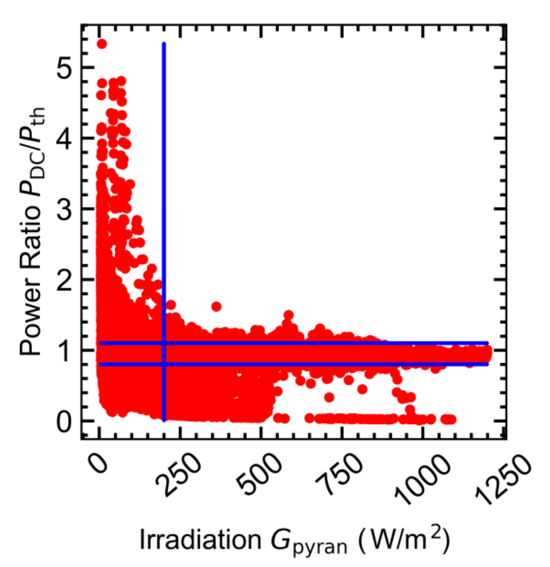
To further examine the acquired data quality, feature correlations were performed. In particular, the correlations used were based on the power ratio of the measured DC power ($P_{\mathrm{out},\mathrm{t}}$) and the maximum temperature corrected theoretical power ($P_{\mathrm{th},\mathrm{t}}$), given by:

$$P_{\mathrm{th},\mathrm{t}}=G_{\mathrm{i}} A_{\mathrm{a}} {\eta }_{\mathrm{A},0} C_{\mathrm{t}}$$

(1)

where $G_{\mathrm{i}}$ is the in-plane irradiance, $A_{\mathrm{a}}$ is the overall array area, ${\eta }_{\mathrm{A},0}$ is the rated array efficiency and $C_{\mathrm{t}}$ is the power rating temperature adjustment factor as follows [32]:

$$C_{\mathrm{t}}=1+\gamma \left({{\rm T}}_{\mathrm{mod},\mathrm{k}}-25 °\mathrm{C}\right)$$

(2)

where $\gamma$ is the relative maximum power temperature coefficient (in units of °C⁻¹) and ${{\rm T}}_{\mathrm{mod},\mathrm{k}}$ is the module temperature (in °C) in time interval $k$.

Furthermore, the rated array efficiency, ${\eta }_{\mathrm{A},0}$ is calculated by [32]:

$${\eta }_{\mathrm{A},0}=P_{\mathrm{o}}/\left(G_{\mathrm{i},\mathrm{ref}} A_{\mathrm{a}}\right)$$

(3)

where $P_{\mathrm{o}}$ is the nominal power and $G_{\mathrm{i},\mathrm{ref}}$ is the reference global solar irradiance of 1000 W/m².

An exemplary correlation between the power ratio and the solar irradiance is shown in Figure 2. It is obvious from the plot that a lot of datasets are not aligned to the theoretical possible optimum. For an accurate analysis of the $R_D$, all erroneous dataset points, which may have occurred due to shading, snow and overall outliers, can be filtered by only considering data points around the theoretical optimum and set threshold levels. In particular, to account for measurement uncertainties, the threshold acceptable window was set lower than $P_{\mathrm{th},\mathrm{t}}\times 1.1$ and higher than $P_{\mathrm{th},\mathrm{t}}\times 0.8$.

Additionally, a second irradiance filter was introduced after the initial data quality filtering step, in order to filter out data occurring lower than $G_{\mathrm{i}}=200 \mathrm{W}/{\mathrm{m}}^2$. This criterion was set to reduce the size of the data while at the same time ensure that no useful performance information is lost.

2.3. Performance Ratio

The performance metric adopted in this study was the performance ratio, $PR$, because of its increasing use to characterize system performance and due to the removal of the most important first-order driver of system output, namely, the incident POA irradiance. This performance metric is largely independent of the incident solar irradiance on the PV system and for this reason it is widely used to compare the performance of PV systems at different locations, focusing only on the overall loss factors. In this context, the PR metric was used in order to fully capture all environmental loss factors and PV system efficiency losses over a predefined recording period. The IEC-61724:2017 [32], defines different ways to calculate the $PR$. In this work, the $PR$ is calculated as follows [32]:

$$PR=({\displaystyle \sum }_k\frac{P_{\mathrm{out},\mathrm{t}}\times {\tau }_k}{P_0})/({\displaystyle \sum }_k\frac{G_{\mathrm{i},\mathrm{k}}\times {\tau }_k}{G_{\mathrm{i},\mathrm{ref}}})$$

(4)

where $P_{\mathrm{out},\mathrm{k}}$ is the measured DC power output per time step, ${\tau }_k$ is the time step, $P_{\mathrm{o}}$ is the nominal power, $G_{\mathrm{i},\mathrm{k}}$ is the in-plane solar irradiance per time step and $G_{\mathrm{i},\mathrm{ref}}$ is the reference solar irradiance of 1000 W/m².

Even though the $PR$ can be calculated at different time resolutions (daily, weekly or monthly), for this investigation the monthly resolution was selected since it provides the necessary accuracy without adding too much noise compared to a daily resolution. For each PV system the 1-minute resolution datasets extracted from the data quality and filtering step were used to construct monthly $PR$ time series over the 12-year evaluation period.

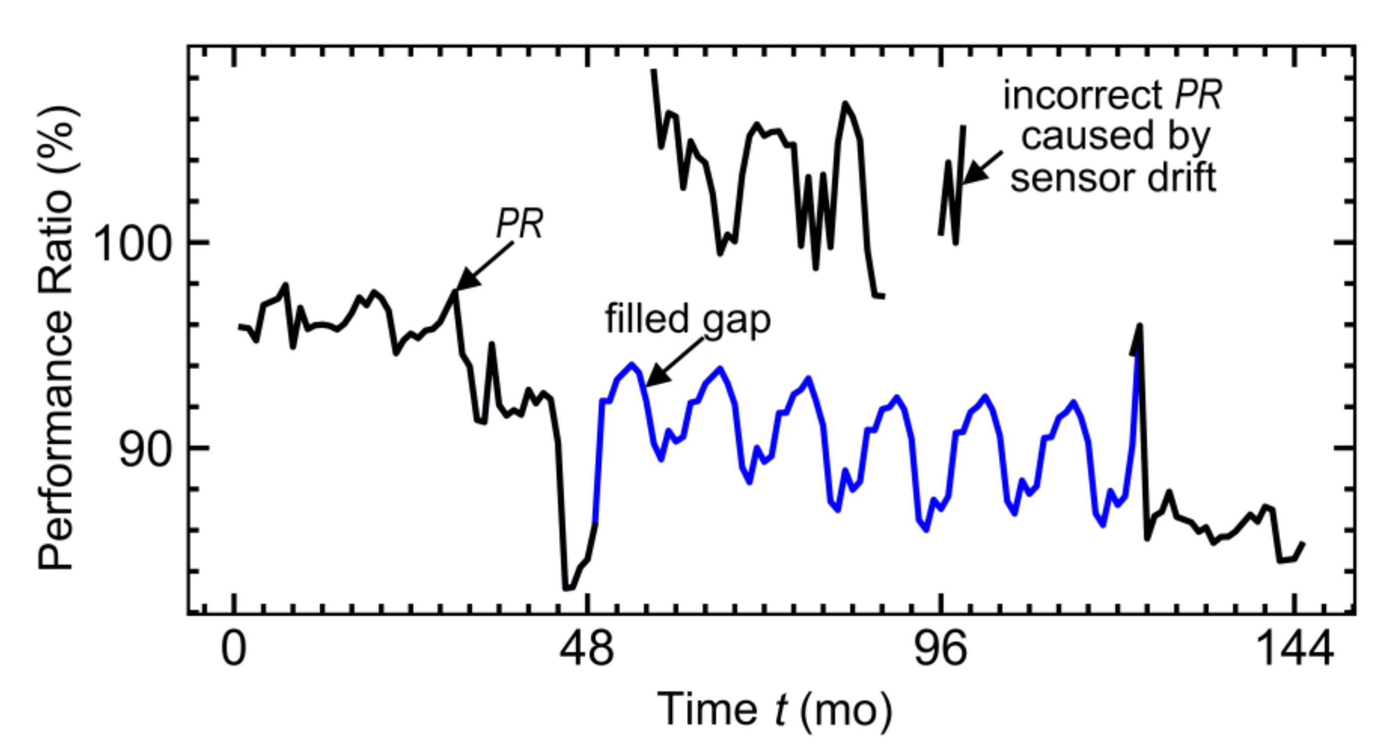
2.4. Time Series Reconstruction and Imputation

A data detection routine was subsequently applied to the constructed monthly $PR$ time series of each PV system, in order to identify missing values and gap periods attributed to sensor and DAQ system failures. 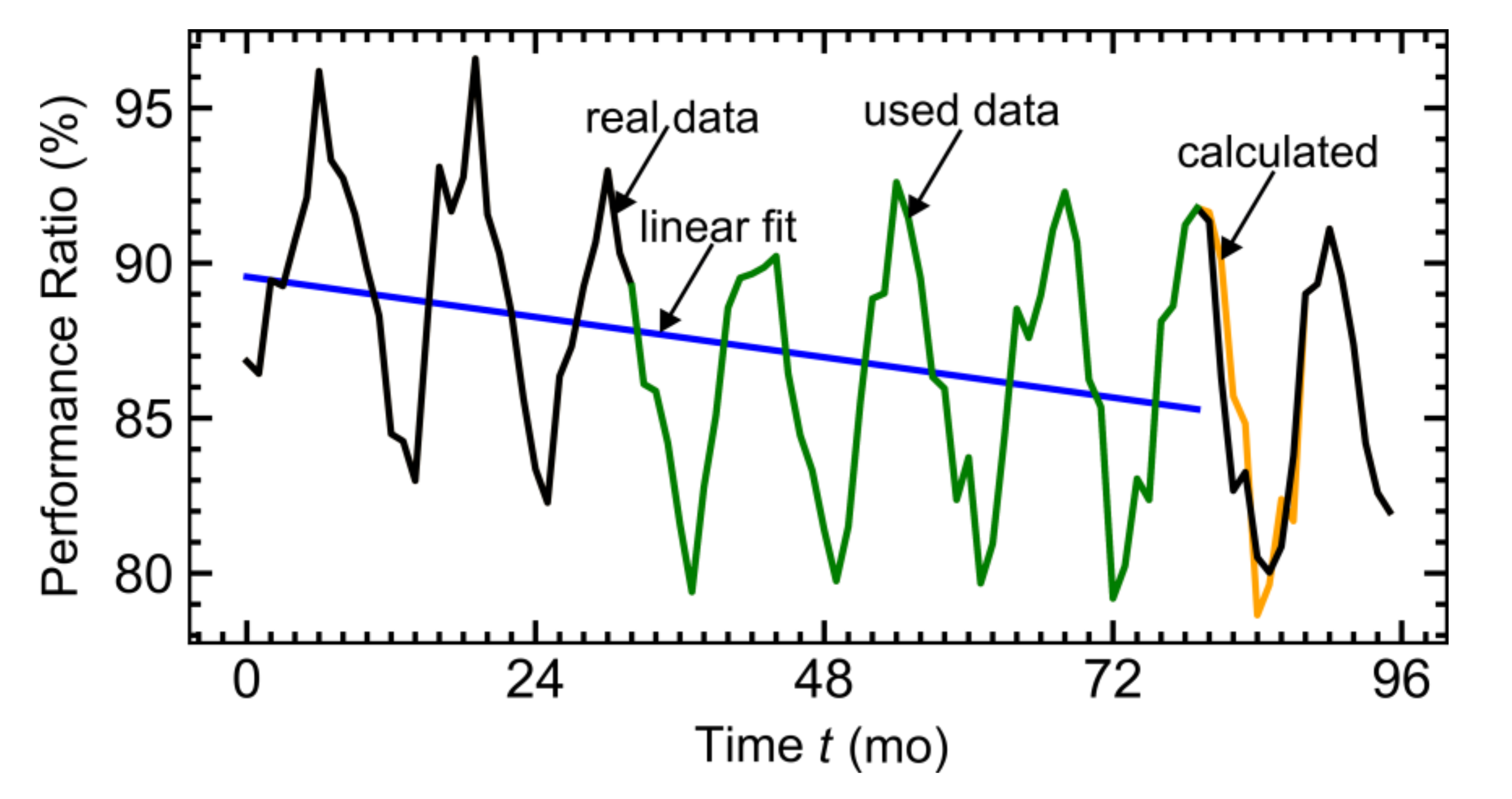The detected missing values and gaps were treated by either applying linear interpolation in the case that the monthly $PR$ gap occurred during the first year whereas in the case that the monthly $PR$ gap occurred after the first year, the missing value was calculated based on a naïve method that considered the value as being the same as the respective monthly $PR$ value of the previous year. Furthermore, if a gap was detected in the subsequent years, then the historic monthly mean of the previous respective months of the 3 preceding years was used to fill the missing gap. A typical example time series reconstruction and imputation algorithm application to reconstruct missing monthly $PR$ values is depicted in Figure 3. The green plot shows the values used (preceding 3-year monthly $PR$ values were used) to calculate the reconstructed datapoints. The orange plot shows the reconstructed monthly $PR$ values that were in close agreement to the actual data.

2.5. Time Series Analytical Techniques

In the previous steps, the monthly $PR$ time series of each PV system were constructed and data quality validated, in order to be used for the $R_D$ analysis. In this part of the process, the yearly $R_D$ of each investigated PV system were calculated by employing data-driven statistical time series techniques, namely the OLS, CSD, STL, ARIMA, RCPA and YOY.

2.5.1. Ordinary Least Squares

The most widely adopted time series analytical typical technique to calculate the $R_D$ is OLS. The linear regression uses the least-squares method, which minimizes the distance between each datapoint and an assumed straight line (residual). This technique was applied to the monthly $PR$ time series of each system according to:

$$Y=a X+b$$

(5)

where $a$ is the slope of the linear fit and $b$ is the y axis intercept.

The absolute yearly $R_D$ was calculated for each PV system using the gradient of the obtained linear fit and multiplying it by the number of months in a year [16].

2.5.2. Classical Series Decomposition

Time series data can be split into the trend, which shows the basic direction of the analyzed data from which basically the $R_D$ can be derived from, the seasonality factor (in PV, this can be induced due to external factors such as weather and can be observed in fluctuations of the $PR$ in winter and summer) and the noise or irregular part.

CSD is a time series decomposition technique that is commonly used to extract the underlying trend from the series with the application of a centered moving average [33,34]. A two-step centered moving average is used in order to obtain the trend from the time series. Furthermore, for a $2 x k$ moving average, the centred moving average at time $t$ used to find the trend at time $t$, $T_{\mathrm{t}}$, is as follows:

$$T_{\mathrm{t}}=\frac{1}{2}\left(\frac{1}{k}{\displaystyle \sum }_{i=t-m}^{t+m-1}{Y}_{\mathrm{i}}+\frac{1}{k}{\displaystyle \sum }_{i=t-m+1}^{t+m}{Y}_{\mathrm{i}}\right)$$

(6)

where $k$ is the moving average order and $m$ is equal to the half-width of a moving average.

In this study, this technique was applied to the monthly $PR$ time series of the PV systems in order to extract the trend, the seasonality and the irregular component. The order of the moving average for each investigated PV system was equal to 12 because of the number of months per year.

Finally, linear regression was applied to the extracted trend in order to calculate the yearly $R_D$.

2.5.3. Seasonal and Trend Decomposition Using Loess

Similarly to CSD, the STL method decomposes a seasonal time-series into the following components: seasonal, trend and remainder [33], by performing an inner and an outer loop. The trend and the seasonal components are updated when a run in the inner loop takes place, which are equal to 1 or 2. The outer loop has an inner loop and it is followed by an estimation of accurate weights that works as an input for the next inner loop in order to decrease the impact of transient, abnormal behavior on the trend and seasonal parts [34].

2.5.4. Autoregressive Integrated Moving Average

The ARIMA method is a generalization of the autoregressive moving average (ARMA) model and consists of two parts, the autoregressive (AR) and the weighted moving average (MA). Both models can be used to better understand the time series data and forecast future developments of data. The integrated part (I), which differs the ARMA model from the ARIMA model, means that an initial differentiating step can be applied one or more times to remove the present non-stationary. The non-stationary share describes the searched $R_D$ as a trend.

ARIMA models essentially consist of 3 main parts. In the first part, certain properties of the time series are characterized using autoregressive approaches. Subsequently, these properties are used in the second part to estimate the seasonality. In the end, the third part is the diagnostic testing performed in order to validate the results.

For this investigation, after the ARIMA model was constructed and the trend was successfully calculated, alike the degradation calculation of CSD and STL, a linear regression was applied and the yearly $R_D$ was calculated for each PV system by using the gradient obtained from each fit.

2.5.5. Robust Principal Component Analysis

RPCA is a method that reduces the dimensionality of multivariate data by creating an optimal superposition of the original variables with respect to the Euclidean norm. This is a linear algebraic tool that describes the geometrical characteristics of multivariate statistical data. The original data matrix is called $A$ and it can be expressed as follows:

$$A=D+P$$

(7)

where $D$ is a low rank data matrix that indicates the number of characteristic features dominating the $A$ matrix and $P$ is the perturbation matrix that causes the outliers [14].

RPCA reduces the dimensions of the time-series into the PCs, which were then used to calculate the performance metrics of the first and last year of the evaluation period. The low-rank matrix ($D$) could then be used for further calculations of the $R_D$ and the perturbation matrix ($P$) could be disregarded.

In the scope of calculating the yearly $R_D$ of PV systems, the low-rank matrix contains the $PR$ of each year in each column of the matrix. The yearly $R_D$ was calculated by comparing the change of the integral of the first and last year monthly $PR$. More specifically, the integrals describe the area of the respective year one $A_1$ and the last year $A_n$. The change of both areas was then divided by the reference area of the first year $A_1$ and the number of considered years $n$, to yield the $R_D$:

$$R_D=\frac{A_1-A_n}{A_1 n}$$

(8)

2.5.6. Year-on-Year

The YoY technique was proposed by the National Renewable Energy Laboratory (NREL) of the U.S. Department of Energy [7] as a comparative data point method between subsequent years, where the $R_D$ was calculated as a comparison of the data points of the same month, week or day. This procedure was then repeated for every data point of subsequent years.

After each individual $R_D$ was calculated, the YoY technique appended these values in a list of successive data points from one date to the same date in the following year. The list obtained by this procedure was then sorted in either an ascending or descending order.

Finally, the sorted list was used to obtain the median value, which represents the $R_D$ of the investigated PV system. By using the median value over the mean, the YoY was more robust (less prone) to outliers in comparison to the mean value. The median value was used as the yearly $R_D$ for the investigated PV systems in this analysis.

2.6. Long-Term Degradation Components

In general, the long-term $R_D$ calculated using techniques applied to constructed performance time series depends on the quality of the components that affect degradation (degradation of PV modules and inverter), maintenance intensity from one year to another (soiling, snow, shading and failure repair duration), variation of climate condition change from one year to another (solar irradiation and ambient temperature) and component failures (PV module hot-spots, cracks, corrosion, delamination, glass breakage, cell interconnection breakage, diode failures and balance of system and inverter component failures). In this study, all necessary measures were taken in order to specifically exclude the influence of maintenance intensity and yearly irradiation variation. In more detail, the $R_D$ part due to the maintenance intensity was minimized since an initial step before calculating the long-term $R_D$ was to discard all data that were affected from soiling, shading and failure repairs (initially applied data quality filtering stage). According to a recent survey, the overall yearly soiling loss for modules installed at a tilt angle >15° for the Köppen–Geiger classification of the PV systems installed in Nicosia, Cyprus and Stuttgart, Germany is 4% and 0.5%, respectively [35]. Assuming therefore that the arrays were only cleaned once a year and by rain, this would have reflected to a maximum soiling contribution of 0.33%/year and 0.04%/year to the long-term $R_D$ for the systems in Cyprus and Stuttgart, respectively. However, this effect of dust and also snow was mitigated since the arrays were periodically cleaned (seasonal cleaning and after dust events or snow accumulation every year for this investigation).

The impact of climate variations to the long-term $R_D$ was investigated by analyzing the exhibited variation of both the in-plane global irradiation and module temperature of each system over the 12-year evaluation period. Specifically, the analysis included the calculation of the yearly variation of the measured in-plane global irradiation and module temperature at both locations and translating the obtained values to performance loss rate components that could be mapped to the $R_D$.

Finally, the impact of component failures to the $R_D$, was further analyzed since two PV systems (sw165Ni multi-c-Si and bp185Ni mono-c-Si) exhibited failures that were detected through the regular on-site O&M inspections (visual inspections, thermal imaging and I–V tracing). In particular, a hot-spot at a module of the sw165Ni multi-c-Si and the bp185Ni mono-c-Si PV systems was detected in the 4th (September 2010, month 52) and 7th year of operation (June 2013, month 85), respectively. According to a review study on the failures of PV modules performed by the International Energy Agency (IEA) photovoltaic power systems (PVPS) Taskforce 13, the power loss category for a hot-spot failure is A, which denotes power loss below the detection limit of <3% [36]. The impact assessment of this failure on the long-term $R_D$ for these systems was calculated using the approach presented in [37]. First, the $R_D$ of a specific module with failure $x$ ($d_{i,x}$) was calculated by [37]:

$$d_{i,x}=\frac{\Delta P_{i,x}}{{\tau }_{b,i}-{\tau }_{a,i}}$$

(9)

where $\Delta P_{i,x}$ is the power loss of the specific module given in percentage, ${\tau }_{b,x}$ is the date of failure documentation of dataset $i$ and ${\tau }_{a,x}$ is the date of system start of dataset $i$.

The equation for the $R_D$ failure impact of the whole system (${\delta }_{i,x}$) is given by [37]:

$${\delta }_{i,x}=d_{i,x}\frac{z_i}{y_i}$$

(10)

where $z_i$ is the percentage of the system being affected by the failure and $y_i$ is the investigated system part in percent from the total nominal system power $P_i$.

3. Results

3.1. Data Quality Filtering and Time Series Reconstruction

The $R_D$ location-dependency comparison of both locations is of interest due to their differences in the climatic conditions. The yearly global solar irradiation in Nicosia, Cyprus (2000 kWh/m²) was approximately 70% higher compared to Stuttgart, Germany (1100 kWh/m²). Furthermore, the higher irradiation was clearly reflected to the amount of sun hours per year, with 3310 h in Nicosia compared to 1800 h in Stuttgart. 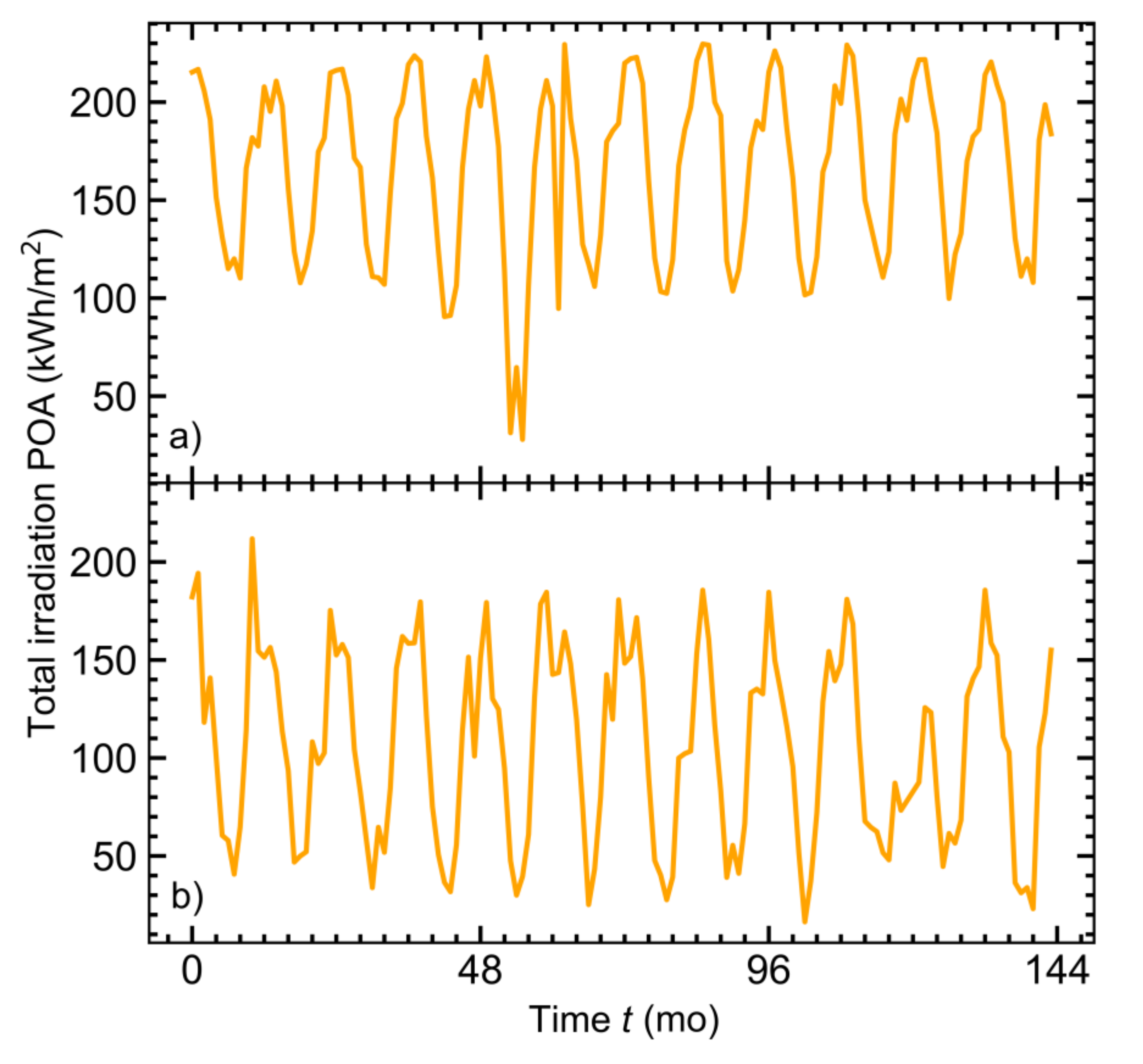The mean yearly ambient temperature in Nicosia, Cyprus was 19.7 °C, which is 110% higher compared to Stuttgart, Germany at 9.4 °C [38,39]. The exhibited monthly total irradiation at the POA at both locations over the 12-year evaluation period is provided in Figure 4. The irradiation plots at both locations exhibited a monotonic trend behavior.

The initial application of the proposed data quality and filtering step to the acquired 1-minute datasets indicated that some of the installed sensors exhibited abnormal behavior (sensor drifts prior to a complete sensor failure, which resulted in erroneous data and outage periods) after several years of outdoor operation, at both location sites.

Figure 5 shows a typical example (ase170St multi-c-Si PV system installed in Stuttgart, Germany) of the acquired 1-minute datasets monthly data availability, after the application of the initial data quality and irradiance filtering steps. Based on the on-site outage log records, the specific system had a measurement sensor failure throughout the third, fourth and fifth operational years. The plots clearly demonstrated that data was available for this system apart from the period between months 32 and 60 (no data availability is represented as zero). Additionally, the application of both filtering steps reduced the percentile availability of the winter season datasets by a higher magnitude compared to the summer due to the high amount of low-irradiance datapoints present during the winter and prolonged night-time. Specifically, the application of the second step irradiance filter further reduced the data by approximately 20%. The fact that a large share of data was filtered out from the initial 12-year dataset provided evidence that the data quality and filtering step is necessary in order to ensure data fidelity for the subsequent analysis.

As observed in Figure 6, the missing dataset gaps were successfully imputed and the monthly $PR$ time series was reconstructed for months 32–60, using the time series reconstruction algorithm. In particular, the data gaps due to the measurement equipment failure were reconstructed with accurate estimates, since the estimated monthly $PR$ values were comparable to exhibited values of the prior and posterior years. The imputation results further indicated that 3 consecutive prior years of data were adequate to fill the gap and estimate the $PR$ for the ase170St multi-c-Si PV system in Stuttgart, Germany.

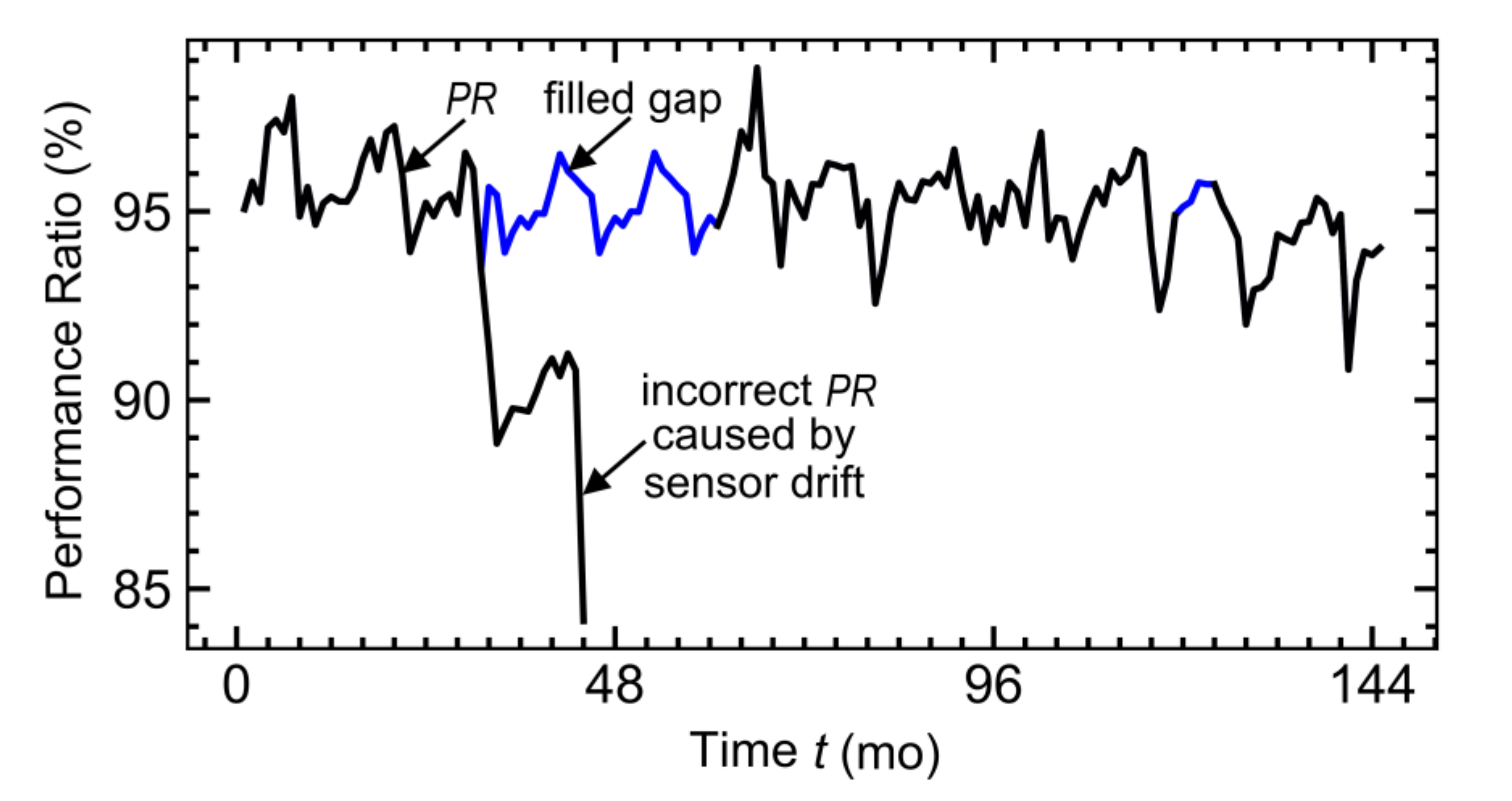
The robustness of the time series reconstruction and imputation algorithm was further verified by applying the algorithm to reconstruct the time monthly $PR$ series of the multi-c-Si sw165St PV system in Stuttgart, Germany. Figure 7 shows that the reconstruction algorithm was able to impute the time series missing gaps and sensor drifts identified for months 50–120, by utilizing the prior 3-year values.

Even though in some cases the datasets exhibited huge gaps, the filling gaps algorithm was able to reconstruct the missing values in a very reliable manner. This was proven by comparing the predicted filled gaps performance ratio and the performance ratio, which could be calculated after the sensor change. This led to the finding that the filling gaps algorithm worked properly, even for gaps of up to 4 years. Specifically, filling data gaps of up to 4 years proved to be possible in case the monthly $PR$ datapoints of the starting years was of high quality and could be proven with ending years of high quality. Longer data gaps led to an overestimation of the performance ratio. Hence, ensuring high measurement quality in the first 3–5 years is of great importance to calculate the degradation of the PV power system.

3.2. Degradation Rates of PV Systems

The techniques of OLS, CSD, STL, ARIMA, RPCA and YoY were applied to the constructed and data quality verified monthly $PR$ time series of the investigated PV systems at both locations, in order to calculate the yearly $R_D$. The seasonal effects were considered by setting the $R_D$ to begin from year 3 and extend towards the last year of the investigation. Additionally, the accuracy of each time series analytical technique to calculate the yearly $R_D$ was benchmarked against the obtained $R_D$ obtained during the 8th year using indoor standardized test procedures and a solar simulator to determine the maximum power of each system as per IEC 61215 [29]. The obtained $R_D$ was assumed to exhibit a linear behaviour and constant over time. 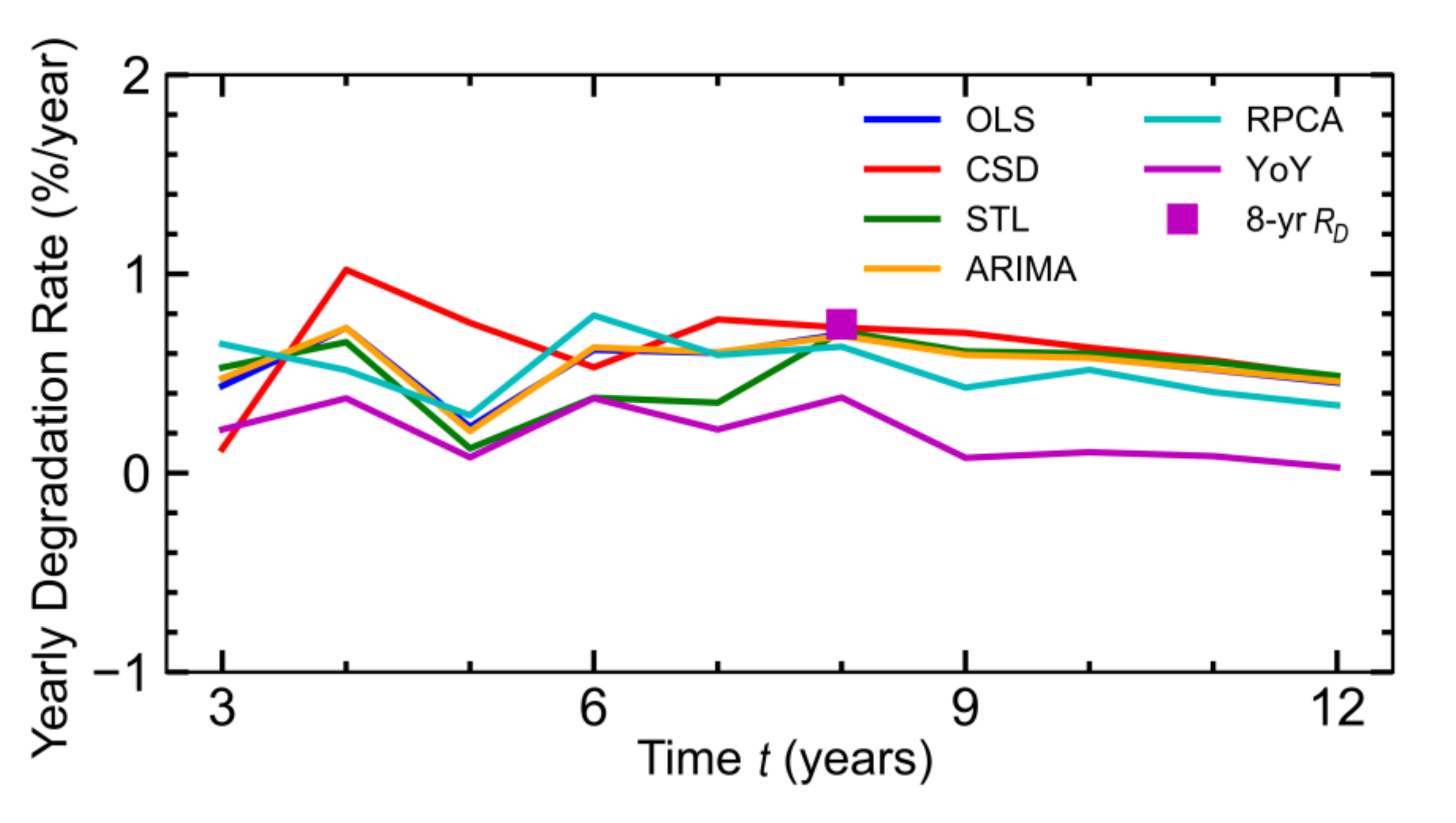Figure 8 shows the course of the yearly $R_D$ of the multi-c-Si system ase170Ni in Nicosia, Cyprus calculated with all the time series analytical techniques over the 12-year period. The results demonstrated that all the applied techniques exhibit similar performance since the maximum absolute difference between the obtained results for each investigated duration was <1%/year. Almost all techniques appeared to converge after 7 years of analysis, since the maximum absolute difference between the $R_D$ values was 0.2%/year. Another important outcome was obtained from the comparative 8-year $R_D$ analysis obtained indoors at STC and the time series techniques. The obtained results exhibited close agreement and overlap, providing scientific evidence that the adoption of time series technique is only crucial if the quality of data is low, otherwise simple methods such as the OLS yield accurate results and are applicable for $R_D$ studies. The fact that less sophisticated $R_D$ techniques (OLS, CSD and STL) exhibited close agreement to the indoor standardized test procedure results renders these techniques applicable for $R_D$ studies and favourable over other elaborate and computer intensive techniques.

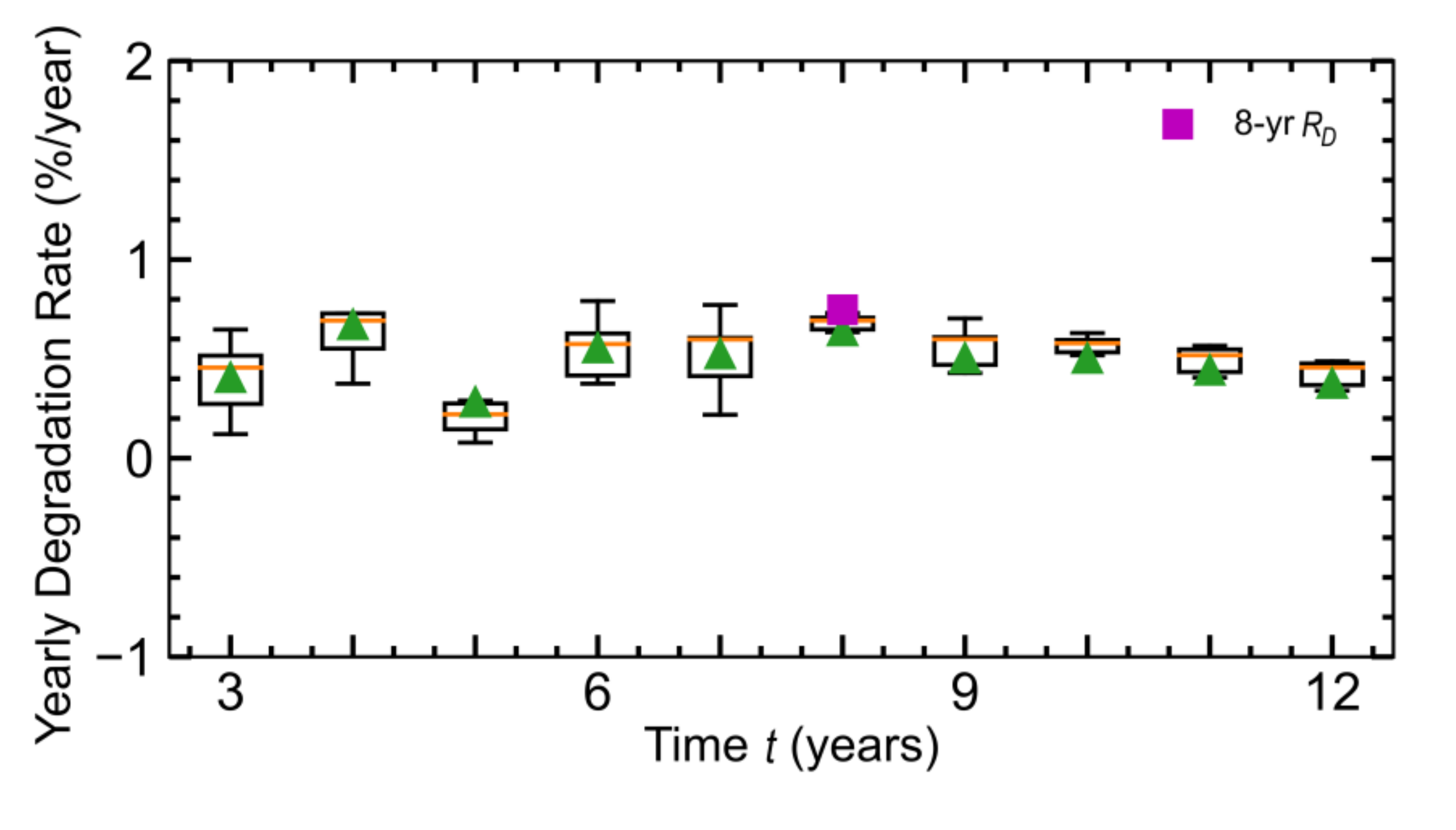
Furthermore, Figure 9 shows the box-plot of the calculated yearly $R_D$ over the 12-year evaluation period for the ase170Ni multi-c-Si PV system. The median value is displayed with an orange horizontal bar while the mean is depicted as a green triangle. The results indicated that for the high quality, filtered and reconstructed time series of this investigation, the adoption of which time series analytical technique is irrelevant and the results will be similar, since the standard deviation of the results (width of each box) is narrow.

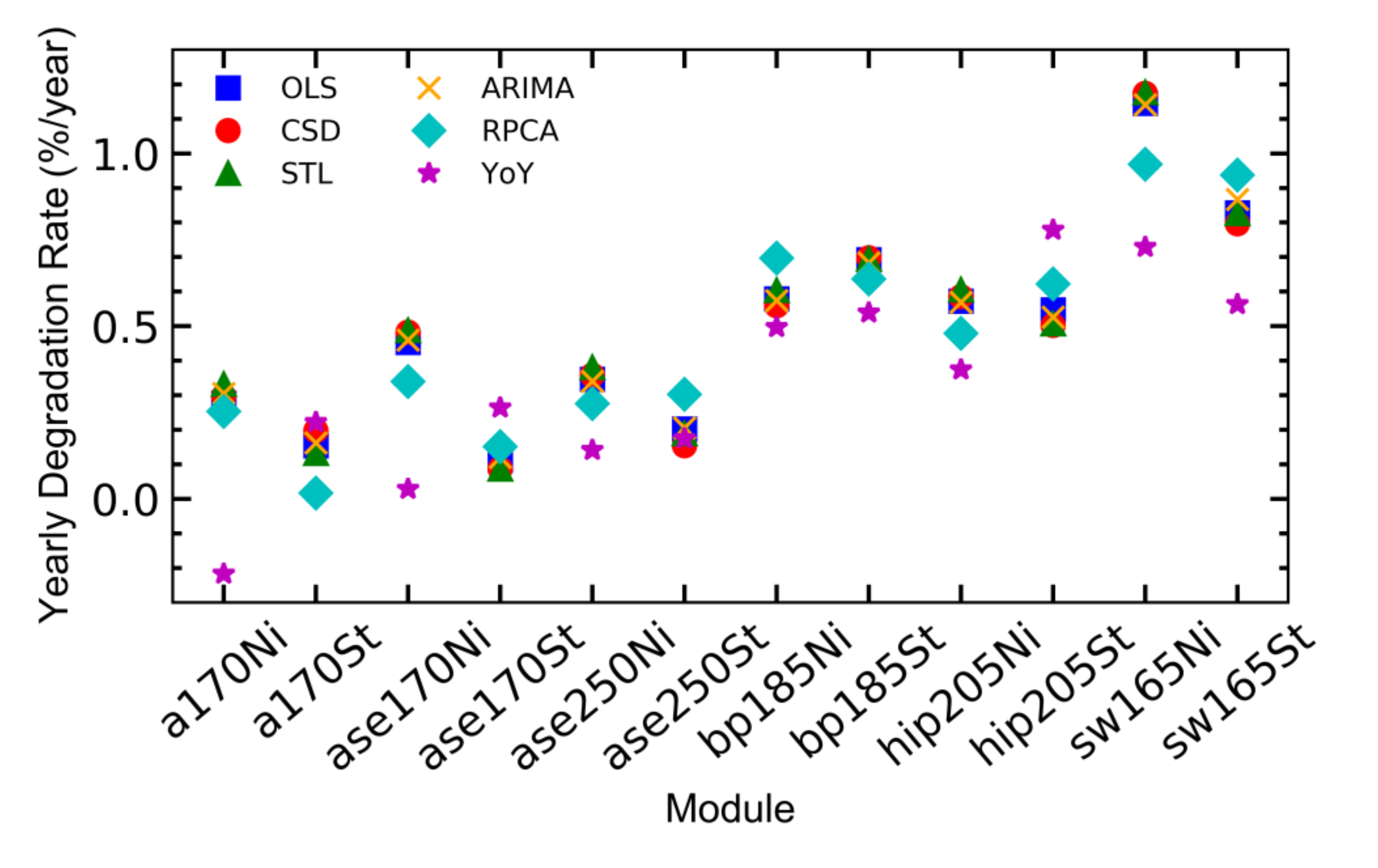
The long-term yearly $R_D$ of all the investigated c-Si PV systems at both locations over the 12-year evaluation period are presented in Figure 10. Overall, the results demonstrated that the a170 mono-c-Si system and all multi-c-Si systems (ase170, ase250 and sw165) presented higher $R_D$ in Nicosia, Cyprus (>0.1%/year absolute difference) compared to the results obtained in Stuttgart, Germany for all the applied time series de-trending techniques (OLS, CSD, ARIMA and STL). The only technique that showed a higher $R_D$ in Stuttgart, Germany for systems a170 mono-c-Si and ase170 multi-c-Si was YoY. The YoY technique yielded the lowest $R_D$ values for almost all of the PV systems. In general, the YoY technique is more prone to erroneous data due to the fact that erroneous monthly $PR$ shifts the median. The reason why PV systems such as the sw165Ni multi-c-Si PV system showed wider variations in the exhibited results specifically the YoY technique is attributed to failures such as hot spots that deteriorated in a non-linear manner the performance of the system. Accordingly, the application of RPCA resulted in most cases to higher $R_D$ values compared to the other applied time series analytical techniques. The RPCA technique is also prone to erroneous data of the first and last year as result of only using the data of those years. Hence, if the data of the last year is affected by a sensor drift or erroneous data, then the $R_D$ will differ from the $R_D$ of other methods that also take all the other years into account.

Additionally, the only system with higher $R_D$ in Stuttgart, Germany compared to Nicosia, Cyprus is the bp185 mono-c-Si (0.1%/year absolute difference) for all the time series detrending techniques. The hip205 mono-c-Si system yielded similar results for both locations (<0.1%/year absolute difference).

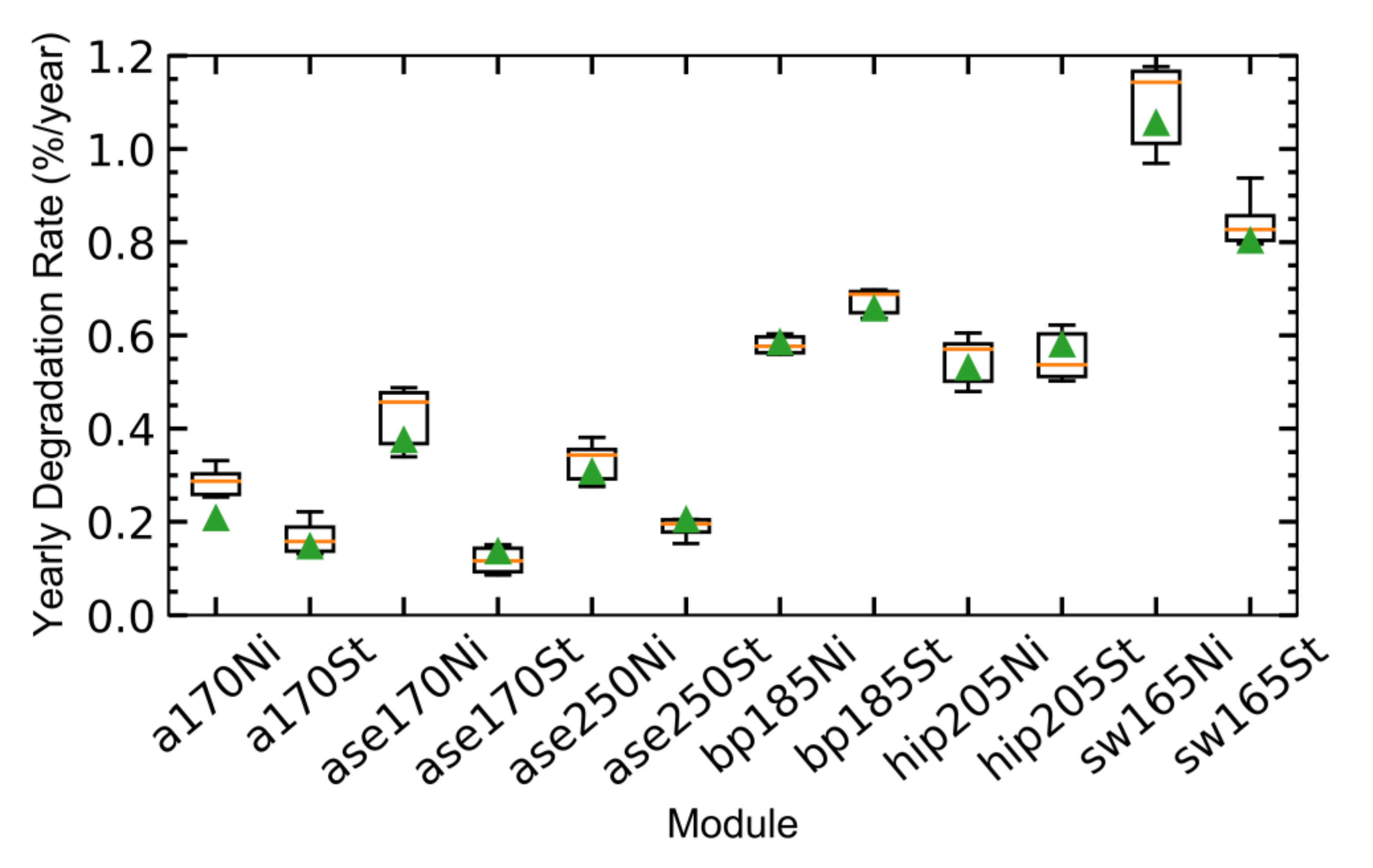
3.3. Long-Term Degradation Location Dependency

To evaluate the location-dependency of the exhibited degradation, a box-plot of the yearly $R_D$ over the 12-year evaluation period for each PV system at both locations was constructed and depicted in Figure 11. The box-plot demonstrates that the median $R_D$ value, displayed in orange color, of most of the investigated PV systems was slightly higher in Nicosia, Cyprus compared to Stuttgart, Germany. Along this context, an important outcome from this plot was that the calculated degradation for most of the PV systems installed at the warm climate of Nicosia, Cyprus was higher compared to the respective systems at the moderate climate of Stuttgart, Germany. More specifically, by comparing the median value of the obtained results from the applied techniques, all the multi-c-Si technologies (ase170, ase250 and sw165) exhibited higher $R_D$ (>0.1%/year absolute difference) in Nicosia, Cyprus compared to Stuttgart, Germany. This demonstrated that the $R_D$ of the investigated multi-c-Si technologies was affected by the installation location. For the mono-c-Si technologies, the a170 system showed a higher degradation in Nicosia, Cyprus compared to Stuttgart, Germany (>0.1%/year absolute difference), while the bp185 mono-c-Si system showed a higher degradation in Stuttgart, Germany (>0.1%/year absolute difference). The hip205 mono-c-Si system exhibited similar results since the absolute difference of median values of both locations were <0.1%/year.

In summary, the obtained results showed that the $R_D$ of the investigated multi-c-Si systems was location dependent since higher absolute differences in the range of 0.1–0.4%/year, were obtained compared to the respective systems in Stuttgart, Germany. For the mono-c-Si systems the results demonstrated that the $R_D$ location-dependency was also affected by the manufacturing technology.

For all the investigated PV systems in this study, apart from the sw165Ni multi-c-Si and the bp185Ni mono-c-Si PV systems, which exhibited failures, the calculated long-term $R_D$ was mainly attributed to the degradation of the system components (ageing due to material deterioration over time, light induced degradation (LID), potential induced degradation (PID) and weathering due to environmental effects). With respect to the impact of the yearly irradiation variation to the long-term $R_D$, the analysis showed that in Nicosia, Cyprus and Stuttgart, Germany the yearly in-plane global irradiation variation was 99 kWh/m²/year (5% when normalized to the average yearly irradiation of the 12-year period, 1994 kWh/m²) and 95 kWh/m²/year (7% when normalized to the average yearly irradiation of the 12-year period, 1267 kWh/m²), respectively. However, in this investigation the $R_D$ was calculated using the $PR$ as the time series metric and this provides the advantage that the performance values were normalized to the irradiance, hence not affected by any variation in the monthly or yearly irradiation. Similarly, the variation of the yearly average module temperature on the $R_D$ of each PV system demonstrated that in Nicosia, Cyprus and Stuttgart, Germany the highest yearly module temperature variation was 0.55 °C and 0.84 °C, respectively. These values were then multiplied by the power temperature coefficient of each technology and subsequently divided by the evaluation period (12 years) in order to yield a maximum performance loss rate thermal variation component affecting the $R_D$, of 0.02%/year and 0.03%/year for the systems in Cyprus and Germany, respectively.

Furthermore, the $R_D$ part due to maintenance intensity from one year to another was minimized in this investigation since before calculating the long-term $R_D$, an initial step taken was to discard through the filtering data quality stage the effect of soiling, shading and failure repairs. Additionally, the PV arrays were periodically cleaned (seasonal cleaning) and after dust events or snow accumulation in order to minimize these effects.

Finally, regarding, the hot-spot failures detected for the sw165Ni multi-c-Si and the bp185Ni mono-c-Si PV systems, the analysis showed that the impact of these failures on the long-term $R_D$ is 0.13%/year and 0.08%/year, respectively.

4. Discussion

In this work, a comparative analysis of the yearly $R_D$ exhibited by identical c-Si PV systems installed at different locations (Nicosia, Cyprus Köppen–Geiger: Mid-Latitude Steppe and Desert Climate and Stuttgart, Germany Köppen–Geiger: Marine West Coast Climate) was performed, in order to present a unified robust methodology for accurately calculating the $R_D$ of PV systems from outdoor monitored measurements and assess the location dependency of degradation mechanisms. In summary, the following findings were obtained throughout the commenced analysis:

• The application of the proposed data quality and filtering steps ensured data fidelity for the subsequent analysis while at the same time reducing the size of the datasets. The fact that a large share of data was filtered out and yet the calculated $R_D$ values were comparable to the indoor applied standardized procedures renders the data inference stage necessary for performance assessments.
• The data imputation and time series reconstruction algorithm proved reliable in filling missing data and gaps. The algorithm was able to reconstruct the performance metric time series with accurate estimates, since the estimated monthly values were comparable to exhibited values of the previous years. The imputation results further indicated that 3 consecutive years of data were adequate to fill the gap and estimate the missing points.
• Irrespective of the applied time series analytical technique to calculate the yearly $R_D$ of PV systems, the results showed minor differences for almost all techniques, after converging in a time frame of 7 years.
• Overall, the adoption of the time series technique did not show significant differences in the resulting $R_D$ values. This renders less sophisticated $R_D$ techniques (OLS, CSD and STL) applicable for $R_D$ studies and favorable over other elaborate and computer intensive techniques.
• The long-term $R_D$ results demonstrated that most of the systems installed at the warm climatic conditions in Nicosia, Cyprus were degrading at a higher rate compared to their counterparts at the moderate climate of Stuttgart, Germany. More specifically, all multi-c-Si technologies showed higher degradation results in Nicosia, Cyprus for all applied de-trending time series techniques. Several reasons to explain this effect include the exposure of the lamination foil to higher irradiation, which leads to higher rates of discoloration over time and a decrease of the transparency. The warm temperature may influence the changes in the crystalline structure of the cells or interconnection stresses due to the high thermal cycles. Other factors can be scratches on the glass surface of the panels as a result of the higher dust content in the air coming from the Sahara Desert and which also leads to a decrease of the transparency. On the other hand, only the a170 mono-c-Si system exhibited higher $R_D$ values in Nicosia, Cyprus. The remaining mono-c-Si technologies bp185 and hip205 showed lower and similar degradations when compared to the results obtained for all applied detrending time series techniques to the systems in Stuttgart, Germany, respectively.
• This study verified that the degradation assumed by the manufacturers of the modules, was underscored and a life time extension might be possible.

Finally, as the leading question of this study was to investigate whether the degradation of PV systems is location dependent, the obtained long-term yearly $R_D$ results indicated that the degradation of the investigated multi-c-Si systems is location dependent since higher absolute differences, in the range of 0.1-–0.4%/year, were obtained compared to the respective systems in Stuttgart, Germany. For the mono-c-Si systems the results demonstrated that the $R_D$ location-dependency is also affected by the manufacturing technology. Even though the results provide evidence that warmer climates influence the degradation of the systems, it must be noted that the results are limited to the specific technologies and production batch and for this reason these findings might not entirely apply to newer manufacturing line technologies. Hence, further research studies are needed to investigate whether the observed behavior can be generalized to latest technology PV modules at other climatic conditions and for other latest technologies.

5. Conclusions

This paper presents the analysis performed to implement a unified methodology for accurately calculating the $R_D$ of grid-connected PV systems and provides evidence of the $R_D$ location-dependency. The method included the application of data inference and time series analytics to high-resolution 1-minute datasets acquired from different c-Si PV systems, installed and monitored at two different climatic locations (warm climate of Nicosia, Cyprus and moderate climate in Stuttgart, Germany).

The obtained $R_D$ results demonstrated that the application of the data quality and filtering steps ensured data fidelity and proved to be necessary since the results obtained from the inferred data were comparable to indoor applied standardized procedures.

Additionally, the adoption of time series technique proved insignificant once the underlying dataset was of high fidelity. More specifically, the yearly $R_D$ results showed minor differences for almost all techniques, after converging in a time frame of 7 years. This established less sophisticated $R_D$ techniques (OLS, CSD and STL) applicable for $R_D$ studies.

Furthermore, the long-term $R_D$ comparative analysis showed that the multi-c-Si PV systems installed at the warm climatic conditions in Nicosia, Cyprus were degrading at a higher rate compared to their counterparts at the moderate climate of Stuttgart, Germany (absolute difference in the yearly $R_D$ in the range of 0.1%/year to 0.4%/year). This provided adequate evidence and verified the initial hypothesis that degradation mechanisms are location dependent for the investigated multi-c-Si technologies. For the mono-c-Si systems the results demonstrated that the $R_D$ location-dependency was also affected by the manufacturing technology.

Finally, the manufacturers of the PV modules planned a degradation of around 1.0%/year. This value was almost always undershot by all modules, which showed a lower degradation during the considered time period. Hence, a lifetime extension of these modules can be taken into consideration and might also be applicable for current technologies.