
A Practical Load Disaggregation Approach for Monitoring Industrial Users Demand with Limited Data Availability


Abstract
:1. Introduction
1.1. Industrial DSM and the Need for Load Disaggregation
1.2. Load Disaggregation Approaches
1.3. Industrial DSM Projects across the World
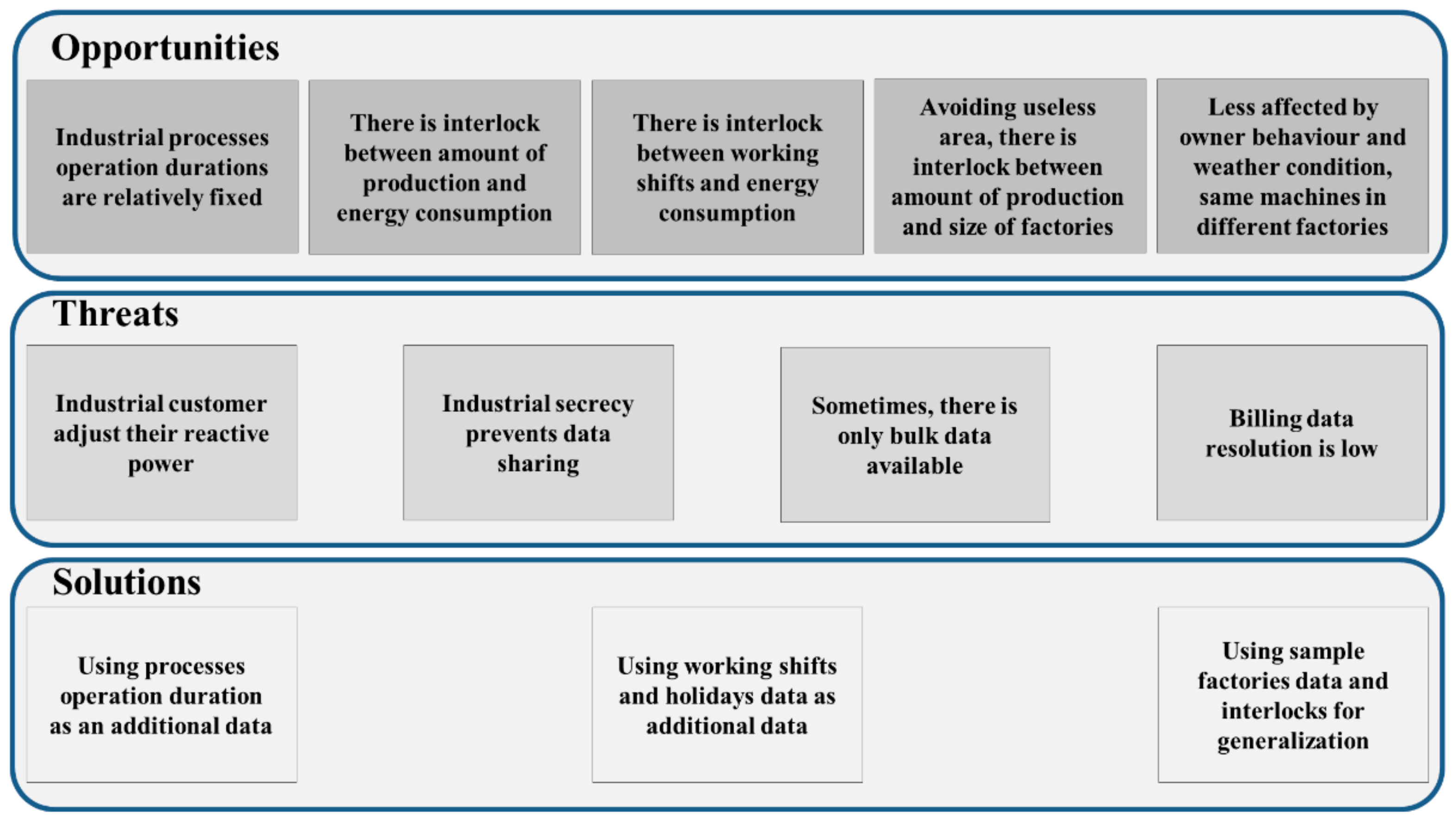
- In contrast to domestic equipment, which typically includes household appliances (e.g., fridge, TV, and washing machines), equipment types vary greatly in different industries [9]. As such, the domestic load disaggregation methods may fail when applied to the industrial sector. This necessitates a unique load analysis for any given industry.
- As there are more diverse load types in the industrial sector than in the domestic sector, the logical assumption of a unique signature for a given load in the ∆P–∆Q plane may not be valid for the industrial user [28]. When there are only active power data available, as there is no ΔQ axis, the risk of having the same points for different appliances is much higher. Hence, load identification accuracy decreases.
- In the industrial sector, electrical energy consumption is not separable from the flow of raw materials, intermediate materials, water, and gas [41]. Moreover, minimum intermediate material storage is important in industries. Thus, the sequence of processes may be considered. As the energy consumption of processes is linked, limits on any form of input energy or water may add constraints to the problem.
- It is difficult, and in some cases impossible, to install smart meters for all houses [42]. Dynamic measurement is much more difficult for the industrial sector. Hence, high-resolution data are not always available to offer disaggregated load information or enable disaggregation calculations.
- Given that factories pay for both active and reactive power consumption, they are motivated to use equipment for power factor adjustment, such as capacitors. As a result, reactive power cannot be used as additional data.
- Industrial secrecy is a severe challenge [9]. Industrial owners are very likely to be unwilling to share data, install meters, and fill diaries. Motivations are even less in countries with low industrial energy prices such as Kuwait [37] and India [35]. In most cases, there are only bulk point data available, which precludes the use of efficient load modelling algorithms such as smart meter-based methods [15,26,43,44,45], appliance feature-based methods [17,19,43,44,45,46,47,48,49], or methods needing training [28,29,50]. Furthermore, the limited methods addressing industrial NILM [27,28,29] may not be useful since they need high-frequency data acquisition.
- In most cases, providers have only bulk point data with low-resolution time steps (e.g., 15 min or more), which are installed for billing purposes. The installation of more accurate equipment is unattractive due to costs. As a consequence, transient state methods ([14,16,50]) become useless in these cases.
- Using industrial process operation duration as additional data in load disaggregation instead of reactive power, current waveform, or other electrical features used in previous studies;
- Using energy consumption–material production and energy consumption–manpower links in industrial load disaggregation;
- Providing acceptable results with low-resolution input data (hourly data in day study horizon).
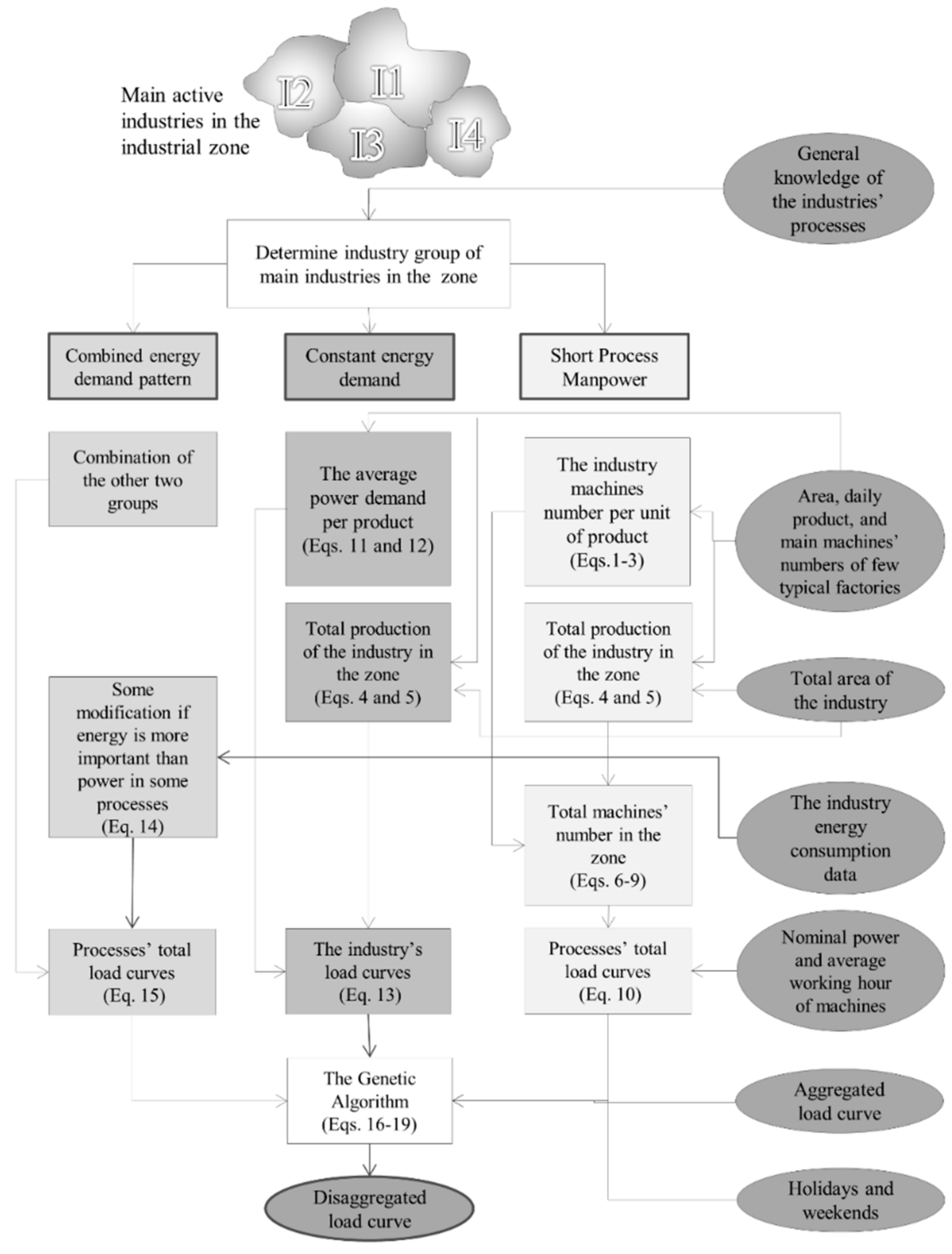
2. Industrial Load Disaggregation Methodology
2.1. Industry Groups
2.1.1. Short Process Manpower (SPM) Industries
- Most processes take a few hours or can be split into a few hours.
- Most processes demand manpower to conduct or supervise the activity (sporadic processes such as slowly warming or cooling materials do not need manpower).
- The energy consumption curves show increases and decreases that can be linked to working shift hours.
- Generate the weekly energy consumption curves (electricity and/or gas).
- Distinguish weekdays and weekends or public holidays, noting that different countries and cultures have different weekends or public holidays. Weekends for industries vary from 0–2 days across the world, often happening from Friday to Sunday. Even within a country, there might be multiple time zones, and different states might have their own public holidays.
- Determine daily shifts. Increases and decreases in the daily energy consumption curve are very helpful in this case.
- Once the working shift schedules are identified, the next step would be the identification of process schedules and their consequent load. The following questions can help at this stage:
- ◦
- Processes taking time more than one working shift: The inquiry here would be to determine whether such processes can split to fit completely in daily working shifts. If so, the start and end times of such processes can be fixed.
- ◦
- A process requiring less time than a full working shift: In such cases, the processes would be assumed to begin sometime after the shift start time to be finished before the end of shifts.
- ◦
- Consider working hour duration. If the process duration is the same as the working hour, there is no need to define the start time. The start time and the end time of the process are the same as daily working hours. If the process duration is less than the working hour duration, the start time is defined so that the process starts and ends during working hours. If the process duration is longer than the working hour duration, the start time may be any time up to 24 h.
2.1.2. Constant Energy Demand (CED) Industries
- Most of the processes are 24/7 activities.
- The energy consumption curves show a “reasonable amount” of load on weekends or public holidays, which implies the continual operation of some processes. The “reasonable amount” implies that the baseload demand is much greater than nonindustrial energy consumption in the zone, for example, lighting energy consumption.
- Form the weekly energy consumption curves (electricity and/or gas).
- Distinguish weekdays and weekends or public holidays.
- Determine the weekly holiday energy consumption. There should not be a significant variation in weekly holiday energy consumption. Otherwise, the industry’s off-days have not been determined correctly.
- Once the working shift schedules are identified, the following questions can help further specify the schedule of processes:
- ◦
- Baseload operations: Identify activities that cannot be stopped even for a short period and consider them constant loads.
- ◦
- Interruptible processes: For a process that can pause their operation, if they are manpower-reliant, they can be assumed to start after shifts start to be finished before the end of shifts. Otherwise, they can have a start time any time within a day (24 h).
2.1.3. Combined Energy Demand Pattern (CEDP) Industries
- The industrial processes include both short and long period activities.
- The energy consumption curves show a reasonable amount of energy consumption difference in weekend and public holiday load, as well as during non-shift hours of weekdays.
- The energy consumption curves show increases and decreases that can be linked to shift hours.
- Determine the difference between the weekly holiday energy consumption and the working day non-shift hours energy consumption. This amount is connected to long period processes. If it is relatively constant, there are 24 h but not 24/7 activities and they are considered fixed consumption during the weekdays. Otherwise, any time within 24 h may be the start time.
2.2. Industry Energy Consumption Evaluation
2.2.1. SPM Industry: Machine-Based (MB) Method
2.2.2. CED Industry: Constant Working Equipment (CWE) Method
2.2.3. CEDP Industry: Combined Energy Usage Pattern (CEUP) Method
2.3. Decomposition Challenges and Solutions
3. Case Studies
3.1. Stonecutting Industry
3.2. Food Industry (Cold Storage)
3.3. Glass Container Industry
3.4. Flat Glass Industry
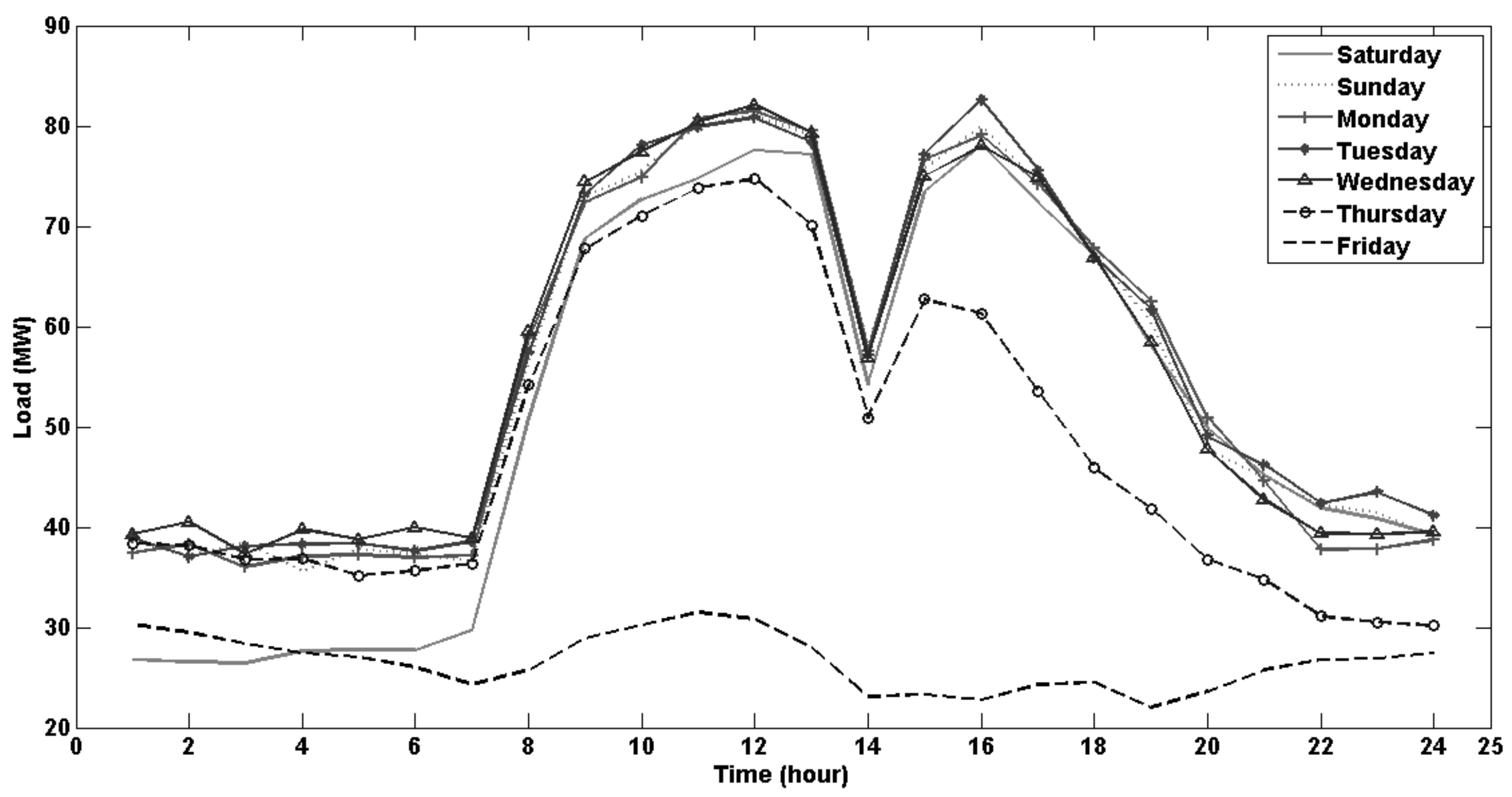
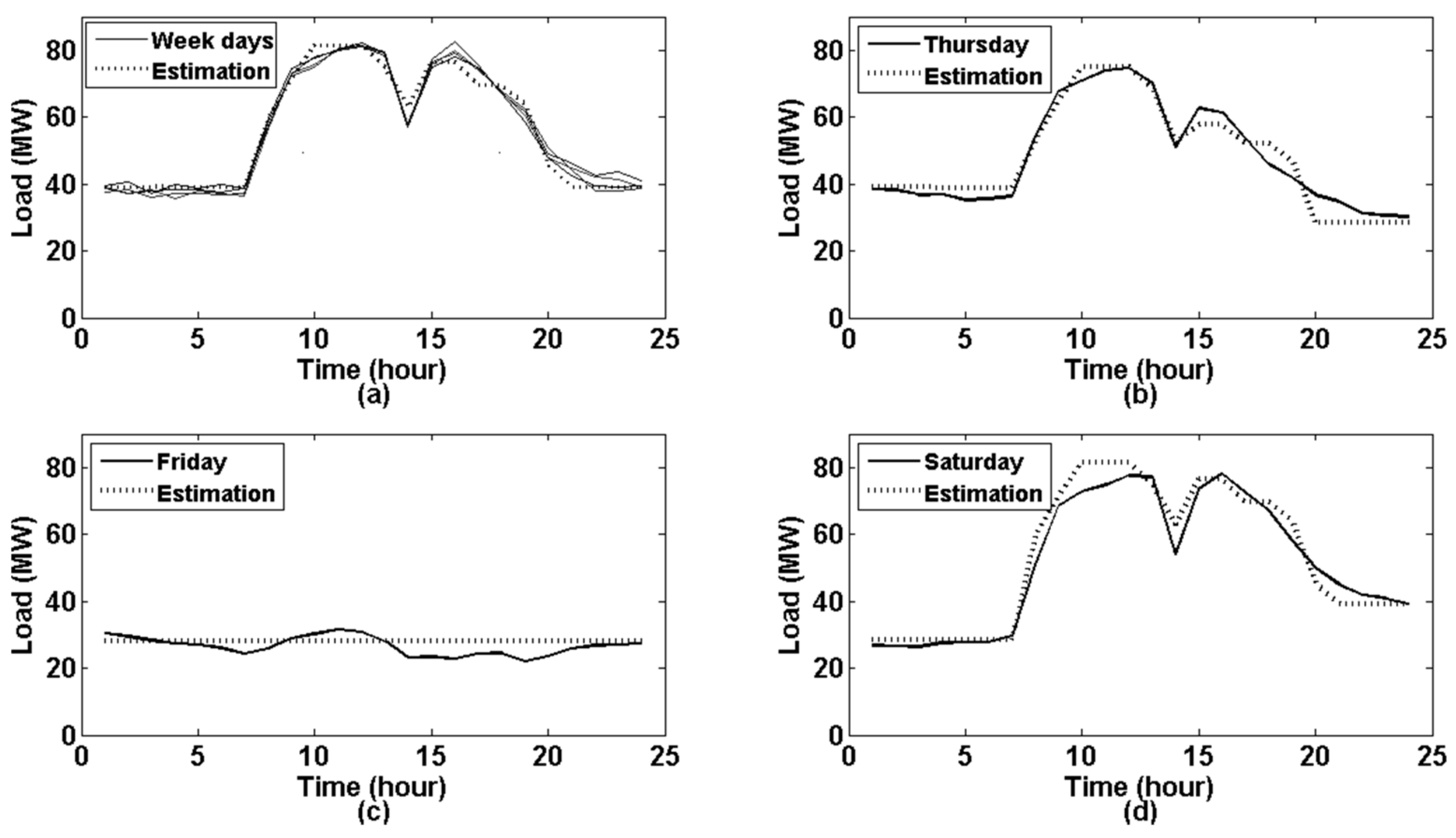
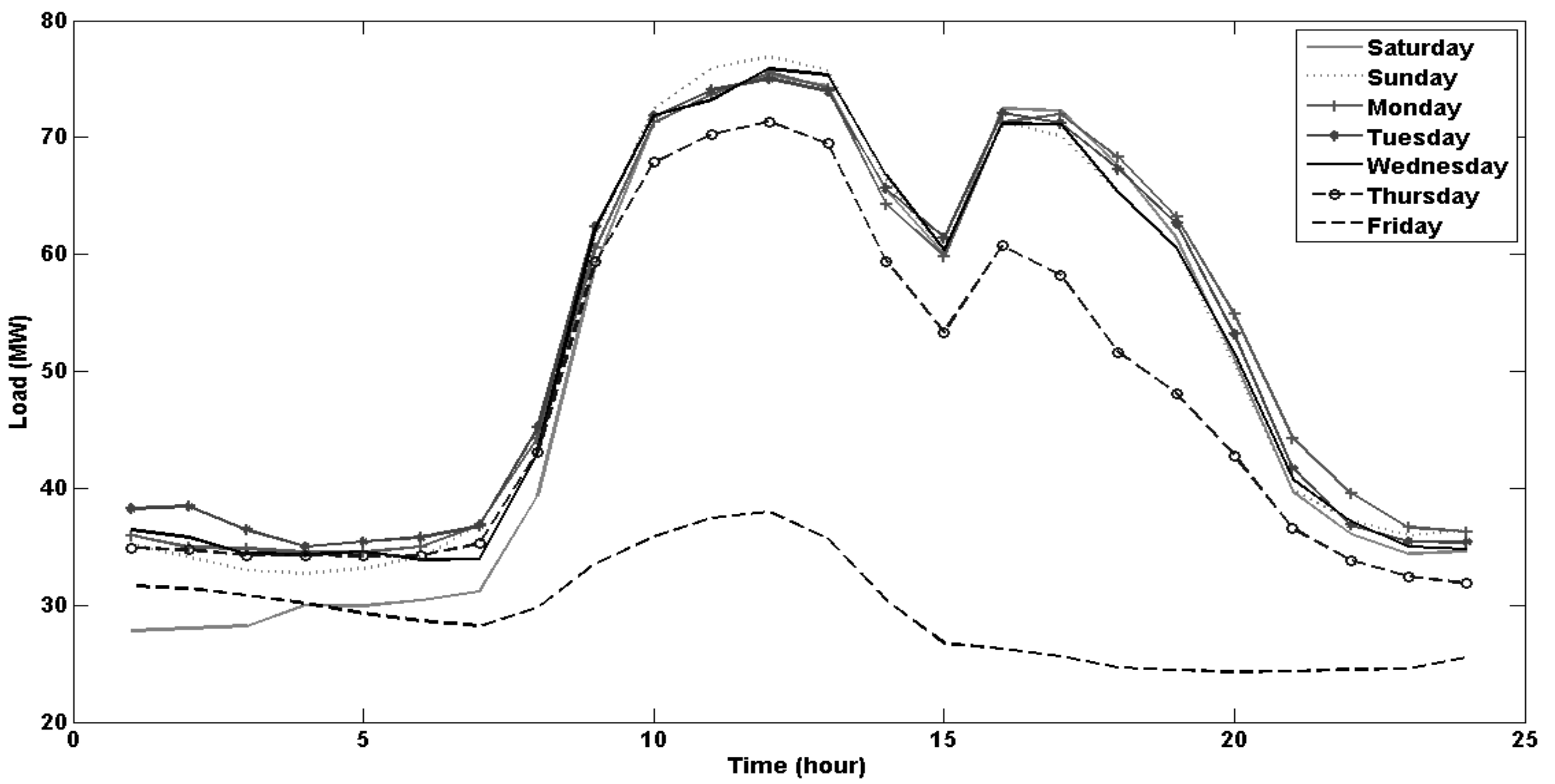
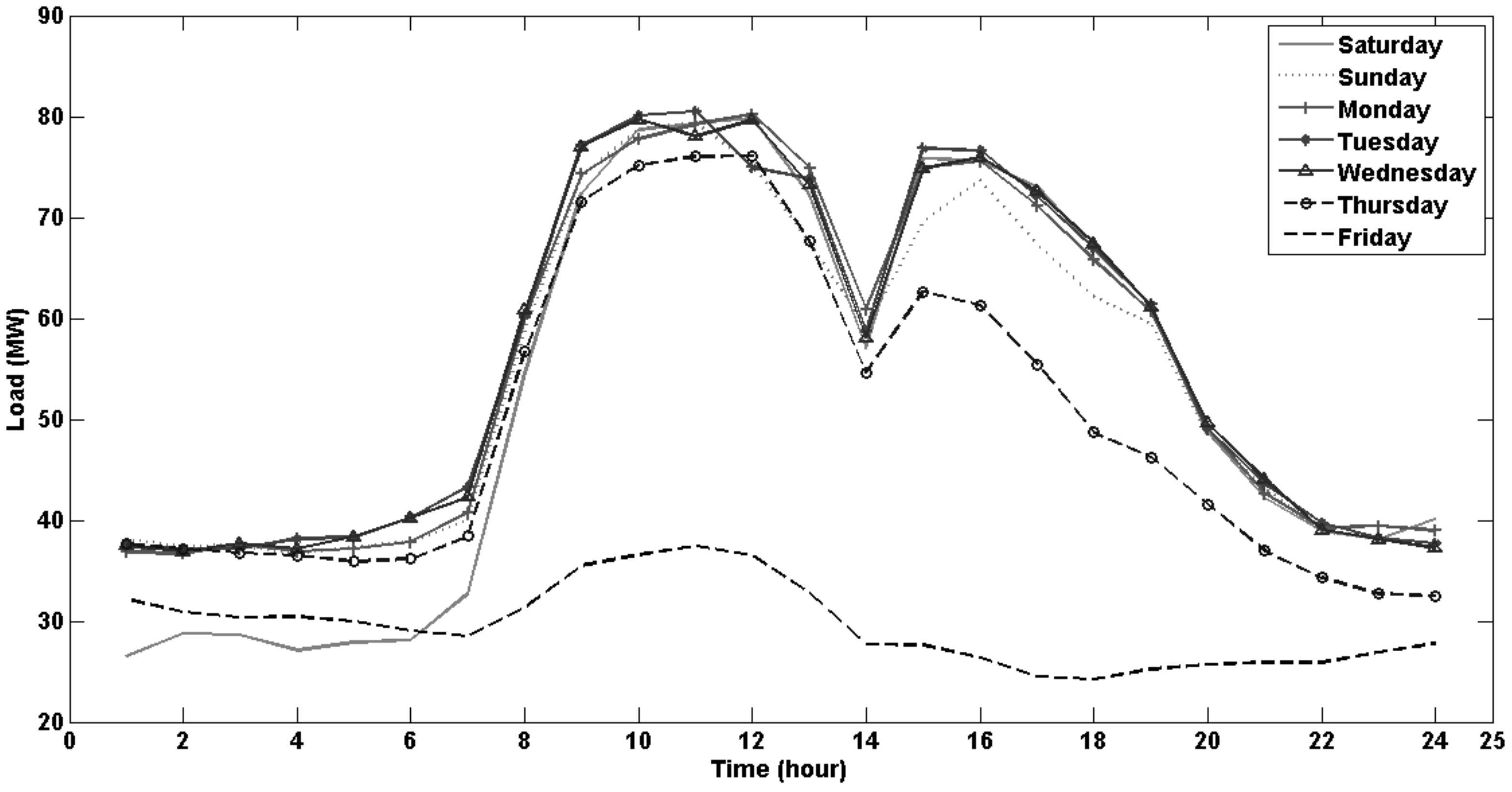
3.5. Decomposition of Load Curves
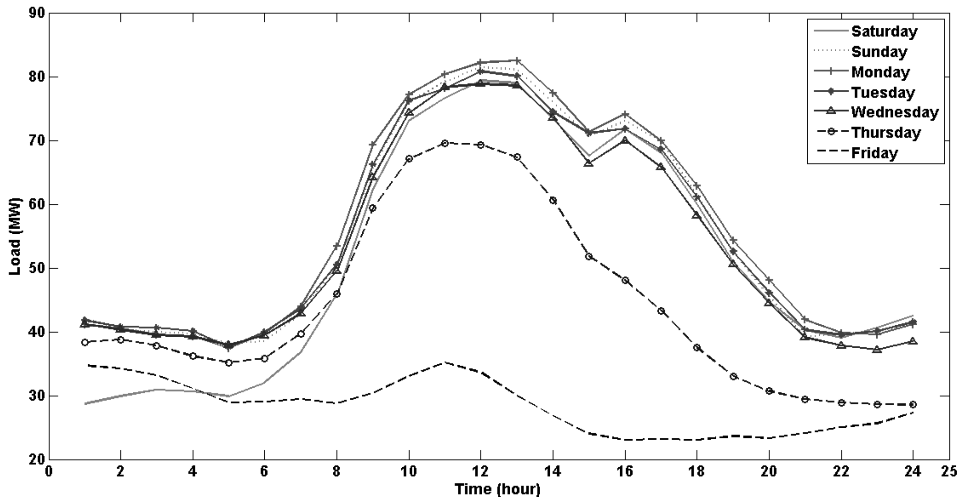
- Friday’s load curve was relatively constant. In Iran, weekends are Thursday and Friday. This was related to a constant load, including glass melting and the cold store’s constant load, which helped in calculating the maximum industry factor for the industries with a constant load.
- Saturday’s load curve until 7 a.m. was similar to Friday’s. Other manpower-demanding processes do not begin until 8 a.m. on the first working day of the week.
- Thursday’s evening load curve implies the inactivity of some industries.
- There were valleys in the load curves from 1–3 p.m. due to the inactivity of manpower-based processes during the lunch break. This separated the working hours into two periods from 9 a.m. to 1 p.m. and from 3 p.m. to 5 p.m. Therefore, it was reasonable to consider stonecutting as a two-part process, instead of an 8 h process.
- The load curves of Sunday to Wednesday were similar, and the average load curve was used to reduce the calculation burden. The average peak load in the week helped to calculate the maximum industry factor for the industries.
- There was a difference between weekend night load and weekday night load. This difference likely resulted from a 24 h process that did not need to continue.
3.5.1. Upper Limits Using the Minimum Value of the Zone’s Load Curve
3.5.2. Upper Limits Using the Maximum Value of the Zone’s Load Curve
3.5.3. Upper Limits Using Curve Characteristics
3.5.4. Lower Limits Using the Maximum Value of the Zone’s Load Curve
4. Results
5. Discussion and Conclusions
Author Contributions
Funding
Institutional Review Board Statement
Informed Consent Statement
Data Availability Statement
Conflicts of Interest
Nomenclatures
| a | On or off state {0,1} |
| A | Area |
| Average area | |
| B | Start time of the process |
| e | Energy per unit of product |
| i | Machine/equipment/process |
| Industry factor | |
| j | Factory |
| k | Industry |
| m | Per-unit number of machines |
| M | Number of machines/equipment |
| Number of sample factories | |
| Total number of factories | |
| p | Rated power of machine/equipment |
| P | Total power |
| Estimated load | |
| pr | Daily product |
| Average product per unit of area | |
| T | Time duration |
| t | Hour |
References
- Zhao, L.; Zhou, Y.; Quilumba, F.L.; Lee, W.J. Potential of the Commercial Sector to Participate in the Demand Side Management Program. In Proceedings of the IEEE Transactions on Industry Applications; Institute of Electrical and Electronics Engineers Inc.: Piscataway, NJ, USA, 26 August, 2019; Volume 55, pp. 7261–7269. [Google Scholar] [CrossRef]
- Zhang, Q.; Grossmann, I.E. Enterprise-wide optimization for industrial demand side management: Fundamentals, advances, and perspectives. Chem. Eng. Res. Des. 2016, 116, 114–131. [Google Scholar] [CrossRef] [Green Version]
- Company, Iran Grid Management Report on the Status of the Country’s Electricity Transmission Network. 2020.
- Strbac, G. Demand side management: Benefits and challenges. Energy Policy 2008, 36, 4419–4426. [Google Scholar] [CrossRef]
- Zhang, Q.; Grossmann, I.E. Planning and scheduling for industrial demand side management: Advances and challenges. In Alternative Energy Sources and Technologies: Process Design and Operation; Springer International Publishing: New York, NY, USA, 2016; pp. 383–414. ISBN 9783319287522. [Google Scholar]
- Khan, I.; Jack, M.W.; Stephenson, J. Dominant factors for targeted demand side management—An alternate approach for residential demand profiling in developing countries. Sustain. Cities Soc. 2021, 67, 102693. [Google Scholar] [CrossRef]
- Tawalbeh, N.; Abusamaha, H.M.; Al-Salaymeh, A. Demand side management and its possibilities in jordan. J. Ecol. Eng. 2020, 21, 29–33. [Google Scholar] [CrossRef]
- Samad, T.; Kiliccote, S. Smart grid technologies and applications for the industrial sector. Comput. Chem. Eng. 2012, 47, 76–84. [Google Scholar] [CrossRef]
- Adabi, A.; Mantey, P.; Holmegaard, E.; Kjaergaard, M.B. Status and challenges of residential and industrial non-intrusive load monitoring. In Proceedings of the 2015 IEEE Conference on Technologies for Sustainability, SusTech 2015, Ogden, UT, USA, 30 July–1 August 2015; Institute of Electrical and Electronics Engineers Inc.: Piscataway, NJ, USA, 2015; pp. 181–188. [Google Scholar] [CrossRef]
- Cardoso, C.A.; Torriti, J.; Lorincz, M. Making demand side response happen: A review of barriers in commercial and public organisations. Energy Res. Soc. Sci. 2020, 64, 101443. [Google Scholar] [CrossRef]
- Castro, P.M.; Ave, G.D.; Engell, S.; Grossmann, I.E.; Harjunkoski, I. Industrial Demand Side Management of a Steel Plant Considering Alternative Power Modes and Electrode Replacement. Ind. Eng. Chem. Res. 2020, 59, 13642–13656. [Google Scholar] [CrossRef]
- Gaur, M.; Majumdar, A. Disaggregating transform learning for non-intrusive load monitoring. IEEE Access 2018, 6, 46256–46265. [Google Scholar] [CrossRef]
- Hart, G.W. Nonintrusive Appliance Load Monitoring. Proc. IEEE 1992, 80, 1870–1891. [Google Scholar] [CrossRef]
- Norford, L.K.; Leeb, S.B. Non-intrusive electrical load monitoring in commercial buildings based on steady-state and transient load-detection algorithms. Energy Build. 1996, 24, 51–64. [Google Scholar] [CrossRef]
- Farinaccio, L.; Zmeureanu, R. Using a pattern recognition approach to disaggregate the total electricity consumption in a house into the major end-uses. Energy Build. 1999, 30, 245–259. [Google Scholar] [CrossRef]
- Chang, H.H.; Chen, K.L.; Tsai, Y.P.; Lee, W.J. A new measurement method for power signatures of nonintrusive demand monitoring and load identification. In Proceedings of the IEEE Transactions on Industry Applications; IEEE: Piscataway, NJ, USA, 2012; Volume 48, pp. 764–771. [Google Scholar]
- Liang, J.; Ng, S.K.K.; Kendall, G.; Cheng, J.W.M. Load signature studypart I: Basic concept, structure, and methodology. IEEE Trans. Power Deliv. 2010, 25, 551–560. [Google Scholar] [CrossRef]
- Devlin, M.A.; Hayes, B.P. Load identification and classification of activities of daily living using residential smart meter data. In Proceedings of the 2019 IEEE Milan PowerTech, PowerTech 2019, Politecnico di Milano, Milan, Italy, 23–27 June 2019; Institute of Electrical and Electronics Engineers Inc.: Piscataway, NJ, USA, 2019. [Google Scholar] [CrossRef]
- Baranski, M.; Voss, J. Genetic algorithm for pattern detection in NIALM systems. In Proceedings of the International Conference on Systems, Man and Cybernetics, Hague, The Netherlands, 10–13 October 2004; Volume 4, pp. 3462–3468. [Google Scholar]
- Suzuki, K.; Inagaki, S.; Suzuki, T.; Nakamura, H.; Ito, K. Nonintrusive appliance load monitoring based on integer programming. In Proceedings of the SICE Annual Conference, Tokyo, Japan, 20–22 August 2008; pp. 2742–2747. [Google Scholar]
- Liang, J.; Ng, S.K.K.; Kendall, G.; Cheng, J.W.M. Load signature studypart II: Disaggregation framework, simulation, and applications. IEEE Trans. Power Deliv. 2010, 25, 561–569. [Google Scholar] [CrossRef]
- Green, D.H.; Shaw, S.R.; Lindahl, P.; Kane, T.J.; Donnal, J.S.; Leeb, S.B. A MultiScale Framework for Nonintrusive Load Identification. IEEE Trans. Ind. Inform. 2020, 16, 992–1002. [Google Scholar] [CrossRef]
- Zeifman, M.; Roth, K. Disaggregation of home energy display data using probabilistic approach. In Proceedings of the Digest of Technical Papers—IEEE International Conference on Consumer Electronics, Las Vegas, NV, USA, 12–15 January 2012; pp. 630–631. [Google Scholar] [CrossRef]
- Zoha, A.; Gluhak, A.; Imran, M.; Rajasegarar, S. Non-Intrusive Load Monitoring Approaches for Disaggregated Energy Sensing: A Survey. Sensors 2012, 12, 16838–16866. [Google Scholar] [CrossRef] [Green Version]
- Esa, N.F.; Abdullah, M.P.; Hassan, M.Y. A review disaggregation method in Non-intrusive Appliance Load Monitoring. Renew. Sustain. Energy Rev. 2016, 66, 163–173. [Google Scholar] [CrossRef]
- Carrie Armel, K.; Gupta, A.; Shrimali, G.; Albert, A. Is disaggregation the holy grail of energy efficiency? The case of electricity. Energy Policy 2013, 52, 213–234. [Google Scholar] [CrossRef] [Green Version]
- Batra, N.; Parson, O.; Berges, M.; Singh, A.; Rogers, A. A Comparison of Non-Intrusive Load Monitoring Methods for Commercial and Residential Buildings. August 2014. Available online: http://arxiv.org/abs/1408.6595 (accessed on 24 December 2020).
- Laughman, C.; Lee, K.; Cox, R.; Shaw, S.; Leeb, S.; Norford, L.; Armstrong, P. Power signature analysis. IEEE Power Energy Mag. 2003, 1, 56–63. [Google Scholar] [CrossRef]
- Chang, H.H.; Yang, H.T.; Lin, C.L. Load identification in neural networks for a non-intrusive monitoring of industrial electrical loads. In Proceedings of the Lecture Notes in Computer Science (Including Subseries Lecture Notes in Artificial Intelligence and Lecture Notes in Bioinformatics), Karlsruhe, Germany, 15–17 September 2008; Springer: Berlin/Heidelberg, Germany, 2008; Volume 5236, pp. 664–674. [Google Scholar] [CrossRef]
- Martins, P.B.M.; Gomes, J.G.R.C.; Nascimento, V.B.; De Freitas, A.R. Application of a Deep Learning Generative Model to Load Disaggregation for Industrial Machinery Power Consumption Monitoring. In Proceedings of the 2018 IEEE International Conference on Communications, Control, and Computing Technologies for Smart Grids (SmartGridComm), Aalborg, Denmark, 29–31 October 2018. [Google Scholar] [CrossRef]
- Brucke, K.; Arens, S.; Telle, J.-S.; Von Maydell, K.; Agert, C. Particle Swarm Optimization for Energy Disaggregation in Industrial and Commercial Buildings. arXiv 2020, arXiv:2006.12940. [Google Scholar]
- Yang, F.; Liu, B.; Luan, W.; Zhao, B.; Liu, Z.; Xiao, X.; Zhang, R. FHMM Based Industrial Load Disaggregation. In Proceedings of the 2021 6th Asia Conference on Power and Electrical Engineering (ACPEE), Chongqing, China, 8–11 April 2021; pp. 330–334. [Google Scholar] [CrossRef]
- Yang, M. Demand side management in Nepal. Energy 2006, 31, 2677–2698. [Google Scholar] [CrossRef]
- Paulus, M.; Borggrefe, F. The potential of demand-side management in energy-intensive industries for electricity markets in Germany. Appl. Energy 2011, 88, 432–441. [Google Scholar] [CrossRef]
- Harish, V.S.K.V.; Kumar, A. Demand side management in India: Action plan, policies and regulations. Renew. Sustain. Energy Rev. 2014, 33, 613–624. [Google Scholar] [CrossRef]
- Warren, P. A review of demand-side management policy in the UK. Renew. Sustain. Energy Rev. 2014, 29, 941–951. [Google Scholar] [CrossRef]
- Alasseri, R.; Tripathi, A.; Joji Rao, T.; Sreekanth, K.J. A review on implementation strategies for demand side management (DSM) in Kuwait through incentive-based demand response programs. Renew. Sustain. Energy Rev. 2017, 77, 617–635. [Google Scholar] [CrossRef]
- Omar, S.A.S. Kuwait Energy Outlook. 2019. Available online: https://www.undp.org/content/dam/rbas/doc/Energy%20and%20Environment/KEO_report_English.pdf (accessed on 6 August 2021).
- Zhang, S.; Jiao, Y.; Chen, W. Demand-side management (DSM) in the context of China’s on-going power sector reform. Energy Policy 2017, 100, 1–8. [Google Scholar] [CrossRef]
- IEA. Demand Response; IEA: Paris, France, 2020; Available online: https://www.iea.org/reports/demand-response (accessed on 6 August 2021).
- Ding, Y.M.; Hong, S.H.; Li, X.H. A demand response energy management scheme for industrial facilities in smart grid. IEEE Trans. Ind. Inform. 2014, 10, 2257–2269. [Google Scholar] [CrossRef]
- Xu, Y.; Milanović, J.V. Artificial-intelligence-based methodology for load disaggregation at bulk supply point. IEEE Trans. Power Syst. 2015, 30, 795–803. [Google Scholar] [CrossRef]
- Cominola, A.; Giuliani, M.; Piga, D.; Castelletti, A.; Rizzoli, A.E. A Hybrid Signature-based Iterative Disaggregation algorithm for Non-Intrusive Load Monitoring. Appl. Energy 2017, 185, 331–344. [Google Scholar] [CrossRef]
- He, K.; Stankovic, L.; Liao, J.; Stankovic, V. Non-Intrusive Load Disaggregation Using Graph Signal Processing. IEEE Trans. Smart Grid 2018, 9, 1739–1747. [Google Scholar] [CrossRef] [Green Version]
- Hock, D.; Kappes, M.; Ghita, B. Non-Intrusive Appliance Load Monitoring using Genetic Algorithms. In Proceedings of the IOP Conference Series: Materials Science and Engineering, Kuala Lumpur, Malaysia, 13–14 August 2018; Institute of Physics Publishing: Bristol, UK, 2018; Volume 366, p. 012003. [Google Scholar] [CrossRef]
- Zeifman, M.; Roth, K. Nonintrusive appliance load monitoring: Review and outlook. IEEE Trans. Consum. Electron. 2011, 57, 76–84. [Google Scholar] [CrossRef]
- Figueiredo, M.; de Almeida, A.; Ribeiro, B. Home electrical signal disaggregation for non-intrusive load monitoring (NILM) systems. Neurocomputing 2012, 96, 66–73. [Google Scholar] [CrossRef]
- Belley, C.; Gaboury, S.; Bouchard, B.; Bouzouane, A. An efficient and inexpensive method for activity recognition within a smart home based on load signatures of appliances. In Proceedings of the Pervasive and Mobile Computing; Elsevier B.V.: Amsterdam, The Netherlands, 2014; Volume 12, pp. 58–78. [Google Scholar] [CrossRef] [Green Version]
- Deb, C.; Frei, M.; Hofer, J.; Schlueter, A. Automated load disaggregation for residences with electrical resistance heating. Energy Build. 2019, 182, 61–74. [Google Scholar] [CrossRef]
- Patel, S.N.; Robertson, T.; Kientz, J.A.; Reynolds, M.S.; Abowd, G.D. At the Flick of a Switch: Detecting and Classifying Unique Electrical Events on the Residential Power Line (Nominated for the Best Paper Award). In UbiComp 2007: Ubiquitous Computing; Springer: Berlin/Heidelberg, Germany, 2007; pp. 271–288. [Google Scholar]
- Mohseni, S.; Haratian, M. Energy audit and estimation of electricity consumption criteria in stone cutting plants. In Proceedings of the 24th Power System Conference, Tehran, Iran, 16 November 2009; Available online: https://civilica.com/doc/89372/ (accessed on 6 August 2021).
- Gharechahi, H.; Askari, M. Design of energy consumption optimization system for stonecutting plants’ polishing machines. In Proceedings of the National Conference of Mechanical Engineering Iran, Shiraz, Iran, 27 February 2014; Available online: https://civilica.com/doc/247819/ (accessed on 6 August 2021).
- Ruth, M.; Dell’Anno, P. An industrial ecology of the US glass industry. Resour. Policy 1997, 23, 109–124. [Google Scholar] [CrossRef]
- Lawrence, A.; Thollander, P.; Andrei, M.; Karlsson, M. Specific Energy Consumption/Use (SEC) in Energy Management for Improving Energy Efficiency in Industry: Meaning, Usage and Differences. Energies 2019, 12, 247. [Google Scholar] [CrossRef] [Green Version]
- Glass the industry of future 2002. Available online: https://www.nrel.gov/docs/fy02osti/32135.pdf (accessed on 24 December 2020).
- Manufacturing Energy and Carbon Footprints (2014 MECS. Department of Energy. Available online: https://www.energy.gov/eere/amo/manufacturing-energy-and-carbon-footprints-2014-mecs (accessed on 24 December 2020).


| Study | Case Study | Variables | Sample Rate (Hz) |
|---|---|---|---|
| Laughman et al. [28] | An industrial building | The active and reactive power | 8000 |
| Chang et al. [29] | An industrial building | The voltage and current waveforms in a three-phase electrical service | 15,000 |
| Martins et al. [30] | One factory | The active power | 1 |
| Brucke et al. [31] | An industrial building | The active and reactive power | 1 |
| Yang et al. [32] | One factory | The active and reactive power | 1 |
| Processes Take a Few Hours or Can Be Split into a Few Hours | Processes Are 24/7 Activities | Processes Demand Manpower | The Energy Consumption Curves Show Increases and Decreases Linked to Working Shift Hours | The Energy Consumption Curves Show Energy Consumption on Weekends and Off-Days | |
|---|---|---|---|---|---|
| SPM | ✓ | ✕ | ✓ | ✓ | ✕ |
| CED | ✕ | ✓ | ✕ | ✕ | ✓ |
| CEDP | ✓ | ✓ | ✓ | ✓ | ✓ |
| Manufacturer | Block Cutting (No.) | Polishing Machine (No.) | Length Cutting Machine (No.) | Width Cutting Machine (No.) | Width | ||
|---|---|---|---|---|---|---|---|
| 1 | 300 | 2 | 6.67 | 1 | 1 | 3 | 10 |
| 2 | 200 | 2 | 10 | 1 | 1 | 2 | 10 |
| 3 | 250 | 2 | 8 | 1 | 1 | 1 | 4 |
| 4 | 300 | 3 | 10 | 1 | 1 | 2 | 6.67 |
| 5 | 120 | 1 | 8.33 | 1 | 1 | 1 | 8.33 |
| 6 | 100 | 1 | 10 | 1 | 1 | 2 | 20 |
| 7 | 130 | 2 | 15.4 | 1 | 1 | 1 | 7.7 |
| 8 | 200 | 1 | 5 | 1 | 1 | 1 | 5 |
| 9 | 100 | 1 | 10 | 1 | 1 | 2 | 20 |
| 10 | 110 | 1 | 9.1 | 1 | 1 | 1 | 9.1 |
| Manufacturer | Daily Product (m2/day) | Area (Aj,s) (ha) | Per-Unit Daily Product (prj,s) (m2/(day·ha)) |
|---|---|---|---|
| 1 | 2092 | 2 | 1046 |
| 2 | 418.12 | 2.3 | 181.79 |
| 3 | 125.42 | 0.5 | 250.87 |
| 4 | 125.43 | 0.5 | 250.87 |
| Machine | Average Power (kW) | Daily Working Hours (h/day) |
|---|---|---|
| Block cutting machine | 110 | 24 |
| Polishing machine | 11 | 8 |
| Length-cutting | 30 | 8 |
| Width-cutting | 4 | 8 |
| Other machines | 80 | 1–24 (considering the machine) |
| Machine | Average Power (MW) | Daily Working Hours (h/day) |
|---|---|---|
| Block cutting machine | 730.73 | 24 |
| Polishing machine | 7.304 | 8 |
| Length-cutting | 19.92 | 8 |
| Width-cutting | 2.656 | 8 |
| Other machines | 53.12 | 12 |
| Food Industry Load | Average Power (MW) | Daily Working Hours (h/day) |
|---|---|---|
| Constant load | 1175.6 | 24 |
| Variable load | 13.37 | 8 |
| Manufacturer | Daily Product 1 (tonne/day) | Area (ha) | Per-Unit Daily Product (tonne/(day·ha)) |
|---|---|---|---|
| Nouri Taze | 183 | 72 | 2.55 |
| 2 | 237 | 49.2 | 4.81 |
| 3 | 65 | 9 | 7.20 |
| 4 | 250 | 40 | 6.25 |
| Process | Average Specific Energy Use 1 (106 Btu/tonne) | Average Specific Electricity Use 1 (106 Btu/tonne) | Rated Power (MW/tonne) 1 | Total Power (MW) | Process Duration (hr) |
|---|---|---|---|---|---|
| Batching | 0.27–1.2 | 0.53 | 0.0388 | 57.14 | 4 |
| Melting | 5.5 | 0.825 | 0.0101 | 14.88 | 24 |
| Forming | 0.4 | 0.4 2 | 0.0195 | 28.72 | 6 |
| Post-Forming | 1.86 | 0.23 | 0.0169 | 24.89 | 4 |
| Manufacturer | Daily Product 1 (tonne/day) | Area (ha) | Per-Unit Daily Product (tonne/(day·ha)) |
|---|---|---|---|
| 1 | 900 | 75 | 12 |
| 2 | 200 | 1.8 | 114.3 |
| 3 | 400 | 30 | 13.3 |
| Process | Average Specific Energy Use 1 (106 Btu/tonne) | Average Specific Electricity Use 1 (106 Btu/tonne) | Rated Power (MW/tonne) 1 | Total Power (MW) | Process Duration (h) |
|---|---|---|---|---|---|
| Batching | 0.27–1.2 | 0.27 | 0.0198 | 101.44 | 4 |
| Melting 2 | 6.5 | 0.845 | 0.0103 | 52.91 | 24 |
| Forming 3 | 1.5 | 1.5 | 0.0366 | 187.85 | 12 |
| Post-Forming 4 | 2.06 | 0.15 | 0.0110 | 56.36 | 4 |
| Industry | Flat Glass Industry | Glass Container Industry | Food Industry | Stonecutting Industry |
|---|---|---|---|---|
| Maximum IF | 0.2542 | 0.2875 | 0.0226 | 0.0156 |
| Minimum IF | - | 0.0212 | - | - |
| Industry | Process | Duration | Start Time Lower Limit | Start Time Upper Limit |
|---|---|---|---|---|
| Flat glass | Batching | 4 | 8 | 17 |
| Forming | 12 | 1 | 9 | |
| Post-forming | 4 | 8 | 17 | |
| Glass container | Batching | 4 | 8 | 17 |
| Forming | 6 | 8 | 15 | |
| Post-forming | 4 | 8 | 17 | |
| Food industry | forklifts | 8 | 16 | 29 |
| Variables | Results for Various Weekdays | |||
|---|---|---|---|---|
| Sunday–Wednesday | Thursday | Friday | Saturday | |
| Flat glass industry factor | 0.0998 | 0.0992 | 0.0992 | 0.0998 |
| Glass container industry factor | 0.2114 | 0.2110 | 0.2110 | 0.2114 |
| Stonecutting industry factor 1 | 0.0147 | 0.0000 | 0.0000 | 0.01471 |
| Food industry factor | 0.0169 | 0.0168 | 0.0168 | 0.0169 |
| Batching, flat glass start time (h) | 10 | 10 | - | 10 |
| Forming, flat glass start time (h) | 8 | 8 | - | 8 |
| Post forming, flat glass start time (h) | 15 | 13 | - | 15 |
| Batching, glass container start time (h) | 9 | 9 | - | 9 |
| Forming, glass container start time (h) | 15 | 8 | - | 15 |
| Post forming, glass container start time (h) | 13 | 15 | - | 13 |
| Forklifts, food start time (h) | 20 | 20 | - | 20 |
| Estimation error (%) | 4.83 | 7.1 | 11.56 | 7.82 |
| Variables | Results for Various Weekdays | |||
|---|---|---|---|---|
| Sunday–Wednesday | Thursday | Friday | Saturday | |
| Flat glass industry factor | 0.0691 | 0.0653 | 0.0653 | 0.0691 |
| Glass container industry factor | 0.2752 | 0.2750 | 0.2750 | 0.2752 |
| Stonecutting industry factor 1 | 0.0150 | 0.0000 | 0.0000 | 0.0150 * |
| Food industry factor | 0.0184 | 0.0170 | 0.0170 | 0.0184 |
| Batching, flat glass start time (h) | 14 | 14 | - | 14 |
| Forming, flat glass start time (h) | 8 | 8 | - | 8 |
| Post forming, flat glass start time (h) | 13 | 12 | - | 13 |
| Batching, glass container start time (h) | 10 | 10 | - | 10 |
| Forming, glass container start time (h) | 9 | 9 | - | 9 |
| Post forming, glass container start time (h) | 15 | 8 | - | 15 |
| Forklifts, food start time (h) | 20 | 20 | - | 20 |
| Estimation error (%) | 3.62% | 5.45% | 10.51% | 3.41% |
| Variables | Results for Various Weekdays | |||
|---|---|---|---|---|
| Sunday-Wed | Thursday | Friday | Saturday | |
| Flat glass industry factor | 0.0958 | 0.0956 | 0.0956 | 0.0958 |
| Glass container industry factor | 0.1891 | 0.1885 | 0.1885 | 0.1891 |
| Stonecutting industry factor 1 | 0.0111 | 0 | 0 | 0.0111 |
| Food industry factor | 0.0172 | 0.0172 | 0.0172 | 0.0172 |
| Batching, flat glass start time (h) | 10 | 10 | - | 10 |
| Forming, flat glass start time (h) | 9 | 9 | - | 9 |
| Post forming, flat glass start time (h) | 14 | 11 | - | 14 |
| Batching, glass container start time (h) | 16 | 8 | - | 16 |
| Forming, glass container start time (h) | 8 | 12 | - | 8 |
| Post forming, glass container start time (h) | 11 | 16 | - | 11 |
| Forklifts, food start time (h) | 5 | 5 | - | 5 |
| Estimation error (%) | 3.1% | 6.81% | 15.09% | 3.69% |
| Variables | Results for Various Weekdays | |||
| Sunday–Wednesday | Thursday | Friday | Saturday | |
| Flat glass industry factor | 0.0881 | 0.0875 | 0.0875 | 0.0881 |
| Glass container industry factor | 0.2313 | 0.2309 | 0.2309 | 0.2313 |
| Stonecutting industry factor 1 | 0.0144 | 0.0000 | 0.0000 | 0.0144 |
| Food industry factor | 0.0177 | 0.0177 | 0.0177 | 0.0177 |
| Batching, flat glass start time (h) | 10 | 10 | - | 10 |
| Forming, flat glass start time (h) | 8 | 8 | - | 8 |
| Post forming, flat glass start time (h) | 13 | 13 | - | 13 |
| Batching, glass container start time (h) | 9 | 9 | - | 9 |
| Forming, glass container start time (h) | 15 | 12 | - | 15 |
| Post forming, glass container start time (h) | 15 | 8 | - | 15 |
| Forklifts, food start time (h) | 5 | 5 | - | 5 |
| Estimation error (%) | 3.7% | 8.94% | 13.21% | 3.63% |
Publisher’s Note: MDPI stays neutral with regard to jurisdictional claims in published maps and institutional affiliations. |
© 2021 by the authors. Licensee MDPI, Basel, Switzerland. This article is an open access article distributed under the terms and conditions of the Creative Commons Attribution (CC BY) license (https://creativecommons.org/licenses/by/4.0/).
Share and Cite
Tavakoli, S.; Khalilpour, K. A Practical Load Disaggregation Approach for Monitoring Industrial Users Demand with Limited Data Availability. Energies 2021, 14, 4880. https://doi.org/10.3390/en14164880
Tavakoli S, Khalilpour K. A Practical Load Disaggregation Approach for Monitoring Industrial Users Demand with Limited Data Availability. Energies. 2021; 14(16):4880. https://doi.org/10.3390/en14164880
Chicago/Turabian StyleTavakoli, Sara, and Kaveh Khalilpour. 2021. "A Practical Load Disaggregation Approach for Monitoring Industrial Users Demand with Limited Data Availability" Energies 14, no. 16: 4880. https://doi.org/10.3390/en14164880
APA StyleTavakoli, S., & Khalilpour, K. (2021). A Practical Load Disaggregation Approach for Monitoring Industrial Users Demand with Limited Data Availability. Energies, 14(16), 4880. https://doi.org/10.3390/en14164880