Fault Diagnosis of Electric Motors Using Deep Learning Algorithms and Its Application: A Review

Abstract

Electric motors are used extensively in numerous industries, and their failure can result not only in machine damage but also a slew of other issues, such as financial loss, injuries, etc. As a result, there is a significant scope to use robust fault diagnosis technology. In recent years, interesting research results on fault diagnosis for electric motors have been documented. Deep learning in the fault detection of electric equipment has shown comparatively better results than traditional approaches because of its more powerful and sophisticated feature extraction capabilities. This paper covers four traditional types of deep learning models: deep belief networks (DBN), autoencoders (AE), convolutional neural networks (CNN), and recurrent neural networks (RNN), and highlights their use in detecting faults of electric motors. Finally, the issues and obstacles that deep learning encounters in the fault detection mechanism as well as the prospects are discussed and summarized.

1. Introduction

The electric induction motor is perhaps the most significant driver of today’s production activities and everyday life, and it is extensively utilized in many sectors of production and manufacturing industries as well as in domestic utility applications. An electric motor is a mechanical mechanism that transforms electrical energy. Most electric motors work by generating force in the form of torque delivered to the motor’s shaft by interacting between the magnetic field of the motor and the electric current in a wire winding. The failure or stoppage of this type of vital electrical machine will not only harm the equipment itself but will also likely result in significant economic losses, fatalities, pollution, and numerous other issues. Therefore, research into motor fault diagnostic technology is extremely important.

The fault diagnostic technology can detect motor defects early in their development, allowing for prompt overhauls, saving time and money on fault repairs, and enhancing the economic advantages while avoiding production interruptions. Traditional fault diagnostic approaches need the artificial extraction of a considerable quantity of feature data, such as time domain features, frequency domain features, and time–frequency domain features [1,2,3], which adds to the fault diagnostic uncertainty and complexity. Traditional fault diagnosis methods are unable to meet the needs of the fault diagnosis in the context of big data due to the complex and efficient development of motors, which presents the data reflecting the operating status of motors with the characteristics of massive, diversified, fast flowing speed, and low value density of “big data” [4,5,6]. Simultaneously, the advancement of artificial intelligence technology encourages the evolution of fault diagnosis technology from traditional to intelligent [7]. Artificial neural networks (ANNs) were first introduced in the 1980s. Shallow neural networks may learn features in an adaptable manner without creating exact mathematical models [8], eliminating the uncertainty and complexity that human involvement brings. However, traditional shallow neural networks have drawbacks, including gradient vanishing problems, overfitting, local minima, and the requirement for extensive prior information, all of which decrease the effectiveness of the fault diagnosis [9].

In 2006, Hinton et al. [10] developed the concept of deep learning (DL) and demonstrated that data characteristics generated by a deep multilayer network structure may more accurately represent the original data, and that the approach can effectively minimize the complexity of training deep neural networks. This has resulted in a surge in deep learning related research in both academia and industry. In 2007, Bengio et al. [11] suggested the use of unsupervised greedy layer-wise training to train deep neural networks so to optimize the structure of deep networks parameters in order to improve the model generalization ability. Bengio et al. [12] have proposed using an error backpropagation technique to better improve the deep network structure parameters. The use of this approach increases model performance much further.

Deep learning has rapidly progressed in the academic and industrial sectors since its introduction. Many classic recognition tasks have witnessed considerable improvement in recognition rates due to deep learning. The capacity of deep learning to perform complicated recognition tasks has piqued the interest of many academics who seek to understand more about its uses and theories [13]. As a result, deep learning theory is widely utilized to address issues in a variety of disciplines. Simultaneously, different and better deep learning algorithms are continually suggested and implemented. Deep learning has just been developed in the last ten years, with advances in image [14], speech [4], and face recognition [15], among advances in other disciplines. Deep learning-based research is also in full swing in the field of motor defect diagnostics. Given that deep learning provides novel concepts and methodologies for motor fault diagnosis, the literature methodically expounds on deep learning theory and its use in motor fault diagnosis research. Thus, this article examines and explains the basic ideas, operating principles, and modeling methodologies of the four types of classic deep learning models, as well as the local and international applications that have emerged in recent years.

The present research status of deep learning approaches for motor fault diagnosis focuses on describing the concepts and training processes of deep belief networks and self-encoding networks in the hopes of supplementing the existing literature and providing readers with fresh ideas. Although it has been observed that most of the articles related to the application of deep learning algorithms for fault diagnosis only discuss single approaches, there are a handful of research publications that cover all the existing deep learning approaches and tools. This motivates us to present a comprehensive review of the available deep learning methods and their application to the fault diagnosis of electric motors within a single paper, thereby allowing readers to gain a better understanding of the current state of the art in health monitoring and the management of electric rotating machines in various industries. The paper is structured as follows. The framework of available deep learning algorithms is described in Section 2, and the schematic methodologies are briefly demonstrated. Section 3 discusses how deep learning algorithms can be used to diagnose electric motor faults. Finally, Section 4 concludes with a quick comparison of traditional fault diagnosis methods with deep learning fault diagnosis methods, as well as the benefits and drawbacks of the available deep learning approaches and the difficulties with the four models that are described in this article.

2. Deep Learning Theory

Deep learning is a subset of machine learning that stems from the study of neural networks, which may be defined as a network with many hidden layers [16]. Machine learning models based on a multilayer network topology are now referred to as multilayer network models. Unlike shallow neural networks, deep learning models can directly use the original data as input and learn data features layer-by-layer through a multilayer model, thus resulting in more effective feature extraction [17]. Currently, deep belief networks (DBN) [18,19,20,21,22,23,24,25,26,27,28,29,30,31,32], autoencoders (AE) [33,34,35,36,37,38,39,40,41,42,43,44,45,46,47,48,49,50,51,52], convolutional neural networks (CNN) [53,54,55,56,57,58,59,60], and recurrent neural networks (RNN) [61,62,63,64,65,66,67,68,69,70,71] are the most well-known deep learning models. This section delves deeper into the fundamentals of these deep learning models.

2.1. Deep Belief Network (DBN)

In 2006, Hinton et al. presented the deep belief network (DBN) as a typical deep learning network. The DBN is a multilayer neural network made up of stacked restricted Boltzmann machines (RBM) and a classifier that integrates low-level data into an abstract high-level approach. The low level reflects the original data, and the high level represents the data attribute category while learning data characteristics.

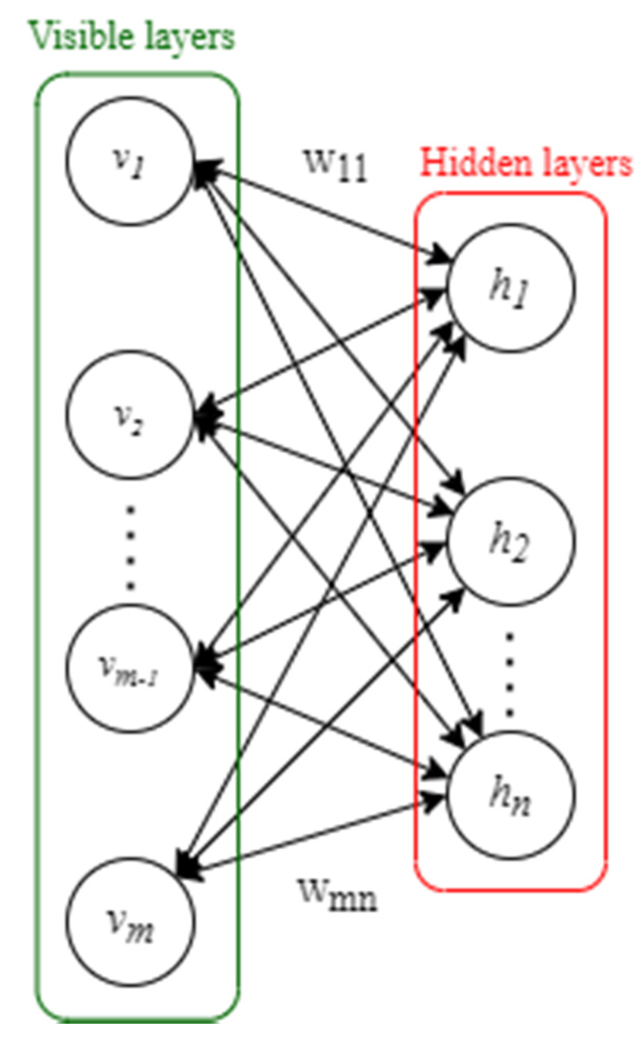
2.1.1. Restricted Boltzmann Machine (RBM)

A restricted Boltzmann machine (RBM) signifies a recurrent neural network with two layers and which forms the foundation of DBNs. The RBM is made up of one visible and one hidden layer, each having $m$ visible units $v=v_1, v_2,\dots ,v_m$ and $n$ hidden units $h=h_1,h_2,\dots ,h_n$, (as shown in Figure 1), and both the visible and hidden components are binary variables with states 0 or 1. The internal neurons of the visible layer and the hidden layer have no connection, while the neurons of the visible layer and the hidden layer are linked by the weight $w$.

Moreover, the RBM is a model that is based on the energy function. The system is thought to be more stable if the energy function is lower. The network energy is reduced, and the optimal parameters of the network are found through training. As a result, the RBM energy function is defined as for a particular set of neuron states $\left(v, h\right)$ and can be written as follows:

$$E\left(v,h\right)=-{\displaystyle \sum }_{i=1}^m{a}_i{v}_i-{\displaystyle \sum }_{j=1}^n{b}_j{h}_j-{\displaystyle \sum }_{i=1}^m{\displaystyle \sum }_{j=1}^n{w}_{ij}{v}_i{h}_j$$

(1)

where $v_i$ represents the state of the ith neuron in the visible layer, $h_j$ represents the state of the jth neuron in the hidden layer, $a_i$ represents the bias of the visible layers $v_i$, $b_j$ represents the bias of the hidden layers $h_j$, and $w_{ij}$ represents the weight between the visible element $v_i$ and the hidden element $h_j$. The weight matrix connecting the visible layer and the hidden layer can be represented by $W$ of size $m\times n$.

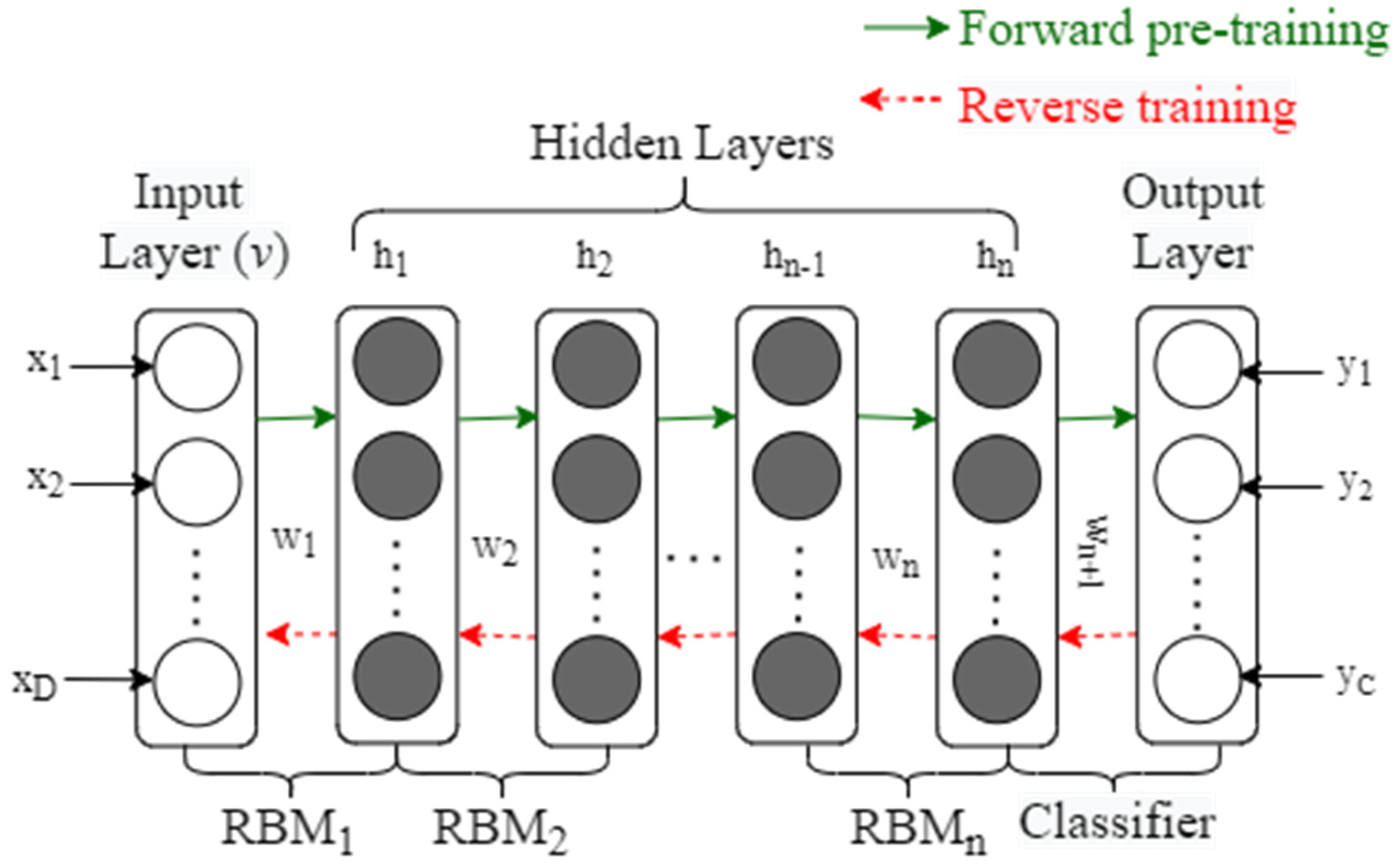
2.1.2. Structure of Deep Belief Network

Figure 2 shows a DBN model stacked by $n$ RBMs and a classifier. ${\mathrm{RBM}}_1$ is composed of the visible layer $v$ (the input layer) and the hidden layer $h_1$, and ${\mathrm{RBM}}_2$ is composed of the hidden layer $h_1$ of ${\mathrm{RBM}}_1$ and the second hidden layer $h_2$ (the output of ${\mathrm{RBM}}_1$ is used as the input of ${\mathrm{RBM}}_2$), and so on, while the hidden layer $h_{n-1}$ of ${\mathrm{RBM}}_{\mathrm{n}-1}$ and the nth hidden layer $h_n$ constitute ${\mathrm{RBM}}_{\mathrm{n}}$, and the output layer is composed of the classifier. The bottom visible layer provides sample features, which are extracted by the middle $n$ layers, and then the classification and recognition results are produced by the top output layer. The input layer contains D units, which correspond to the D-dimensional characteristics of the sample, while the output layer has c units, which correspond to the sample’s c categories, and Weights, $W=\left\{W_1, W_2,\dots , W_{n+1}\right\}$ is the difference between two consecutive layers. The first step is pre-training, utilizing bottom-up training layer-by-layer; then, train RBM₁, and then update the parameters in RBM₁ using forward propagation and reverse reconstruction. RBM₁ training is finished when the maximum number of cycles is achieved. Then, the parameters of ${\mathrm{RBM}}_1$ are fixed and the ${\mathrm{RBM}}_1$ output is used as the input of ${\mathrm{RBM}}_2$ so to train ${\mathrm{RBM}}_2$, and so on, while training $n$ RBMs in turn and obtaining the input layer bias a, the hidden layer bias b, and the weight W between any two adjacent layers corresponding to $n$ RBMs. The original features of the lower layers are merged after layer-by-layer training so to produce a more in-depth and abstract high-level feature extraction. This training approach is also known as unsupervised greedy layer-wise pre-training [11] since the pre-training stage does not need categorized information. The number of hidden layers and units per layer must be determined based on experience.

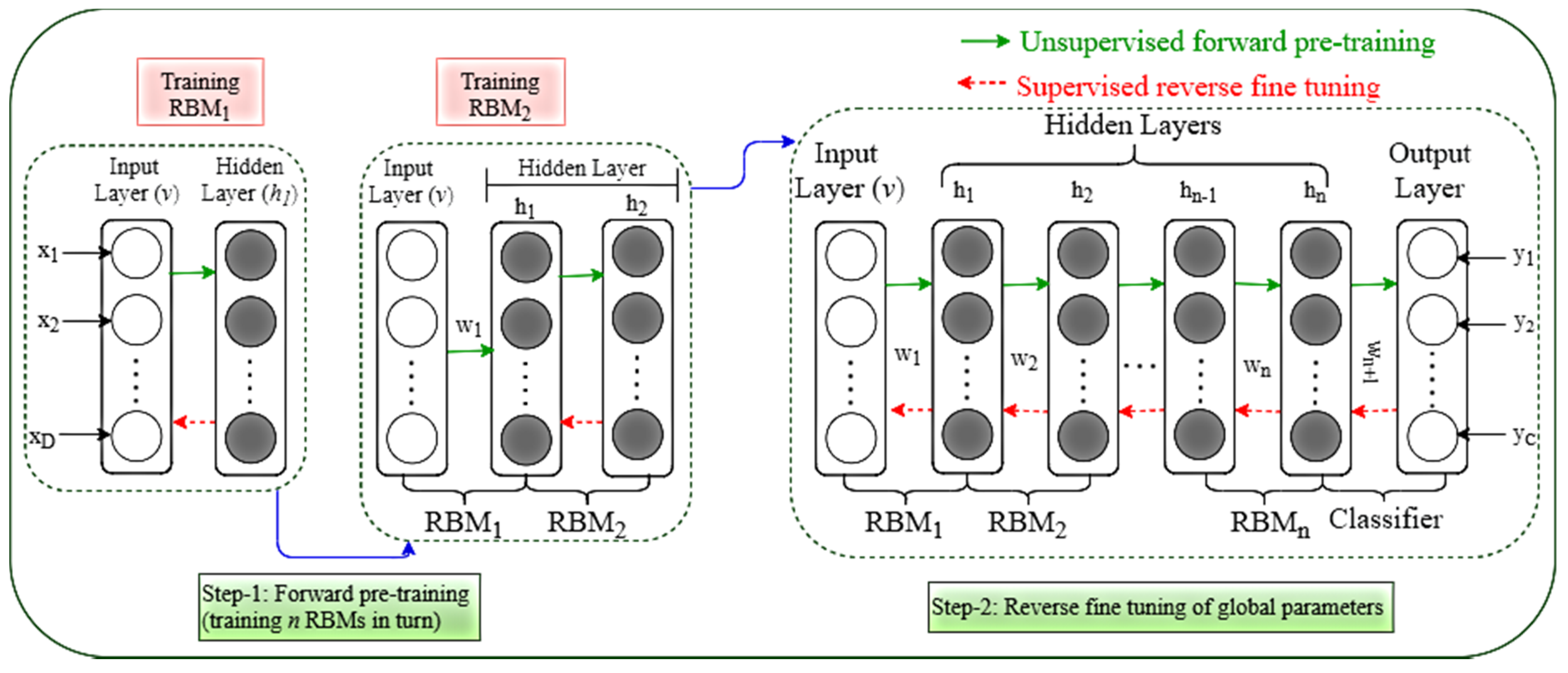
2.1.3. Training of Deep Belief Network (DBN)

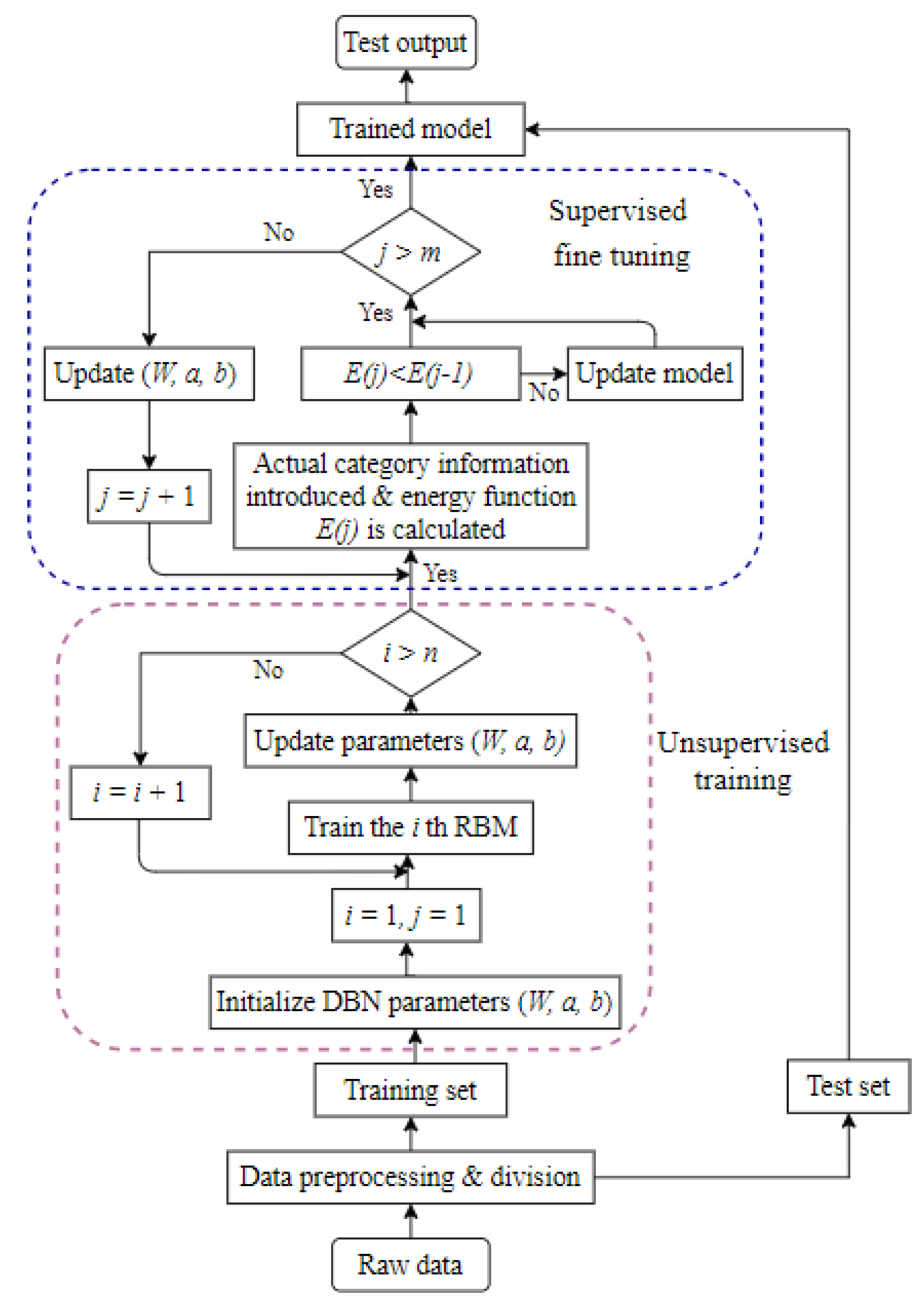
A training flowchart has been presented in Figure 3. Pre-training and reverse fine-tuning are the two steps of the DBN training [20,21]. As this pre-training technique cannot optimize all of the network parameters, the second stage must be used to optimize the global parameters. The fine-tuning stage is the next step. The parameters are changed from top to bottom in the appropriate classifier via backpropagation, culminating in the fine-tuned parameters $\left\{W^{\prime },a^{\prime },b^{\prime }\right\}$. As this stage involves supervised training, since the fine-tuning quantity must be gained by learning categorized information, the fine-tuning procedure is also referred to as supervised fine-tuning. Traditional neural network training methods are not suited for multilayer networks [22], but the DBN semisupervised training method successfully overcomes this problem.

2.2. Self-Encoding Network

A common three-layer unsupervised feature learning model is the autoencoder (AE). The output can be restored to the input as closely as feasible using adaptive learning features [33,34,35]. The corresponding autoencoding network model has evolved according to different standards for defining feature expression, such as sparsity features, noise reduction features, regular constraint features, and so on. Among them, the sparse autoencoding network (sparse AE) and the noise reduction autoencoding network (denoising AE) [40,43,44,45,46,47] are the most commonly used. The multilayer structure of the deep self-encoding network is produced by stacking numerous self-encoding networks, the most widely utilized of which is stacked AE [39,40,41,46,47,48,49,50,51,52]. The original autoencoding network, sparse autoencoding network, denoising autoencoding network, and stacked autoencoding network will all be covered in this section.

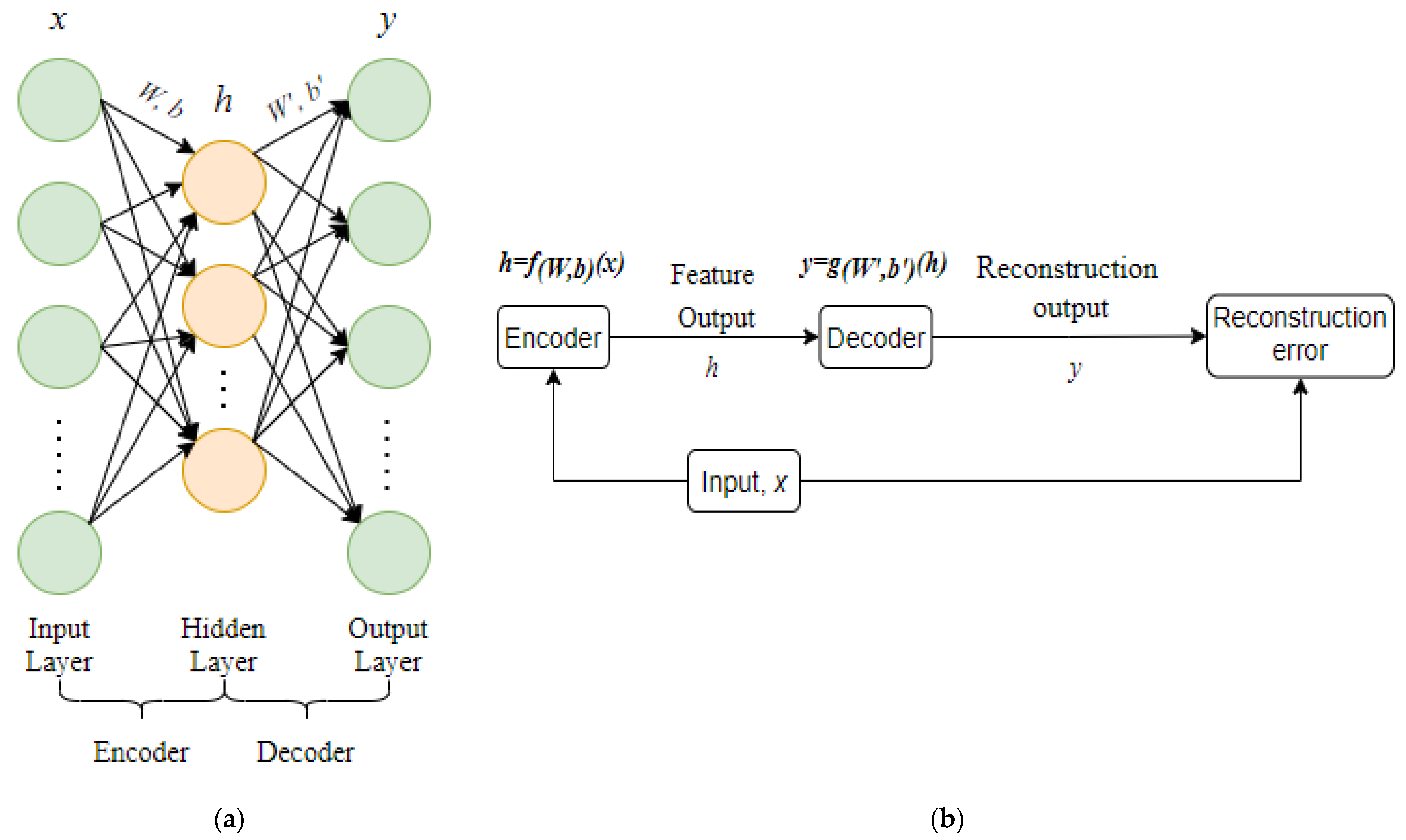
2.2.1. The Original Self-Encoding Network

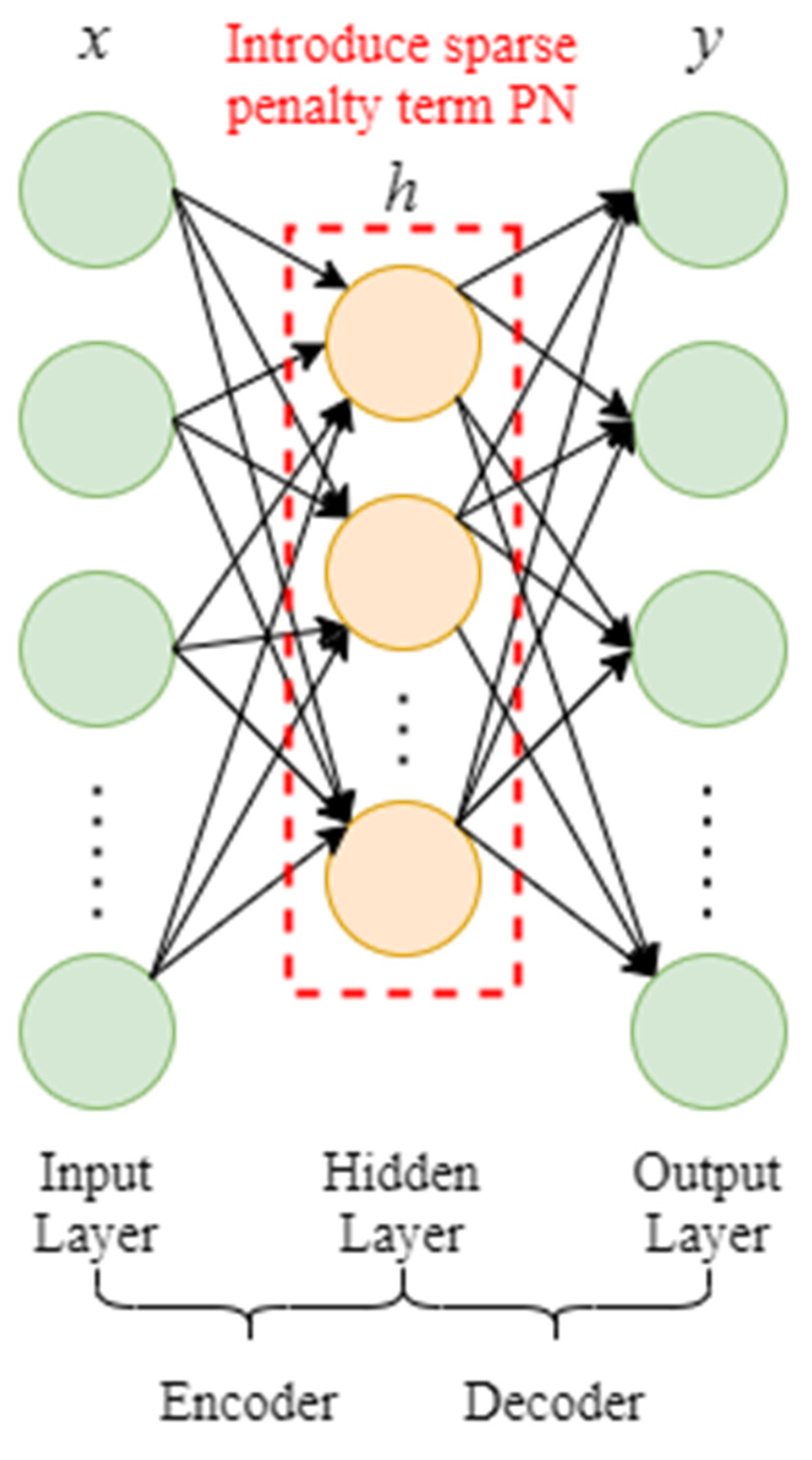
The topological structural diagram of the self-encoding network is shown in Figure 4a. The self-encoding network is a three-layer neural network with an input layer, a hidden layer, and an output layer, as illustrated in Figure 4. It consists mostly of an encoder and a decoder. The encoder is made up of the input layer and the hidden layer, while the decoder is made up of the hidden layer and the output layer. The encoder encodes the original data, the hidden layer obtains the feature output vector, and the feature output vector is subsequently rebuilt into the original data by the decoder. The feature output of the hidden layer is regarded to be the typical expression of raw data when the error between the output data and the input data is minimal enough.

A schematic diagram of the self-encoding network is shown in Figure 4b. Encoding is defined as the process of passing an input $x$ through an encoder to produce a characteristic output $h$, where $h=f_{\left(W,b\right)}\left(x\right)={\mathrm{s}}_f \left(WX+b\right)$, $W$ is the weight matrix connecting the input layer and the hidden layer, $b$ is the bias matrix between the input layer and the hidden layer, and $s_f$ is the activation function of the encoder. Decoding is the process of using the feature output $h$ to reconstruct output $y$ using the decoder, with $y=g_{\left(W^{\prime },b^{\prime }\right)}\left(h\right)=S_g\left(W^{\prime }h+b^{\prime }\right)$, where $W^{\prime }$ is the weight matrix connecting the hidden layer and the output layer, $b\prime$ is the bias matrix of the hidden layer and the output layer, and $s_g$ is the activation function of the decoder. The self-encoding network looks for the best parameters {$W$, $W^{\prime }$, $b$, $b^{\prime }$} to get the reconstructed output $y$ as near as possible to the original signal $x$. Reconstruction error is a measure of how near the input and output are. There are two approaches to characterize reconstruction error, the mean square error and cross-entropy, depending on the type of data:

$$L_{mse}\left(x,y\right)=\frac{1}{m}{\displaystyle \sum }_{i=1}^m\frac{1}{2}{\Vert x-y\Vert }^2$$

(2)

$$L_{ce}\left(x,y\right)=\frac{1}{m}{\displaystyle \sum }_{i=1}^m\left[y\log \left(x\right)+\left(1-y\right)\log \left(1-x\right)\right]$$

(3)

The cross-entropy function can converge quicker since its derivative is steeper, but it is only suited for situations where the value range is between [0, 1]. Due to this property of cross-entropy, the mean square error is utilized when the network output layer employs a nonlinear activation function, whereas cross-entropy is employed when the network output layer employs a linear activation function. The cost function of the self-encoding network can generally be written as,

$$J\left(W,b\right)=L\left(x,g\left(f\left(x\right)\right)\right)+\lambda \times {\mathsf{\Omega }}_{weight}=L\left(x,y\right)+\frac{\lambda }{2}{\displaystyle \sum }_{l=1}^{n_l-1}{\displaystyle \sum }_{i=1}^{S_l}{\displaystyle \sum }_{j=1}^{S_{l+1}}{\left(W_{ij}\left(l\right)\right)}^2$$

(4)

where $L\left(x,y\right)$ is the reconstruction error; $\lambda \mathsf{\Omega }$ is the weight attenuation term to prevent overfitting [35]; $m$, $n_l$, and $S_l$ represent the number of samples, the number of network layers, and the number of neurons in the $l$ layer, respectively; $W_{ij}$ represents the weight of the interlayer connection; $b$ is the unit bias of the $l$ layer.

2.2.2. Sparse Autoencoding Network

The sparse autoencoding network (sparse AE) is based on the sparse coding principle. The sparse penalty term is added on the basis of the autoencoding network model, that is, the hidden layer meets the sparsity so that the autoencoding network may learn to express relatively sparse and compact feature expressions within the sparsity restriction [36,37,38,39,40,41,42]. The activation state (active) for neurons in the hidden layer is defined as when its value is near to 1 and close to 0 (corresponding to the sigmoid activation function) or −1 (corresponding to the $tanh$ activation function) (not activated). Sparse restriction occurs when the restricted neurons are blocked in most states and activated in a few others. Figure 5 represents the layout of the sparse autoencoding network.

Under normal conditions, the sparse penalty term PN is chosen as the Kullback–Leibler (KL) divergence, as shown in Equation (5):

$$PN={\displaystyle \sum }_{j=1}^{S}KL(\rho ||\widehat{{\rho }_j})={\displaystyle \sum }_{j=1}^s\rho \ln \frac{\rho }{\widehat{{\rho }_j}}+\left(1-\rho \right)\ln \frac{1-\rho }{1-\widehat{{\rho }_j}}$$

(5)

where $S$ is the number of units in the hidden layer, $\rho$ is a sparse constant close to 0, and $\widehat{{\rho }_j}$ is the average activation of the $j\mathrm{th}$ unit. When $\widehat{{\rho }_j}=\rho$, the KL divergence value is 0, and the KL divergence value gradually increases as $\widehat{{\rho }_j}$ deviates from $\rho$. Then refer to formula (4), the autoencoding network containing the sparse penalty term and the cost function can be written as,

$$J_{sparse}=J\left(W,b\right)+\beta \times PN$$

(6)

where $\beta$ is the coefficient of the sparse penalty term.

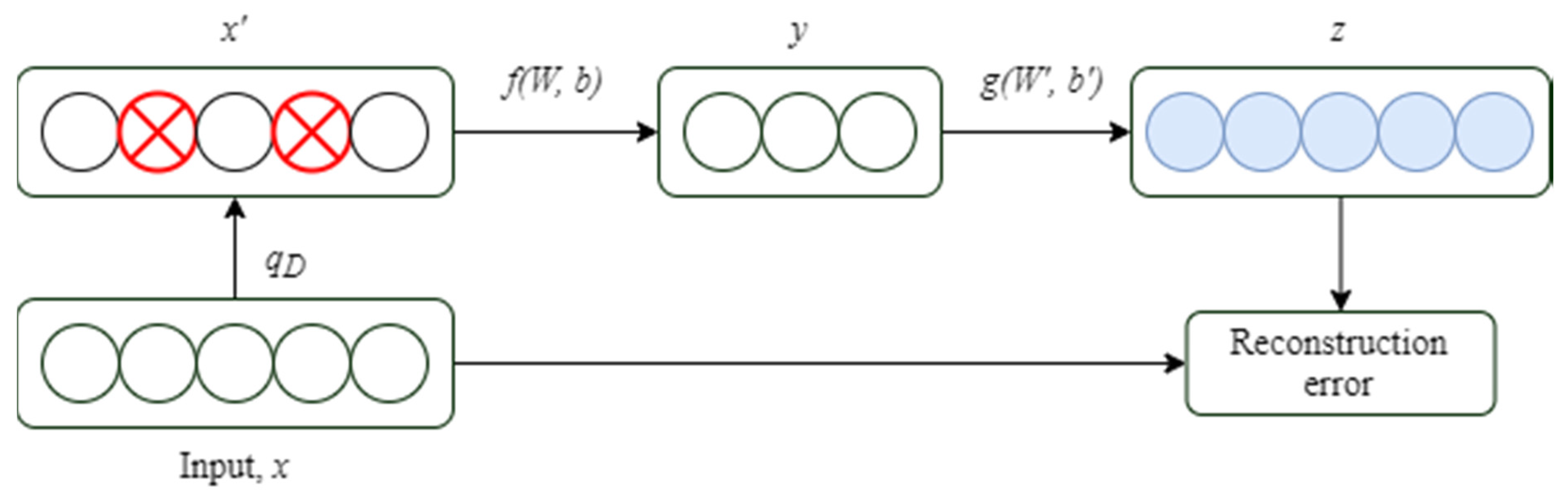
2.2.3. Noise Reduction Self-Encoding Network

Pascal Vincent et al. [43] proposed the denoising AE (DAE). After encoding and decoding the original sample signal, noise with specific statistical characteristics was randomly added and the final mapping returned an undisturbed noise which is the sample signal that was affected. The idea behind the denoising self-encoding network is similar to that of the human body’s sensory system. For instance, when the human eye examines an object, even if a tiny portion is obscured the human may still recognize the object. Similarly, the noise reduction self-encoding network accomplishes decoder reconstruction by introducing noise, thereby effectively minimizing the impact of random variables on signal extraction such as mechanical working conditions or ambient noise. The denoising self-encoding network has considerably enhanced generalization and feature expression abilities, as well as resilience, when compared to the original self-encoding network [43,44,45,46,47].

Figure 6 shows the construction of the noise reduction self-encoding network, which uses a random mapping $x^{\prime }~q_D(x^{\prime }|x)$ [43] to interfere with the original signal x to mimic noise and produce the signal $x\prime$. To retrieve the feature output, encode $x\prime$ through the encoder: $y=f_{\left(W,b\right)}\left(x^{\prime }\right)=S_f\left(W{x}^{\prime }+b\right)$, where $W$ is the weight matrix linking the input layer and the hidden layer, $b$ is the bias matrix between the input layer and the hidden layer, and $s_f$ is the encoder’s activation function. After decoding the feature expression $y$ through the decoder, a reconstructed and pollution-free signal is obtained, $z=g_{\left(W^{\prime },b^{\prime }\right)}\left(y\right)=s_g\left(W^{\prime }y+b^{\prime }\right)$, where $W^{\prime }$ is the weight matrix connecting the hidden layer and the output layer, $b^{\prime }$ is the bias matrix in between the hidden layer and the output layer, and $s_g$ is the activation function of the decoder. By seeking the optimal parameters {$W, W^{\prime }, b, b^{\prime }\},$ the reconstructed output $z$ is as close as possible to the original signal $x$. The reconstruction error of the denoising autoencoding network still indicates the closeness of the input and output when compared to the original autoencoding network, but the characteristic output $y$ of the denoising autoencoding network is obtained by mapping the signal $x\prime$ which is affected by the noise instead of the original signal $x$, thereby forcing the denoising self-encoding network to learn a more intelligent mapping, which is a feature extraction method that is conducive to denoising.

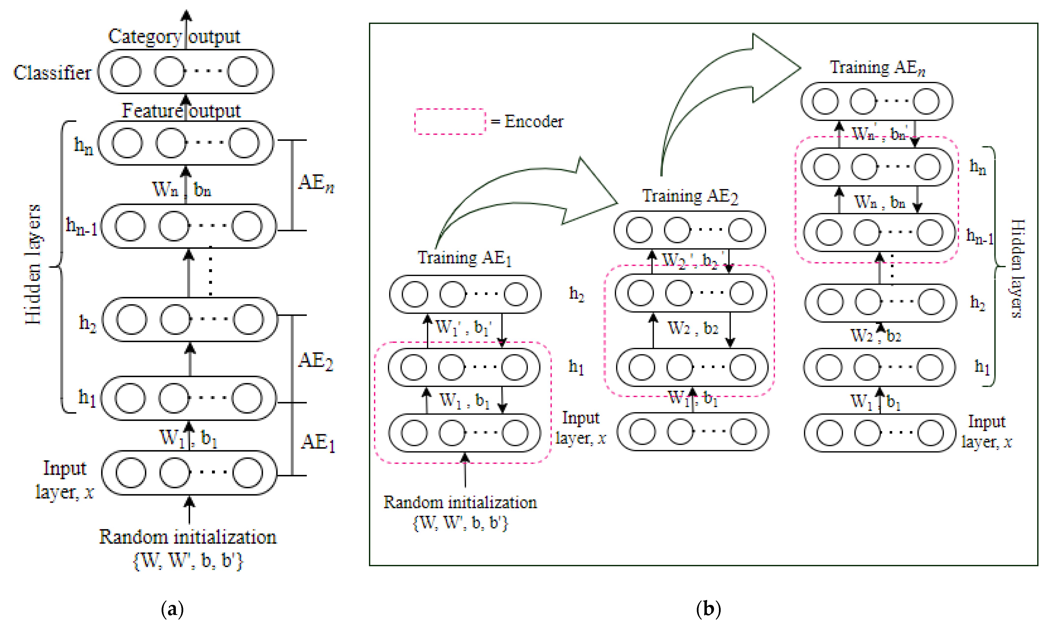
2.2.4. Stacked Self-Encoding Network

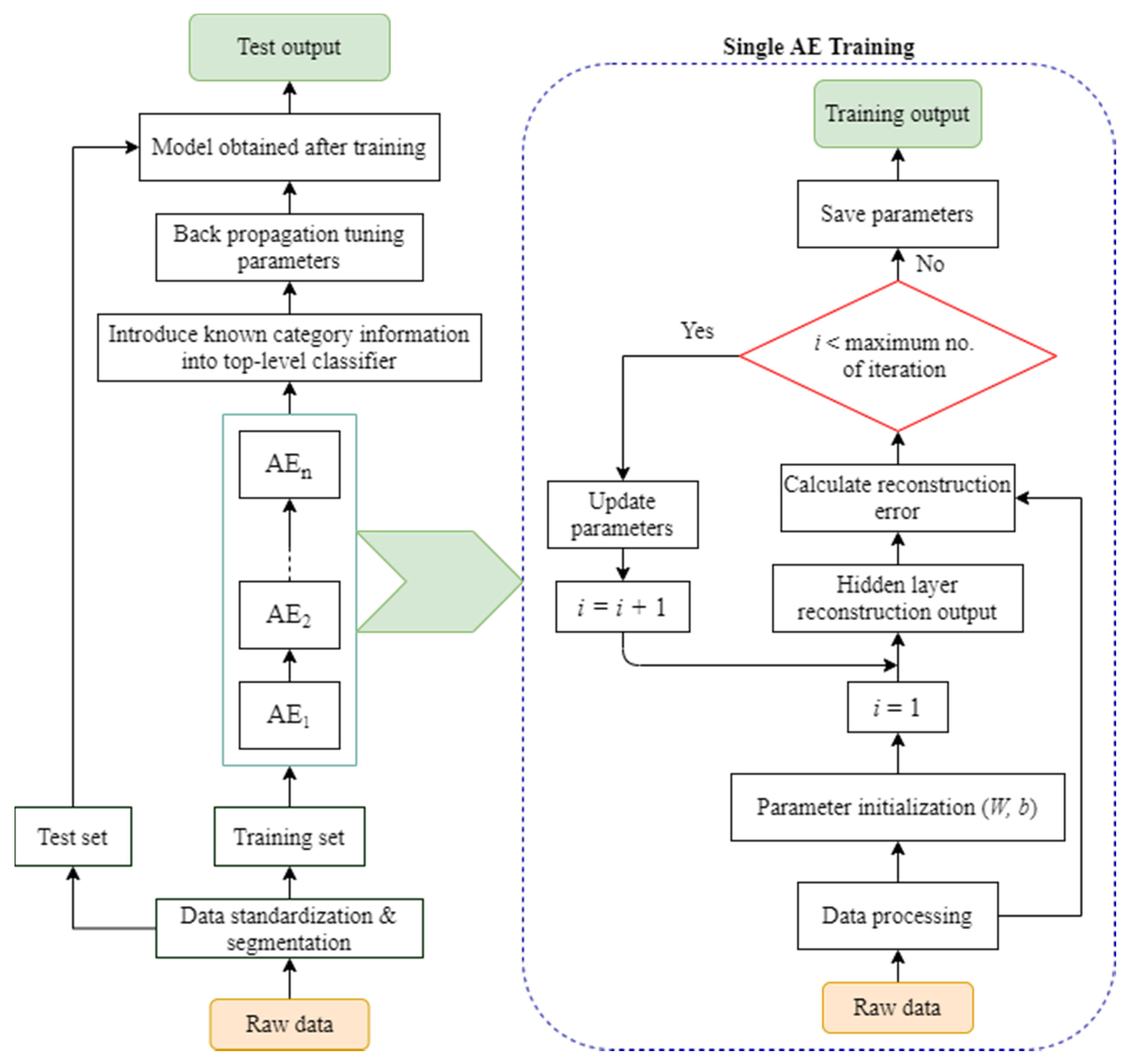
An autoencoding network (AE) is the basic unit of a stacked autoencoding network (stacked AE), but it can also be a sparse autoencoding network evolved from AE, a noise-reducing autoencoding network, etc. The greedy layer-by-layer training method proposed by Hinton et al. [10] is used in the stacked self-encoding network, which solves the problem that traditional neural network training algorithms tend to fall into local extremes. As shown in Figure 7a, the stacked self-encoding network is formed by stacking multiple self-encoding networks which can learn the characteristics of the original data layer-by-layer. Each layer’s input is based on the previous layer’s feature output. Each layer feature expression is more abstract than the one before it. A classification layer is frequently placed at the top of the stacked self-encoding network for the classification tasks. The stacked AE is more appropriate for applications such as complicated categorization than the original autoencoder network.

The stacked AE network’s training method is comparable to that of the DBN, which are separated into two stages: forward training and reverse fine-tuning. The forward training of the stacked self-encoding network is seen in Figure 7b. Train $A{E}_1$, then randomly set the initial weights and biases of $A{E}_1$ $\left\{W, W^{\prime }, b, b^{\prime }\right\}$ according to formula (4), compute the input and output reconstruction errors, then use the backpropagation method to adjust the parameters in $A{E}_1$, and the process continues to update until the reconstruction error is the least. At this point, only the encoder portion of $A{E}_1$ is retained, and the feature output of $A{E}_1$ is used as the input of $A{E}_2$ to train $A{E}_2$, and so on, until all n $AEs$ have been trained. When $AE$ has finished training, the final feature output is the hidden layer output of $AEn$. The reverse fine-tuning stage of the stacked autoencoding network can adjust the parameters of the entire network (this is similar to the DBN and is suitable for large amounts of training data) or it can only adjust the parameters of the classifier. The coding network is known as a feature extractor.

2.3. Convolutional Neural Network (CNN)

A prominent deep learning model is the convolutional neural network (CNN). Local perception, shared weights, and spatial or temporal downsampling are hallmarks of the CNN [53,54,55], which minimizes the parameters and makes maximum use of the data’s local characteristics.

An input layer, several hidden layers, a fully connected layer, and an output layer make up a CNN. A convolutional layer and a sub-sampling layer make up the majority of the hidden layer. Data in the form of images or vectors can be used as input. The convolutional layer is mostly utilized for feature extraction. The sigmoid function is frequently chosen as the activation function of the convolutional layer in classic CNNs. Several convolution kernels make up a convolutional layer. Each convolution kernel can be considered as a filter in its own right. Each filter scans the input picture or the data according to the scanning step length (each filter scans the image or data once local), and each scan is done with the same weight and offset (i.e., different filters use different weights and offsets). After convolution, the vector size is $\left(n-k+m\right)/m$, where $n$ is the input vector size,$k$ is the convolution kernel size, and $m$ is the scan step size. Human experience must be used to control the size and number of convolution kernels, as well as the scanning step length. Here is the mathematical model of the convolution layer,

$${x_j}^l=f\left({\displaystyle \sum }_{i\in M_j}{x_i}^{\left(l-1\right)}\times {K_{ij}}^l+{b_j}^l\right)$$

(7)

where $M_j$ is the input feature; $l$ is the layer $l$ network; $K$ is the convolution kernel; $b$ is the bias; ${x_j}^l$ is the output of the $l$ layer; ${x_i}^{\left(l-1\right)}$ is the input of the $(l-1$) layer, which is also the input of the $l$ layer.

The main purpose of the sub-sampling layer is feature dimensionality reduction, also known as pooling. The sub-sampling procedure can be thought of as dividing the features acquired by convolution into numerous discrete sections and then choosing the maximum value (maximum pooling method) or average value (mean pooling method) of the data in each region as the features after sampling. The degree of feature sparsity is represented by the size of the sub-sampling. The sparsity impact is stronger, and the resulting features are more robust as the size increases. The mathematical model of the sub-sampling layer is,

$${x_j}^l=f\left({{\beta }_j}^{l}down\left({x_i}^{l-1}\right)+{b_j}^l\right)$$

(8)

where down(.) is the sub-sampling function and $\beta$ is the network multiplicative bias.

The CNN is a supervised deep learning algorithm. It uses a similar training strategy to artificial neural networks. It typically employs a backpropagation technique to pass errors layer-by-layer, and a gradient descent to update the network parameters.

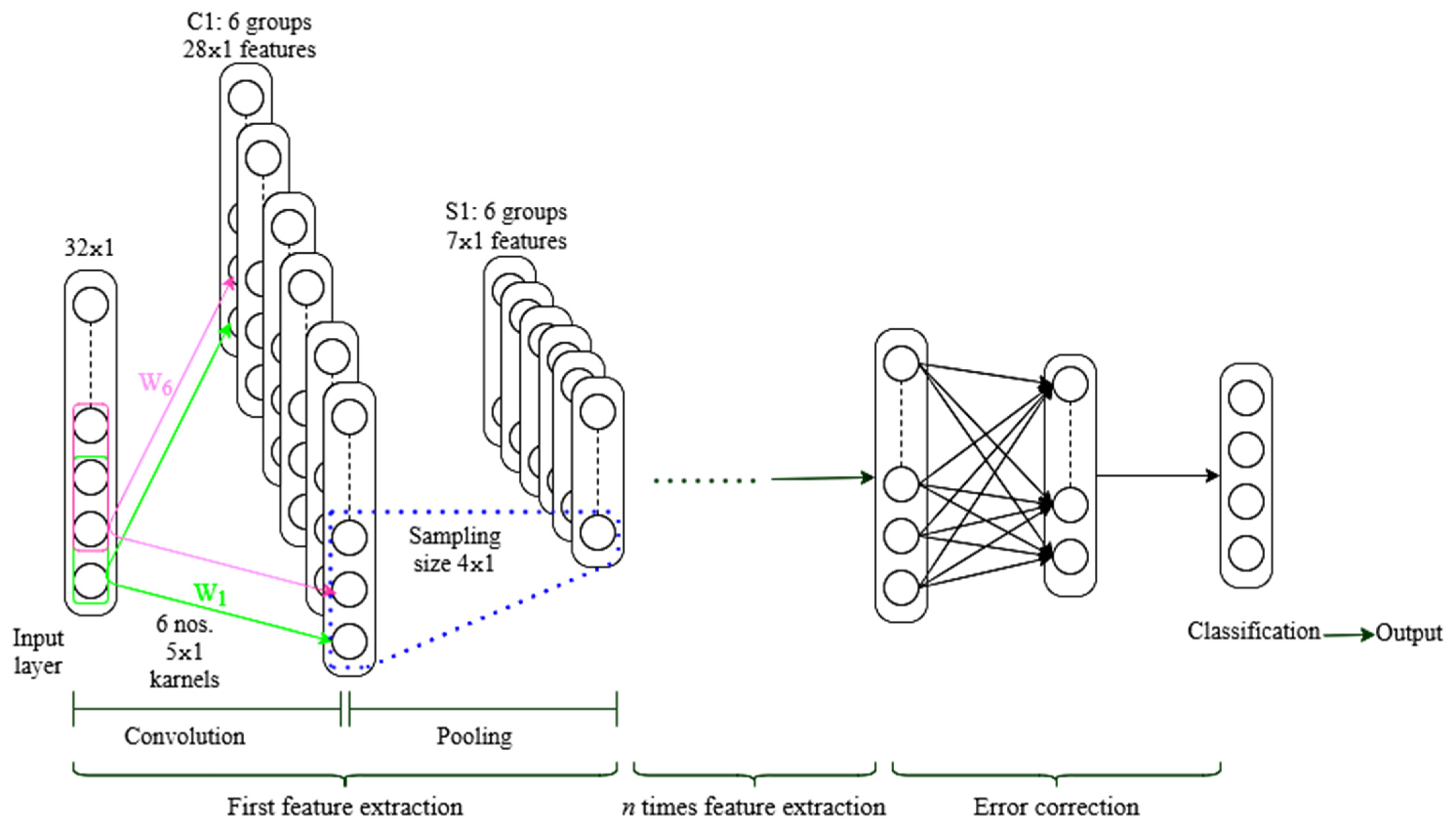
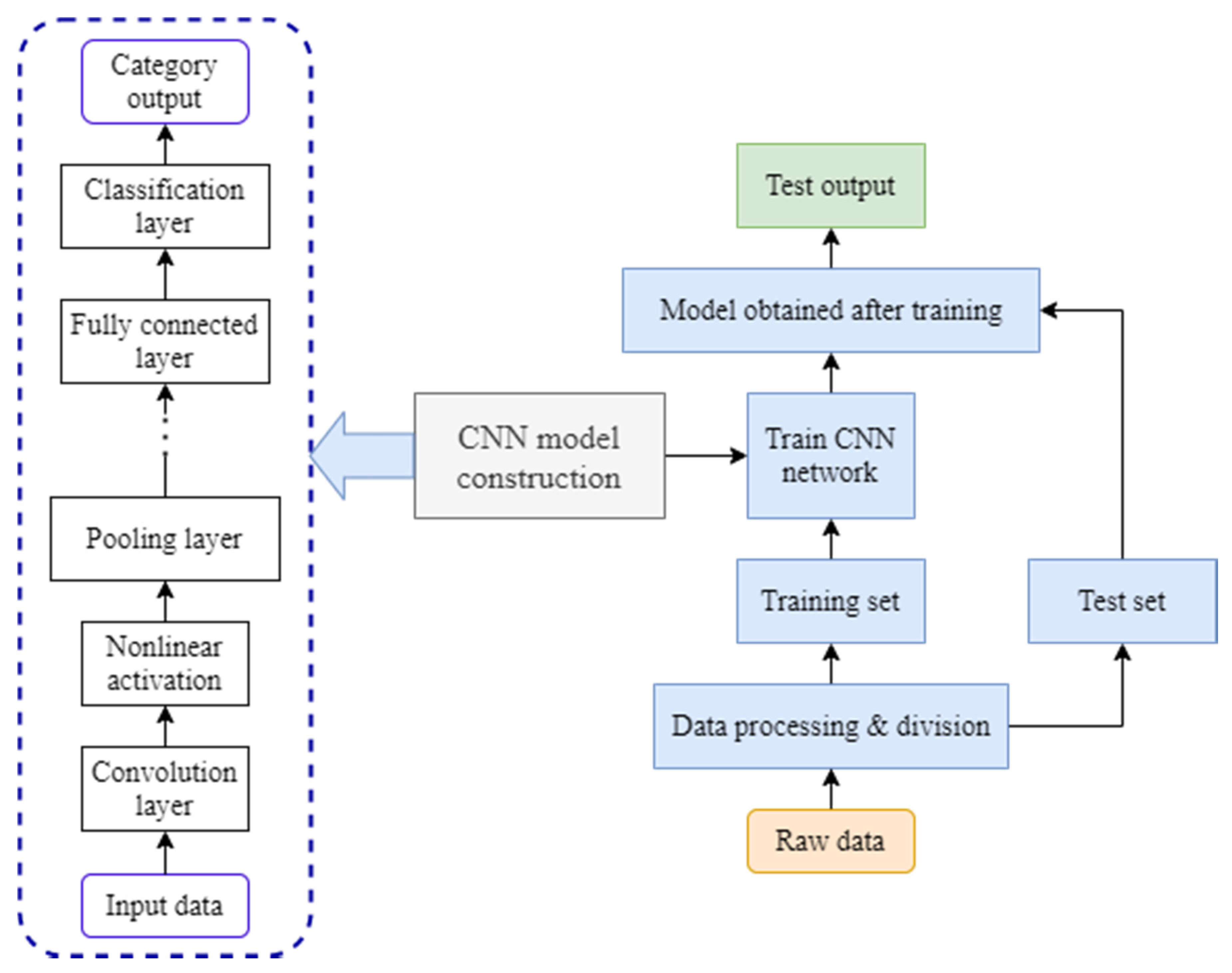
To understand the process, consider time series signal processing, as illustrated in Figure 8. The output is the classification result while the input is a 32 × 1 signal. Select 6 groups of 5 × 1 convolution kernels, and the step size is 1, to generate 6 groups of 28 × 1 features, where 28 = (32 − 5 + 1)/1, and the neurons in C1. Only a few neurons in the previous layer are linked to the cell. The sub-sampling layer is S1. Select 7 × 1 as the sub-sampling size for the maximum pooling approach, then divide the 6 groups of features in C1 into blocks. Each block is 4 × 1 in size, and by taking the maximum value of each block, 6 sets of 7 × 1 features can be obtained. The collected features are processed in the fully connected layer after multiple convolutions and pooling, and the category output is obtained in the output layer. The fully connected layer, for example, employs a common layer or multi-layer neural network [53], in which each neuron in one layer is linked to all neurons in the preceding layer.

2.4. Recurrent Neural Network (RNN)

The DBN, AE, and CNN all presume that elements are independent of one another, as well as input and output. However, many factors are intertwined. The output of a recurrent neural network (RNN) is dependent on the current input and memory, and it connects the units in the same layer to construct a directed cyclic neural network [61]. Hundreds of RNN topologies have been proposed to suit the demands of a wide range of dynamic performance [62]. The Jordan network [62,63,64,65] and the Elman network [62,63,65] are the two of the most well-known RNN models.

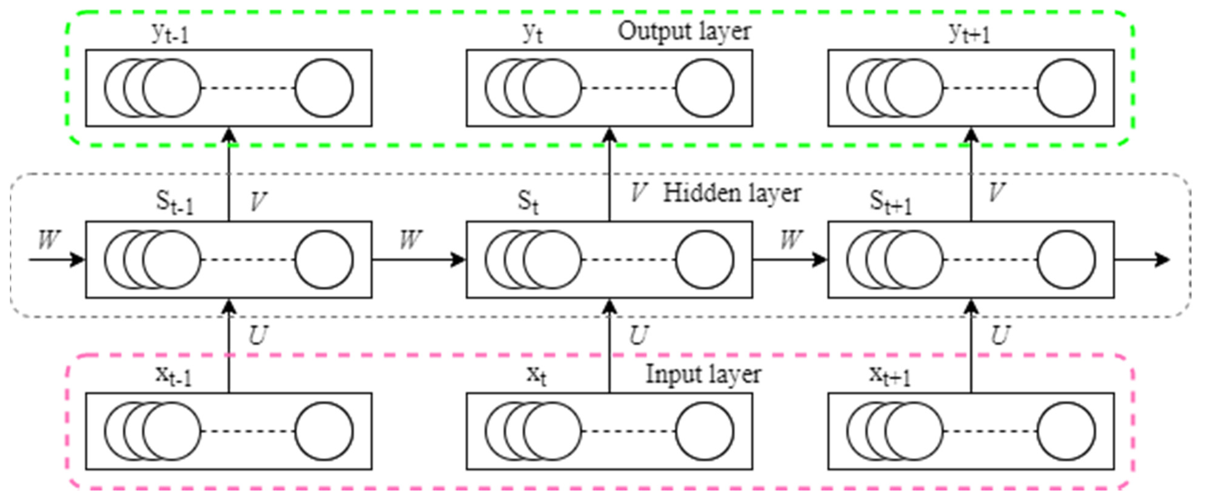
The basic structure of the RNN is depicted schematically in Figure 9. The hidden layer unit not only takes data input at the current time but also receives hidden layer output at the prior time, as shown in the diagram. As a result, the network may recall earlier knowledge. Equation (9) provides the network’s mathematical model.

$$\begin{array}{c}{S}_t=f\left(W{S}_{t-1}+U{x}_t\right)\\ y_t=g\left(VS\right)\end{array}$$

(9)

where $x_{t-1}$, $x_t$, and $x_{t+1}$ correspond to the input at $t-1, t,$ and $t+1,$ respectively; $S_{t-1}, S_t,$ and $S_{t+1}$ correspond to the hidden input at $t-1, t,$ and $t+1$, respectively, and the layer state; $y_{t-1}$, $y_t$, and $y{ }_{t+1}$ correspond to the output at $t-1, t,$ and $t+1$, respectively; $f$ and $g$ are activation functions; $U, W,$ and $V$ correspond to the weight from the input layer to the hidden layer, the weight from the hidden layer to the hidden layer, and the weight from the hidden layer to the output layer, respectively.

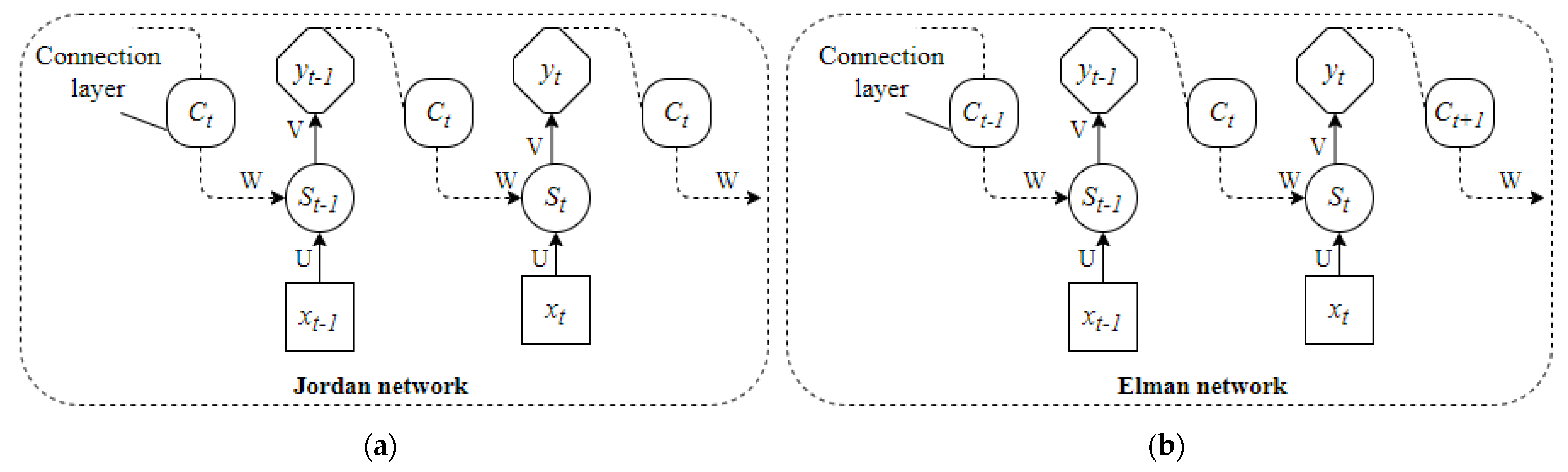
Figure 10 depicts the first and most well-known RNN structures: the Jordan and Elman networks. Figure 10a shows that the Jordan network adds a connection layer to the basic RNN and uses the previous time’s feedback and the current time’s network input as the hidden layer input at the current time, which is comparable to output feedback. The Jordan network’s mathematical model is,

$$\begin{array}{c}{S}_t=f\left(W\times C_t+U\times x_t\right)\\ C_t=y_{t-1}+\alpha C_{t-1}\\ y_t=g\left(V\times S_t\right)\end{array}$$

(10)

where $x_t$ is the input at time t; $S_t$ is the hidden layer state at time t, and $y_{t-1}$ is the output at time $t-1$; $C_{t-1}$ and $C_t$ are the output of the connection layer at time $t-1$ and $t$, respectively; $\alpha$ is feedback gain factor;$f$ and $g$ are activation functions; $U, W,$ and $V$, respectively, correspond to the weight from the input layer to the hidden layer, the weight from the connection layer to the hidden layer, and the weight from the hidden layer to the output layer.

By linking the layers, the Elman network uses the hidden layer state at the previous instant and the network input at the present moment as the hidden layer input at the present moment, which is similar to state feedback, as shown in Figure 10b. The Elman network’s mathematical model is,

$$\begin{array}{c}{S}_t=f\left(W\times C_t+U\times x_t\right)\\ C_t=S_{t-1}+\alpha C_{t-1}\\ y_t=g\left(V\times S_t\right)\end{array}$$

(11)

The Jordan network can only convey the output properties, whereas the Elman network incorporates state feedback. In comparison, the Elman network is superior at expressing dynamic systems [61,63].

3. Application of Deep Learning in Electric Motor’s Fault Diagnosis

Bearing faults, stator faults, rotor faults, and air gap eccentricity faults are all common motor defects, with bearing failures having the highest probability and rolling bearings being prone to gearbox faults.

Signal processing approaches combined with classification algorithms (such as support vector machines, decision trees, K closest neighbors, etc.) are frequently used in classical fault detection to categorize and identify defects. The signal processing method is one of them, and it employs several approaches depending on the type of fault. When a motor bearing fails, for example, vibration signals or stator current signals are frequently used, and time–frequency domain analysis, statistical analysis, wavelet decomposition, and other methods are used to extract features from the signal when the motor rotor fails, while the time–frequency domain analysis, statistical analysis, wavelet decomposition, and other methods are used to extract features from the signal. The stator current detection method is the most often utilized. The features of the stator current signal are retrieved using the Fourier transform or the Hilbert transform since the stator current signal is straightforward to gather. When a motor stator breaks, a mathematical model or the determination of the motor problem is typically applied. The defect is diagnosed using the current and voltage signal detecting approach. When using the signal detection method, feature extraction calculations are still required; however, when the motor has an air gap eccentric defect, the current signal analysis approach is frequently utilized to diagnose the fault.

Artificial feature selection and extraction are always necessary for the generally used traditional motor fault diagnosis methods, which raises the uncertainty of the motor fault diagnosis and affects the accuracy of motor problem diagnosis. The deep learning model may extract features from the source signal in an adaptive manner, thereby avoiding the impact of artificial feature extraction.

3.1. Application of Deep Belief Network (DBN)

Since the DBN was introduced in 2006, it has been employed mostly in the field of machine vision. The DBN was initially used in the field of fault diagnosis in 2013. A DBN-based aircraft engine failure diagnosis approach was proposed by Tamilselvan et al. [18]. Although the DBN is used as a classifier in this method to achieve fault classification, the DBN-based feature extraction is not implemented. However, it has aided in the development of a DBN-based fault diagnosis approach. Tran et al. [19] introduced the DBN to compressor failure diagnosis in 2014, thereby promoting the DBN’s growth in the fault diagnostic sector. Xie et al. [23] have established a DBN model based on Nesterov momentum optimization that captures the frequency domain signals from rotating machinery, feeds them into the model for feature learning and classification, and achieves simultaneous bearing fault category and fault level diagnosis. The author also employed the traditional DBN model and support vector machine (SVM) to classify the same signal and used trials to show that the optimized DBN model has the highest classification accuracy among the three approaches $(\mathrm{optimized} \mathrm{DBN} \mathrm{model} > \mathrm{traditional} \mathrm{DBN} > \mathrm{support} \mathrm{vector} \mathrm{machine})$. During the simulation phase, Li Mengshi et al. [27] proposed a DBN-based fault diagnostic technique for wind turbines, which built a fault diagnosis model using a DBN network and employed Gaussian noise to simulate the noise in the actual operational environment of the wind turbine. Sensor faults, actuator faults, and system faults are among the nine categories of faults. Simultaneously, the author compared the DBN model to Bayesian classification, the random forest classification, the K-nearest neighbor algorithm, and decision trees, the four standard diagnostic approaches, and utilized tests to show that the DBN-based diagnosis method was more robust and stable.

The DBN has been widely employed in the field of motor defect diagnosis, including in rolling bearings [23,24,25,26], wind turbines [27,28], sensors [9,29], gearboxes [30,31,32], and so on, in just a few years of development, and feature extraction based on the DBN has been realized.

Figure 11 depicts a fault diagnostic framework based on the existing DBN-based motor fault diagnosis method, which consists mostly of the following steps:

Step—1:

Obtain the time/frequency domain signals of the equipment under normal and fault situations using sensors and signal preprocessing technologies;

Step—2:

Split the signal into training and test sets after segmenting and normalizing it;

Step—3:

Create a multi-hidden-layer DBN model and utilize the training data for layer-by-layer unsupervised and greedy training;

Step—4:

Use category information to fine-tune the DBN model parameters;

Step—5:

Perform fault diagnosis on the test set using the trained DBN model.

3.2. Application of Self-Encoding Network

Shallow networks include the original autoencoding network, as well as its evolved sparse autoencoding network and denoising autoencoding network. They are frequently piled into deep-stacked autoencoding networks in practical applications. Due to their strength, stacked autoencoding networks are popular. The ability to understand data properties is something that many experts and academics pay attention to. A deep sparse self-encoding network is used in the literature [42] to detect a permanent magnet synchronous motor’s turn-to-turn short-circuit defect. Negative sequence current and torque signals make up the sample. To increase the sample size and create a training set, the generative confrontation network (GAN) is utilized. For classification testing, the sparse self-encoding network created via sample training is used, and the experiment shows that it has a classification accuracy of 99.4%. The literature [46] proposed a multilayer denoising autoencoder network (SMLDAEs) for wind turbine gearbox fault diagnosis because the vibration signal comprises a lot of noise and most denoising autoencoding networks utilize a single noise to train the network. This strategy trains the network with varying noise levels, allowing it to learn more detailed and general fault characteristics from the vibration signal. This classification method is accurate after the experimental verification. The accuracy rate has been consistent in the range of 97.5 to 98 %. To diagnose rolling bearing faults, the literature [39] employs a deep autoencoding network. To improve the denoising ability, minimize computational complexity, and the training convergence speed, they integrate a sparse autoencoding network with a noise-reducing autoencoding network. This method is more robust and can increase the accuracy of rolling bearing failure diagnosis more efficiently. A defect diagnosis approach for rolling bearings and planetary gearboxes based on a stacking autoencoding network was proposed in the literature [41]. This study uses stacking autoencoding networks to classify ten different types of bearing and gearbox problems under various loads. The accuracy percentage for the classification is 99.68%. It shows that the method has a greater diagnostic accuracy than the shallow neural network fault diagnosis method. Since its inception, the stacked autoencoding networks have been applied to rotating machinery [39,45], wind turbines [46,48], rolling bearings [40,49,50], gears [51,52], and aviation equipment, among other fields, with promising outcomes. Furthermore, the literature [33] has elaborated on the self-encoding network development process, detailed the principles of more than ten different types of self-encoding networks, and has conducted a comparison study.

The diagnosis framework is depicted in Figure 12 and summarizes the available electric motor fault diagnosis approaches based on deep self-encoding networks. It essentially contains the following steps:

Step—1:

Obtain signals from the equipment in both normal and defective states using sensors;

Step—2:

Separate the signal into training and test sets by preprocessing it;

Step—3:

Create a deep self-encoding network model based on the data selection reconstruction error and use the training set for unsupervised and greedy layer-by-layer training;

Step—4:

Add a classification algorithm to the top layer, then tweak the parameters of the entire deep self-encoding network or simply the classifier parameters as needed;

Step—5:

Perform the defect diagnosis on the test set using the learned deep self-encoding network model.

Self-encoding networks, also known as deep self-encoding networks, are primarily utilized for noise reduction and feature extraction in the context of fault detection. In comparison to DBN, the self-encoding network training involves fewer samples, and the feature extraction has a higher ability while being more robust.

3.3. Application of Convolutional Neural Network (CNN)

The CNN has local perception and weight sharing properties, reducing the number of network parameters and preventing network overfitting to some level. As a result, it has attracted the attention and research of numerous researchers. As the activation function in traditional CNN is often a saturated nonlinear function such as the sigmoid function or the $tanh$ function, the literature [56,57] suggested and shown that an unsaturated nonlinear function (ReLU function) can improve the CNN network performance. A method based on the CNN gearbox vibration signal fault diagnosis approach was proposed in the literature [58], but the method still requires manually extracting features to construct the input. The literature [59] has developed a CNN-based gearbox vibration signal fault diagnosis approach that can adaptively learn features in response to this challenge. The literature [72] has also presented a new multiscale convolutional neural network (MSCNN) architecture for simultaneous multiscale feature extraction and classification so to address the problem of intrinsic multiscale characteristics in gearbox vibration signals. This strategy employs a number of different techniques. The convolutional layer and the subsampling layer have a hierarchical learning structure that increases the feature extraction efficiency and the diagnostic performance. A diagnostic framework (DTS-CNN) based on the features of motor vibration signals was developed in the literature [73]. This method adds misalignment before the convolutional layer of the CNN rather than using the recovered original vibration signals as the input. The layer extracts the relationship between signals at different intervals in a periodic mechanical signal, overcomes the limitations of standard neural networks, and is more suitable for modern induction motors, especially in nonstationary settings. A real-time motor failure detection approach based on the one-dimensional CNN was proposed in the literature [74]. In the training phase, this method extracts high-resolution features using a large number of one-dimensional filter kernels and then combines the classification algorithms so to extract the characteristics of real-time motor current inputs, and the classification achieved an accuracy rate of higher than 97%. In the literature [75], an intelligent composite fault diagnosis method based on deep decoupling CNN is proposed which addresses the limitations of the traditional fault diagnosis methods in compound fault diagnosis (e.g., a lack of consideration of the connection between a single fault and a compound fault, whereas traditional classifiers can only output one label for the detection samples of compound faults, etc.). The limitation of the fault diagnosis method allows for the reliable identification and decoupling of compound faults. The approaches of the CNN used in the field of electric motor fault diagnosis can be effectively split into two types based on the existing literature. One method is to employ the CNN as a classifier [58,60,75]. Data preparation and feature extraction are required at this time. The other option is to utilize the CNN as a feature extraction and recognition classification model [59,72,73,74,75] and classify while applying adaptive feature learning.

Figure 13 depicts the CNN-based motor defect diagnosis system. The following are the main steps in order:

Step—1:

Obtain the time domain or frequency domain signals from the equipment under normal and abnormal conditions using sensors;

Step—2:

Separate the signal into training and test sets by preprocessing it;

Step—3:

Using the received data, determine the size, number, scanning step, and the number of hidden layers of the CNN and create a CNN model;

Step—4:

Use the training set for supervised training after initializing the CNN network parameters and keep updating the network parameters until the maximum number of iterations is reached;

Step—5:

Perform the fault diagnostics on the test set using the trained CNN model.

The CNN is a deep learning model that specializes in processing large amounts of data, but it has limits when it comes to diagnosing electric motor faults. The CNN is often limited to processing one-dimensional signal data, with the multidimensional data processing capabilities being limited. In terms of the types of faults the CNN for multidimensional data processing can handle, more research is needed [61].

3.4. Application of Recurrent Neural Network (RNN)

The RNN is a neural network model that excels in processing time series and boasts fast convergence, high accuracy, and high stability. In terms of defect diagnosis, the RNN is particularly well suited to complicated equipment or systems [68,69,70,71].

According to the literature [76], the typical RNN has the problem of gradient disappearance or gradient explosion, which prevents it from using information from the past; therefore, a long- and short-term memory neural network (LSTM) is proposed to tackle this problem as it addresses the gradient problem and has benefits in processing data with a strong correlation with time series. The LSTM is widely employed in the field of fault diagnostics [77,78,79,80,81]. An electric motor defect detection approach based on the LSTM was proposed in the literature [78]. The real-time prediction of the three-phase current value of the next sample instant was utilized to observe the motor in real-time by capturing the three-phase current value and phase angle information of the previous sampling data. In the literature [79], the feature vector of the vibration signal of the rolling bearing of a wind turbine is extracted using a wavelet packet transform, and the LSTM is used as a classifier to diagnose three frequent problems of the rolling bearing of a wind turbine. Through a case study, the literature verifies the usefulness of the method. It demonstrates that LSTM can still perform well in fault diagnosis when the difference in the fault feature quantity is not significant. The literature [80] utilized empirical mode decomposition and LSTM to provide rotating machinery state monitoring and prediction. When compared to support vector regression machine (SVRM), it was found that LSTM can effectively avoid parameter selection difficulties and has a superior accuracy rate. The literature [79,80] all employ LSTM networks as classifiers, which must be paired with other feature extraction methods, but it also [81] uses LSTM adaptive feature extraction and classification, which does not require the use of other feature extraction methods or classifiers. 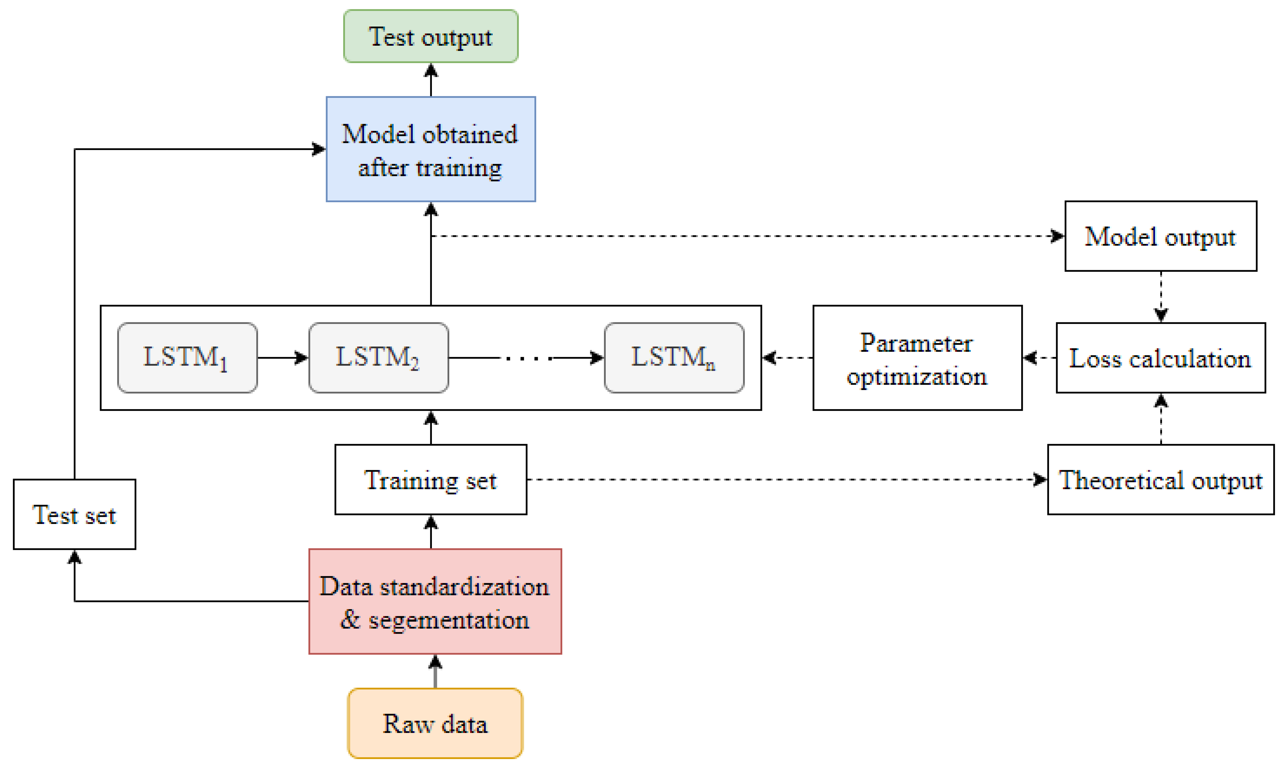Figure 14 depicts an LSTM-based fault diagnosis architecture.

The sluggish training pace of traditional RNNs is also of concern [82]. To address this issue, the literature [83] has proposed a fault detection method for asynchronous motors that combines RNN with dynamic Bayesian networks while also training the neural network using the simultaneous perturbation stochastic approximation (SPSA) method, which improves the training efficiency and fault diagnosis accuracy. A robust RNN adaptive gradient descent (RAGD) training technique was published in the literature [84], which considerably improves the RNN training speed. Using diagonal RNNs, the literature [68] presents a method for diagnosing interturn defects in the stator windings of asynchronous motors. RNNs with deviation units are used in the literature [69] to implement distortion voltage waveforms based on rectifiers. This method for diagnosing complex power electronic equipment or systems has been shown to be useful through fault classification and in experiments. An upgraded echo state network based on the RNN is applied to electromechanical systems in the literature [85].

3.5. Other Customized Deep Learning Methods

Despite the four conventional deep learning networks discussed above, researchers are still working to improve the detection method of occurring faults in electric machines and have developed several customized deep learning structures which showed a significant amount of perfection upon deploying to fault diagnosis. Chengjin et al. [86] have developed deep twin convolution neural networks with multidomain inputs (DTCNNMI) which builds three input layers so to integrate automatically extracted time domain, time–frequency domain, and hand-crafted time domain statistical characteristics, thereby resulting in improved model performance. The use of twin convolutional neural networks with large first layer kernels for extracting multidomain information from vibration signals is demonstrated, as is the resistance to the effects of ambient noise and changes in the operating circumstances on the final diagnostic findings. The efficacy of the suggested technique is demonstrated by comparing it to current representative algorithms and using experimental datasets. Taking into consideration the prospect of fault diagnosis under noisy environments, Dengyu et al. [87] have proposed a noisy domain adaptive marginal stacking denoising autoencoder (NDAmSDA) based on acoustic signals to mitigate the problem of domain shifting by introducing Transfer Component Analysis (TCA) and by speeding up the training process by replacing the traditional gradient decent of backpropagation with a forward closed-form solution, which enables the feasibility of reducing the difference between numerous noise levels as well as moving the classifiers from one noisy domain to others. An unsupervised deep learning network with mutual information (MI) [88], which is called deep mutual information maximization (DMIM), has been used to determine motor faults considering both global and local MI. The MIs between the output and multiple levels or areas of representations are estimated and maximized simultaneously using the f-divergence variational divergence estimation technique. It has been noted as a pioneer where a deep neural network input and output of mutual information has been maximized so to create a motor defect diagnosis model where the working environment is complex and noisy.

4. Discussion

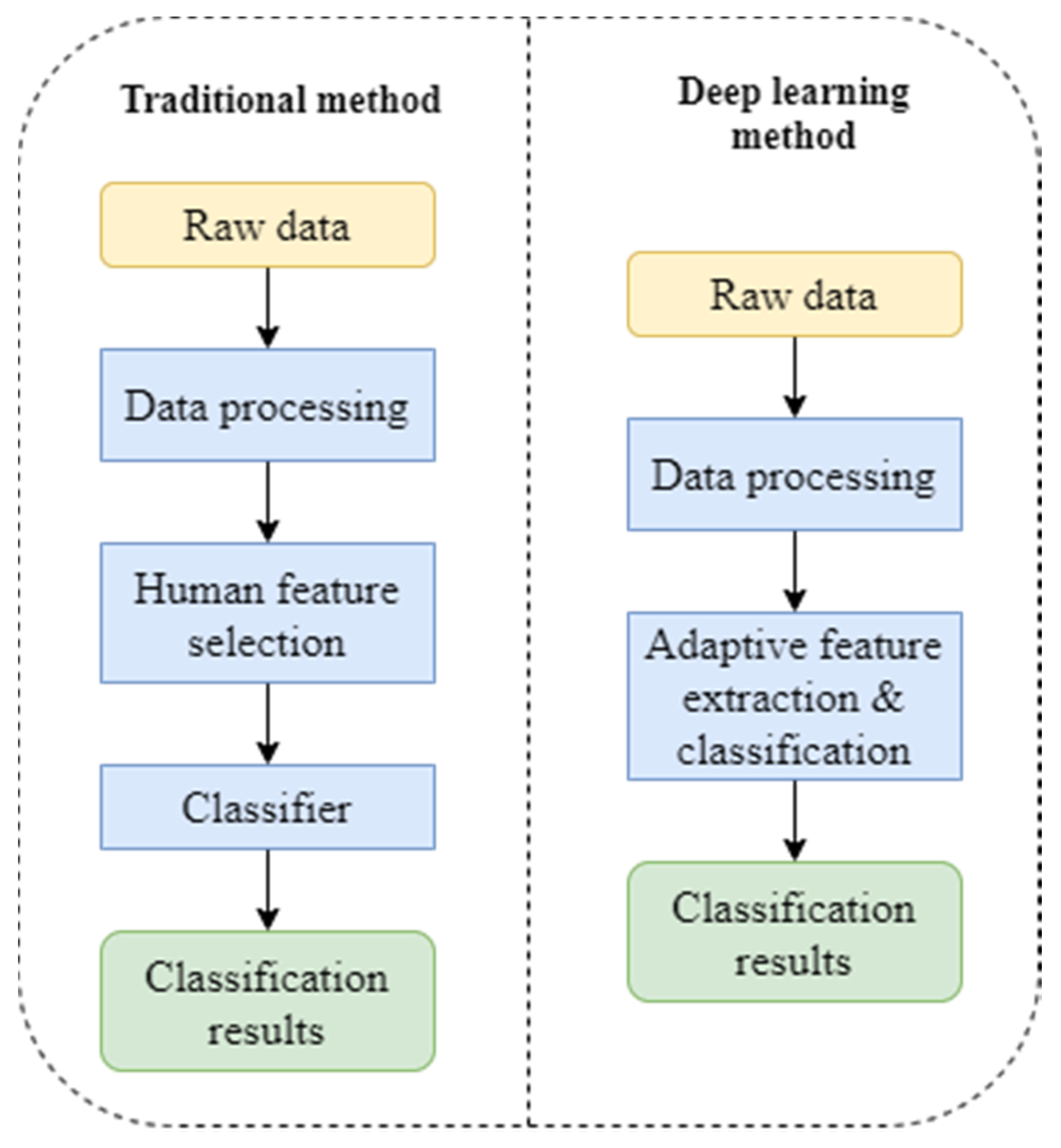
Many scholars have been drawn to the deep learning model because of the advantages it offers over traditional fault identification approaches. The most significant advantage of the deep learning model over the traditional feature extraction method is that it eliminates the uncertainty and complexity caused by human intervention [19], improves the intelligence of the recognition process, and of traditional fault diagnosis. A comparison of the traditional approach and the deep learning model analysis is presented in Figure 15.

Furthermore, each of the four types of deep learning models described in this article has its own set of benefits, which are summarized as follows:

(a)

Without a formal mathematical model, the DBN can learn data features adaptively [27]. The DBN multihidden layer structure efficiently avoids the dimensionality disaster problem. The inapplicability of the standard neural network training methods is effectively solved by the DBN semisupervised training method regarding multilayer network problems;

(b)

The Sparse AE facilitates the reduction of computational complexity and the generation of more concise features. The DAE can efficiently reduce the impact of random elements on signal extraction such as mechanical working conditions or external noise. The robustness of the stacked AE is improved;

(c)

The CNN offers tremendous mass data processing capabilities [89], as well as local perception, shared weights, and spatial or temporal downsampling, all of which help to lower network parameters and avoid network overfitting;

(d)

The RNN has significant applicability and improved accuracy in time series learning analysis [90], as well as in good dynamic system expression capacity.

Traditional fault diagnostic methods cannot match these benefits. These four types of deep learning models, on the other hand, have some flaws, which are outlined as follows:

(a)

The DBN uses a semisupervised training method in which each RBM is trained individually, and the parameters are adjusted layer-by-layer. As a result, the training will be much slower than in traditional defect diagnostic methods, and poor parameter selection will lead training to converge to a local optimum;

(b)

The Ordinary AE’s output and input are identical, making it susceptible to data overfitting during the mapping phase. Over-fitting can be avoided to some extent if the dimensionality of the hidden layer of the AE is smaller than the dimensionality of the input data, but this limits the characteristics that AE can represent, thus making reconstruction difficult. Deep AE can express more useful features, but it slows down the AE training time significantly;

(c)

The implementation of the CNN is relatively complicated, and the training of the CNN requires a lot of data, which also causes the training speed of the CNN to be very slow. For image processing, and due to the difference between the images and the industrial signals, the effect of the CNN in industrial applications is not very satisfactory. Therefore, there is relatively little research on the application of the CNN in motor fault diagnosis;

(d)

Gradient disappearance or explosion is a problem with ordinary RNNs. Although LSTM can help with this problem to some extent, it is more commonly utilized as a classifier. LSTM is only used in a few studies to achieve adaptive feature extraction.

In addition, the applicability of deep learning in motor problem detection is still in the early stages of research. There are still several issues with the four models discussed in this article, as well as other existing deep learning models:

(a)

While many classic machine learning algorithms have strong theoretical guarantees in particular contexts, current mathematical theories for deep learning are unable to provide a good quantitative explanation or theoretical foundation [91];

(b)

While the deep learning model’s deep network structure and powerful feature learning capabilities enable it to meet fault diagnosis in the context of “big data,” the deep learning model training speed is much slower than the linear model and is highly dependent on the training data set, and reports on optimizing deep learning training times are rare;

(c)

The number of hidden layers and the various parameters in the deep learning model must be selected based on experience and are easily affected by the input data, as reported by the existing literature. This is a problem that requires immediate attention;

(d)

Deep learning methods and classical defect diagnosis methods are not mutually exclusive. Some researchers are attempting to merge deep learning approaches with classic fault detection methods so to improve the diagnostic findings, but they are still far from achieving “mutual compatibility” [61].

After analyzing the methods, and with the help of the existing works of literature, we found that CNNs and RNNs are more suitable in the process of fault diagnosis due to their huge data processing ability and because they offer improved accuracy as well as dynamic system response capacity in detecting faults.

5. Challenges and Future Work

The difficulty of a deep learning model is connected to its design and training procedures. Despite the fact that there is a lot of literature on DL implementations in fault diagnosis systems, they require a previous understanding of the architecture. Deep learning is currently being developed using a variety of computer languages, including MATLAB, R, and Python. The diagnostic performance of the programming module may differ due to the different types of coding and training procedures. The architecture of the deep learning model has proven challenging to train during the previous few decades. The training process depends on characteristics of input data (i.e., the segmentation process, the size of the dataset, the parameters, and the hyperparameters of the deep learning algorithm). Real machinery system implementation is another big challenge in the fault diagnosis of electric motors. The majority of the deep learning applications accessible in public papers employ experimental datasets. There are just a few researchers that incorporate a genuine machinery system. An experimental dataset is acquired in a controlled environment with a less complicated system and less disruption to the situation. A genuine machinery system, on the other hand, is a complicated structure, and the data gathered includes information from several interrelated components of interest.

Many interesting directions in motor fault diagnosis are provided by deep learning, which has the potential to enhance the availability, safety, and cost-efficiency of complex industrial assets. However, there are a number of conditions that must be met by industry players before significant progress can be made. The automation and standardization of data gathering, notably the maintenance and inspection reports, and the implementation of data sharing across many stakeholders are among these needs, as are the potentially widely recognized methods of judging data quality. Moreover, the combined architecture of deep learning models with shallow machine learning algorithms, better ways to optimize hyperparameters, the measurement of remaining useful life (RUL), the incorporation of multiple sensors to collect data, and the analysis of fault visualization methods are the primary aspects that require further research.

6. Conclusions

This article highlights the current state of research on deep learning in electric motor fault diagnosis, as well as the benefits and drawbacks of the current deep learning models. Future improvements in theoretical research are expected to speed up the development of deep learning and provide greater instructions for both improving and using deep learning theories. This study will help scholars and respective maintenance engineers to better understand the general deep learning algorithms as state-of-art, and how they can be deployed to detect the faults of induction motors. Furthermore, this study varies in at least three significant ways from previous works in the literature. First, this study briefly represents the methodological structure of the four most generally used deep learning models, including their application to the fault diagnosis of induction motors which are used in manufacturing industries. Second, this article explores the application of the deep learning algorithms in detecting faults stepwise with an appropriate flowchart. Therefore, it will be easier for the maintenance engineers and technicians to review the methodology while applying a particular detection algorithm in the industrial sector. Third, this article provides a comparison between the traditional fault diagnosis methods and the deep learning models, exploring both the advantages and disadvantages. The limitations of these four models are also briefly discussed along with the existing methods. The challenges and the development of deep learning applications in motor fault diagnosis have been considered so to increase the operational time during unexpected breakdowns. It is clear that with the advancements in digital computational technology, deep learning models will remain powerful and appealing for use in fault diagnosis.