1. Introduction
The solution of many physical equations in fluid dynamics is generally obtained by discretesizing them into finite difference equations and then solving the algebraic equations. For complicated problems with high dimension or for the sake of accurate solutions, computational costs soar when more discrete points are required. This difficulty can be overcome by the increasingly popular and powerful machine learning approach. Machine learning is superior in dealing with any nonlinear problems compared to the conventional discretization method, which often requires making appropriate prior assumptions, performing linearization, and considering restrictive local time-stepping. Machine learning makes use of multilayer neural network architectures to model various physical systems. It has been acknowledged that standard multilayer feed-forward network architectures with sufficiently many hidden units act as universal approximators as they can approximate virtually any function to any desired degree of accuracy [
1]. The first attempt to apply neural networks (NNs) to solve PDEs was reported by Lee and Kang et al. [
2]. The main idea is to approximate the solution of PDEs using the NN as continuous functions and train the neural networks to minimize the solution residuals inside the domain and on the boundaries. Lagaris et al. [
3] demonstrated this idea by solving a number of benchmark problems such as the Poisson equation, subject to both Dirichlet and Neumann boundary conditions.
However, to solve differential equations with high accuracy, great care has to be taken when designing the neural network structure. Another challenge is that huge amounts of data have to be fed into the neural network in the training stage, which is a time-consuming and computationally prohibitive process. This prompts researchers to seek room for improvement: Is it possible to inform the neural network from the beginning for performance enhancement? Multilayer perceptions (MLP) was reported to build a smart neural model based on predicting the proper orthogonal decomposition modes of the Kuramoto–Sivashinsky (KS) equation and the Navier–Stokes equation [
4]. Karhunen–Loéve decomposition was applied to reduce the dataset for training of neural networks, after which the trained NN is capable of predicting the data coefficients at a future time. Similarly, MLP was also employed to compute the solution of the Stokes equation by decomposing it into multiple Poisson problems and then solving these Poisson equations with neural networks. The neural network approximates the Stokes equation using randomly sampled data points and delivers solutions that are in a differentiable and closed analytic form [
5].
Big progress was made by Raissi et al. as they introduced a new concept of ‘Physics Informed Neural Networks (PINNs)’ to tackle PDEs defined in complex domains with a variety of boundary conditions [
6,
7]. PINN exploits structured prior information to construct neural networks with physical equation integration [
8,
9,
10]. Gaussian process regression was employed to derive functional representations of linear and nonlinear problems. When dealing with nonlinear problems, locally linearization of nonlinear terms in time is required, thus limiting the methods applicable only to discrete-time domains. Furthermore, the method’s robustness is compromised with the Bayesian nature of Gaussian process regression as some certain prior assumptions are introduced. Inspired by the Galerkin method’s solution approximation strategy using linear combination of basis functions, K. Spiliopoulos et al. put forward that the solution can also been approached by the combined functions arising from vast number of neuron units in neural networks, and coined this approach the “Deep Galerkin Method (DGM)” [
11]. They also proved that the neural network would converge to the solution of the partial differential equation as the number of hidden units increases.
This idea was furthered by Lu and Karniadakis as they released the “DeepXDE” library to handle a wide range of differential equations including partial- and integro-differential equations [
12]. The concept of PINN was extended to solve problems with limited high-fidelity data and sufficient and readily low-fidelity data by constructing four fully-connected neural networks, which can learn both the linear and complex nonlinear correlations between high- and low-fidelity data. This work is pretty useful for high-dimensional regression and classification problems with large multi-fidelity data.
This paper is focused on developing a physics-informed, data-free deep neural network for surrogate modeling of various flow and heat transfer problems. A multi-layer neural network structure has been devised to approximate the solutions of physical equations, with the initial/boundary conditions being penalized in training stage. Compared with conventional data-driven machine learning approach, our devised neural network is advantageous as the training process is driven by minimizing the residuals of the governing equations, and no large labeled data from expensive numerical simulations are required. The generality and robustness of the proposed method are demonstrated in several flow dynamics and heat transfer problems. The rest of this paper is organized as follows.
Section 2 gives a comprehensive introduction of deep learning. The proposed physics-informed neural networks is described in
Section 3. In
Section 4, the developed approach is applied to solve a variety of test problems governed by various differential equations. Finally, the conclusion part in
Section 5 summarizes this work and points out the limitations and future directions of our method.
2. General Description of Deep Learning
Deep learning, a state-of-the-art method, has demonstrated its success in solving complex problems in speech recognition [
13], computer vision [
14], natural language processing [
15] and audio processing [
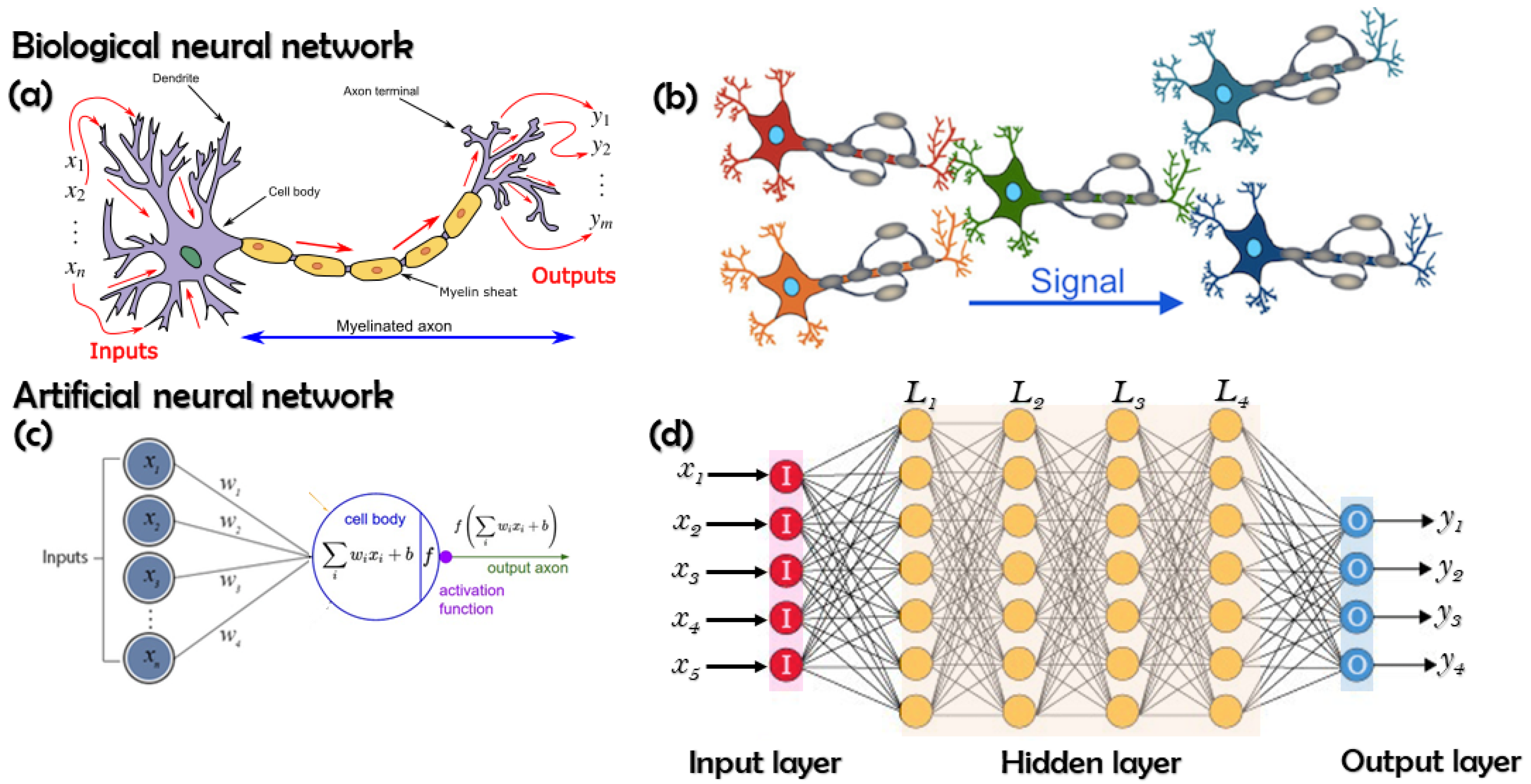
16]. It was originally inspired by biological neural networks, as is shown in
Figure 1. By mapping a large number of inputs into a target output, it can approximate and estimate highly complicated functions. As the neural networks go deeper, complicated features at various levels of abstraction can be learned and thus better predictability and higher accuracy are available. Increasing the number of layers enables neural networks to have superior generality as the level of features is enriched [
17]. With sufficient layers and enough transformations, neural networks are capable of approximating any function to any desired degree of accuracy. A systematical study by Chen et al. [
18] proved the universal capability of neural networks to approximate functionals, nonlinear operators and functions of multiple variables.
2.1. Deep Neural Networks
A deep neural network (DNN), a multi-layer neural network, is essentially a “stack” of nonlinear operations where each operation is prescribed by some adjustable parameters. Compared with single-layer neural network, a DNN can learn hierarchical representations to represent sophisticated phenomena as it has more parameters, more complex functions and better inductive bias [
19,
20]. Stacked layer by layer, deep learning is realized via such multi-layer neural networks, which act as the composite of nonlinear functions (also called activation functions) to transform function representation from one primary level into a higher, more abstract level (
Figure 1).
From the perspective of mathematicians, the multi-layered neural networks use the compositions of simple function to approximate complicated ones, and thus act as a compositional model regarding function representation. A deep neural network
with
N hidden layers is composed of a series of compositional functions, linear or nonlinear. A general DNN shown in
Figure 1d can be mathematically expressed as
where the symbol “∘” denotes function composition. Here
is the mapping from layer
to
N. The superscript “
in” and “
out” denote the input and output layer.
The N-hidden-layer DNN, denoted by
, implements the learning procedure by intaking the
d-dimensional data from the layer of input units at the bottom (
), mapping the incoming data via certain number of intermediate layers (
), and finally generating the
k-dimensional output from a layer of output unit at the top (
). The j-th layer has
neurons, with the associated weight matrix and bias vector being referred to as
, respectively. With the employment of activation function
, the
N-layer DNN is defined by:
The labeled training set consists of input vectors and output vector of length N. The free parameters are and explicitly write the neural network function parameterized by as .
2.2. Objective Function
In the training stage, the major task is to identify the optimal weights
that produce accurate predictions via the optimization of predefined objective functions, i.e., explicitly minimize a cost function by gradually adjusting the free-parameter weights. DNN acts as a mapping function
that approximates the true value
using the predicted value
. The cost is usually expressed as “Mean Squared Error (MSE)” defined in Euclidean space. The cost function is usually calculated as an average over all training examples, as is shown below:
where
is the mean squared error evaluated for the given set of N inputs
and the corresponding output
from neural network prediction.
2.3. Activation Function
The activation maps an incoming input
x to an outcoming output
y using different activation functions. Some of the most popular activation functions include Sigmoid (
), hyperbolic tangent (
), and Rectified Linear Unit (ReLU,
). The ReLU function accelerates the training process, making neural networks several times faster than their equivalents with tanh units [
21]. Another merit of ReLUs is that they do not require input normalization to prevent saturating. However, for regression applications, ReLU function suffers from diminishing second and higher-order derivatives, lowering the accuracy for cases involving such higher-order derivatives [
22]. Tanh or Sigmoid activations can overcome this issue brought by the second or higher-order PDEs. Moreover, sigmoids or Tanh are chosen for classification problems as they stretch the input space around a central point and can categorize elements into different classes.
2.4. Optimization Process
To train a neural network, the derivatives, mostly in the form of gradients and Hessians, need to be computed [
23]. Derivatives can be manually addressed as analytical formula, or computed by symbolic differentiation, numerical differentiation, and automatic differentiation (also called algorithmic differentiation, AD). The exact analytical expressions of derivatives are pretty hard to get manually for complex problems. More often, even if an analytical solution exists, its derivation is mathematically challenging, time consuming, and error prone. While for symbolic and finite differentiation, they both suffer from poor performance for complex functions [
24]. Hence, AD has become the mainstream for derivative calculations and serves as the real secret sauce that powers machine learning.
2.4.1. Automatic Diffraction for Derivative Evaluation
AD executes program codes and automatically computes derivatives using chain rule for accumulation of values instead of derivative expressions. Specifically, AD interprates computer programs by replacing the variable domains to incorporate derivative values and redefining the semantics of operators to propagate derivatives per the chain rule of differential calculus [
24]. For symbolic differentiation, the goal is a complex and accurate expression, whereas for AD, the goal is the numerical derivative evaluations. The main advantages of AD lie in its capability to evaluate derivatives at machine precision in constant time, with only a small constant factor of overhead and ideal asymptotic efficiency [
25]. Currently AD can be implemented in two distinct ways: Forward mode and reverse mode. Forward mode evaluates derivatives by transversing the chain rule from inside to outside. For instance, a general target function
f expressed in the composite of
k functions
where
, the calculation of derivatives in forward mode is:
While in the reverse mode, the dependent variable to be differentiated is fixed and the derivatives are calculated from outside to inside, as is shown below:
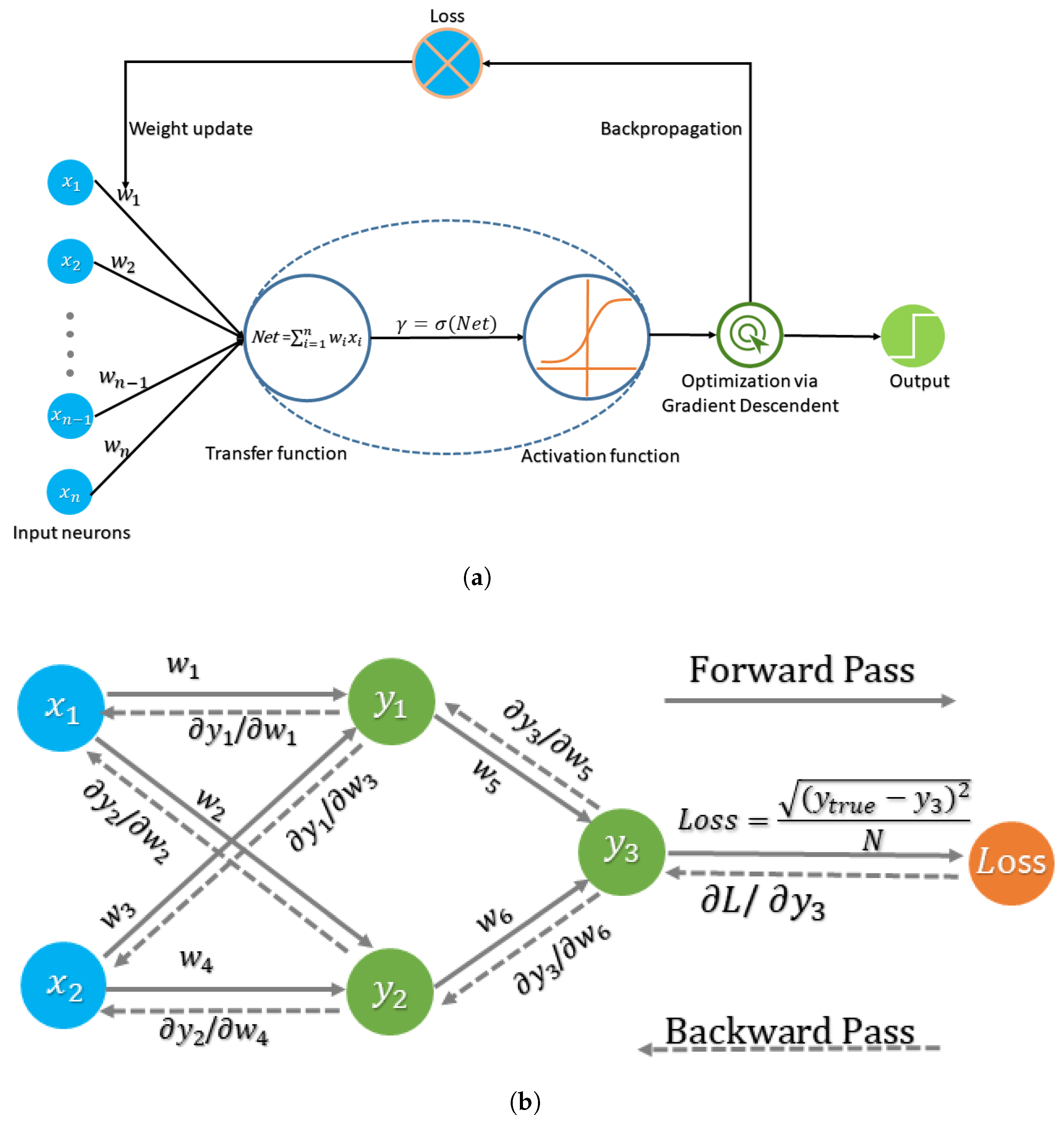
The backpropagation algorithm, a specialized counterpart of AD, is the backbone of neural network training. It is the method of fine-tuning the weights of a neural network based on the error rate obtained in the previous epoch (i.e., iteration). Proper tuning of the weights allows us to reduce error rates and make the model reliable by increasing its generalization. First the sensitivity of the objective value at the output is computed as partial derivatives of the objective function with respect to each weight utilizing the chain rule; then the sensitivity is backpropopagated to derive the required gradients. The process is essentially equivalent to transforming the network evaluation function composed with the objective function under reverse mode AD. At the heart of backpropagation is the partial derivative of the objective function with respect to any weight (or bias) in the network, which gives detailed insights into how the changing weights and biases change the overall behaviour of the network.
Figure 2 shows the role and key procedures of backpropagation in a simple neural network.
Figure 2b illustrates the phenomena, with an example describing both the forward and backward pass. In the forward direction, training inputs
are transformed to generate corresponding output
. A loss function measuring the error between predicted output
and the true value
is computed. For the backward propopagation, the sensitivity of objective function
with respect to different neuron weights
is used in a gradient-descent procedure for weights update.
2.4.2. Weight Update Using Gradient Descent
Gradient descent is commonly used to minimize an objective function with a combination of varied neural network weights . The minimization ends at a valley when following the downhill direction of the surface slope of the objective function. This minimization process updates the involved weights in the opposite direction of the gradient of the objective function with an assigned learning rate ; a hyperparameter controls how much the model weights are updated in response to the estimated error at each iteration. A small means a long training process that could get stuck, whereas a large value for the sake of accelerating the training process may prevent convergence due to the large fluctuation of loss function.
Based on the data used to compute the gradient of the objective function, the gradient descent algorithm can be classified into three variants: Batch gradient descent, stochastic gradient descent and mini-batch gradient descent. They show different levels of accuracy for the weight update and timescale at each iteration.
Batch gradient descent For the batch gradient descent (also referred to as vanilla gradient descent), the entire training datasets are used to compute the gradient of the cost function for parameter update. It will converge to the global minimum for convex error surfaces and to a local minimum for non-convex surfaces [
26].
Calculation of the gradients from the whole dataset makes the update quite slow and intractable for large datasets exceeding the memory limit. Batch gradient descent also does not support online model update, i.e., with new examples on the fly.
Stochastic gradient descent To prevent the slow convergence of batch gradient descent, stochastic gradient descent (SGD) has been introduced, where the fluctuations arising from the randomly selected points
allow jumps to new and potentially better local minima. This algorithm is a popular choice since it is fast, reliable, and has low susceptibility to bad local minima. In this algorithm, the weights are updated after the presentation of each example, according to the gradient of loss [
27].
By performing the update at each iteration, SGD converges much faster than its batch-based counterpart and enables the model to update online. However, the fluctuation of SGD makes its jump to local minima, complicating the convergence to global minimum. The fluctuation causes a sharp change for a large learning rate. Decreasing the learning rate slows the convergence of SGD, and its convergence history is similar to the batch gradient descent approach.
Mini-batch gradient descent To strike a balance between batch gradient descent and SGD, the parameter
is updated for every
n training samples
, coined as mini-batch. This mini-batch gradient descent reduces the variance of parameter updates, shows a stable convergence and is compatible with many state-of-the-art matrix optimization approaches. The mini-batch sizes can range from 50 to 256, depending on the application scenario. It has become the algorithm of choice and the term SGD usually refers to mini-batch gradient descent
It should be mentioned that this mini-batch gradient descent approach is also bounded by the challenge of getting trapped in some suboptimal local minima when minimizing highly non-convex error functions for many neural networks. This is because of the existence of saddle points which are usually surrounded by a plateau of the same error [
28]. The saddle points have one dimension slope up and another slope down; thus their gradients are close to zero in all dimensions.
3. Physics-Driven Deep Learning
In fluid dynamics, many transport phenomena can be modeled by some partial differential equations (PDEs), which can be expressed as
where
denotes a general differential operator consisting of temporal and spatial derivatives, as well as some linear and nonlinear terms. The position vector
is defined on a bounded continuous spatial domain
with the boundary denoted as
. The initial condition
and boundary condition
may contain differential, linear and nonlinear terms.
implements the Neumann, Dirichlet, Robin, or periodic boundary conditions. In view of that the true solution
is unknown or too costly to derive, an approximate one
can be obtained via the minimization of the cost function (usually the
norm of errors) with the following formula:
The training process of neural network produces a set of optimal
, which is calculated based on
With the initial and boundary conditions posed as constraints, the solution of the general nonlinear PDE (Equation (
11)) can be approximated as the outcome of the optimization problem defined by Equation (
13). To solve this optimization problem, the constraints in Equation (
13) are integrated into a sophisticated loss function that can be minimized by neural networks. For better illustration, the abstract PDE in Equation (
11) is reformulated in a more expressive way, as is shown below:
where the dimensional variable
. The unknown
is approximated by
from a well-crafted deep neural network with adjustable weights
. The accuracy of predictions is quantified by measuring the residual
of the equation satisfaction under the constraint of boundary and initial conditions:
where
and
is a positive probability density defined on the domain
.
The true solution for Equation (
14) can be identified under the condition of
. However, in real situations, it is pretty hard to derive
, especially for the high dimensional problems where the integral over the domain
is computationally intractable, hence a reliable approximate solution is sought at a reasonable cost. An approximate solution
should minimize the error indicator
. A deep neural network uses the stochastic gradient descent (SGD), an iterative method, to implement the minimization task. A key strength of SGD lies in its ease. SGD is simple to implement and also fast for problems with substantial training data, which reduces the computational burden, achieving faster iterations in trade for a slightly lower convergence rate [
29]. Instead of calculating the actual gradient from the entire dataset, the approximated gradient is generated by randomly selecting some data from the whole dataset [
30].
The overview of the whole procedure is shown in
Table 1. Key steps in solving the partial differential equations are listed below:
(1) Generate some random points
from
the probability density
to approximate the governing equation, Equation (
14). Moreover, sample another set of points
in
with the probability densities
to capture boundary condition Equation (
16) and pockets of random data
from
using possibility density
to meet initial condition Equation (
15). Lastly, distribute the random point
according to the probability density
. This sampling strategy avoids the lengthy and time-consuming mesh-generation process, and thus reduces computational cost.
(2) Calculate the objective function, i.e., the squared error
using the randomly sampled observation
:
(3) Explicitly apply the gradient descent algorithm to update the weights of neural network. Each iteration involves drawing an example
at random and applying the parameter update rule:
The “learning rate”
decreases with increasing iteration
n. It is either a positive scalar or a symmetric positive definite matrix. The step
is an unbiased estimate of
:
Therefore, the stochastic gradient descent algorithm will on average take steps in a descent direction for the objective function . The descent direction diminishes the objective function so that . As a result, the enables the neural network to produce a better estimation than .
As the iteration approaches to infinite (i.e.,
), the algorithm
would ultimately converge to the critical point defined as:
Since the stochastic gradient descent may converge to a local minimum for the non-convex optimization problems [
11], a caution must be taken that
is likely to converge to a local minimum rather than a global minimum for neural networks with non-convex nature.
4. Results
To illustrate the effectiveness of our proposed approach, four problems ranging from fluid dynamics to heat transfer are presented. These problems can be modeled by physical laws in the form of differential equations. To train the employed neural network, we use tanh as the activation function, and some other key hyperparameters are listed in
Table 2. Here, “Adam, L-BFGS” represents that the neural network was first optimized under the Adam algorithm for 1000 iterations, and then we switch to Limited-memory Broyden–Fletcher–Goldfarb–Shanno(L-BFGS) [
31] for the remaining iterations.
4.1. Potential Flow over Circular Cylinder
In this section, we present the application of the aforementioned algorithms to address the potential flow past cylinder problem. For this data-free approach, we do not need CFD calculated flow data used as inputs to calibrate the predicted results from neural networks. Instead, by exploiting the governing equation modeling the physical phenomena, we can ask the neural network to do self-learning by minimizing the customized errors instead of feeding them prior data used for supervised learning. Hence, if we know the governing equation, this method enables us to get rid of the lengthy and expensive CFD computations. It spins out neuron-generated solutions for the governing equations in a cheap and efficient way. Another big advantage of this promising technique that facilitates the study of various physical phenomena lies in the removal of the necessity of generating structural or non-structural meshes used for geometry discretion, which is a big challenge for modeling of transport phenomena in complex geometries.
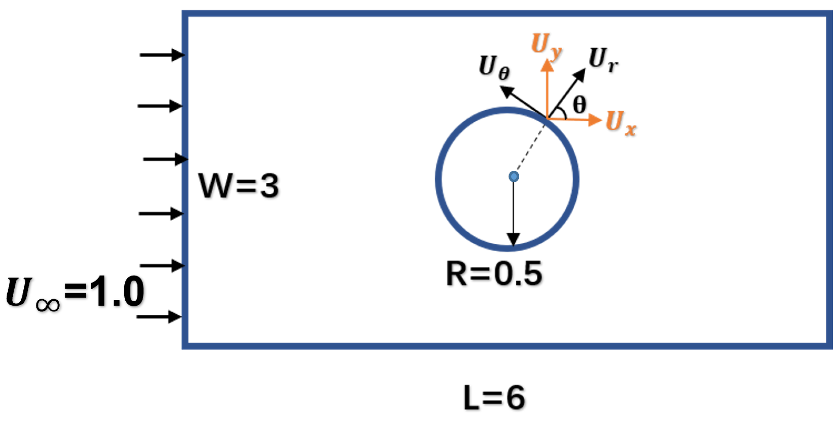
One of the most basic problems in elementary fluid dynamics is to find the velocity potential and streamlines associated with uniform irrotational flow past a cylindrical obstacle. This benchmark problem for stationary, inviscid, and incompressible flow has obvious application to simplified problems in aerodynamics. The test configuration considers a solid cylinder centered at (0, 0) with the radius
in a
by
rectangular channel. The fluid is assumed to have a constant density equal to 1.29. As the flow is assumed to be irrotational and steady; hence there exists a velocity potential
such that
where
is the velocity vector. The velocity components in the
x and
y directions can be obtained by
The relationship between potential and velocity can be expressed by Laplace’s equation as:
For a uniform flow with
, as shown in
Figure 3, the analytical solutions in Polar and Cartesian coordinates are
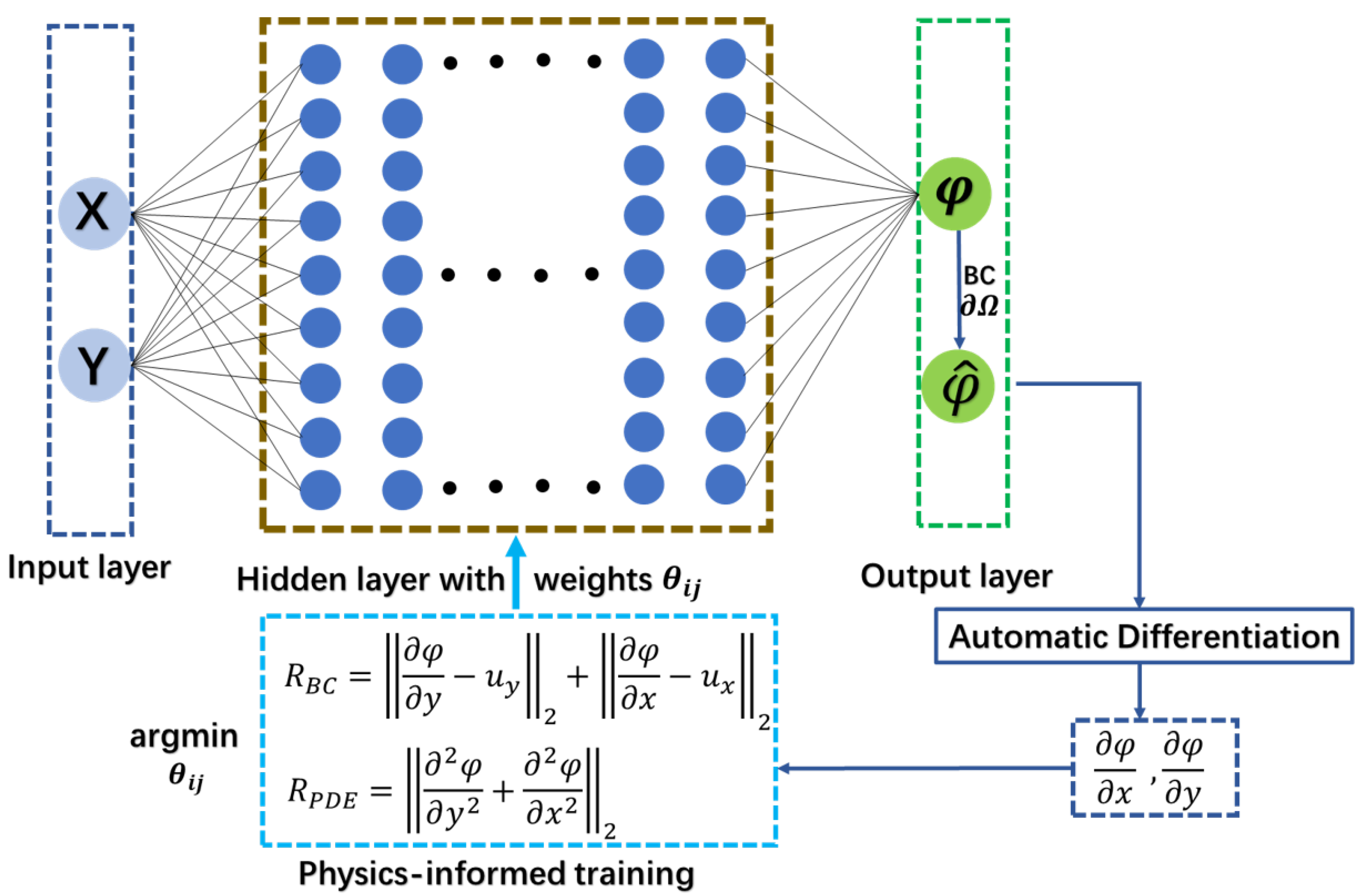
The designed neural network for this cylinder flow problem is shown in
Figure 4. Here the network consists of five hidden layers with each layer being 50 neurons. The Sigmoid function was chosen as the activation function.
is the residues of Laplace’s equation, which measures the difference between neural network predictions and the exact solution for each sampling data point. Meanwhile, the boundary conditions are considered by including the residual
, which quantifies the closeness of neural network predicted flows at each boundary to the imposed boundary conditions. Small values of both
and
are desirable. During the training process, both these residuals were minimized via the stochastic gradient descent algorithm. Ideally,
and
are expected to infinitely approach zero. In reality, it is generally accepted that an extremely small value, say
, indicates the converged and reliable prediction results.
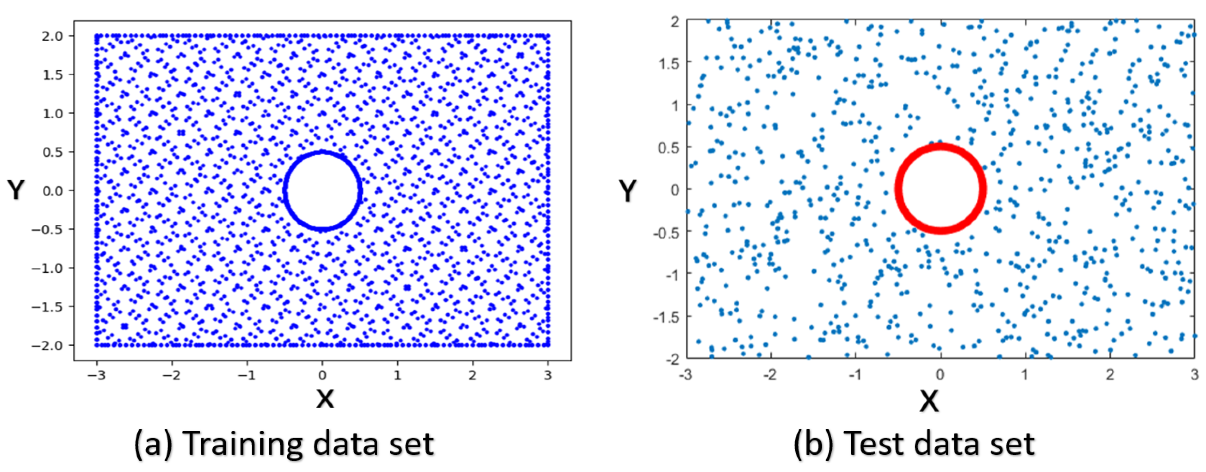
To approximate the flow field inside the computational domain, 2000 spatial points were randomly sampled inside the domain, as is shown in
Figure 5. Here the predicted flow field is used to evaluate how well it satisfies the Laplacian equation. The residue
at each point was summed up to quantify the deviation of the prediction from true solutions. The satisfaction of the imposed boundary conditions was evaluated at the 400 data points sampled at the boundaries, i.e., the left, right, bottom and top boundary of the rectangular domain and the surface of the cylinder.
With 30,000 iterations, the training loss was reduced to the magnitude of
. To test the accuracy of the network’s prediction capacity, 800 randomly sampled spatial points were used, as shown in
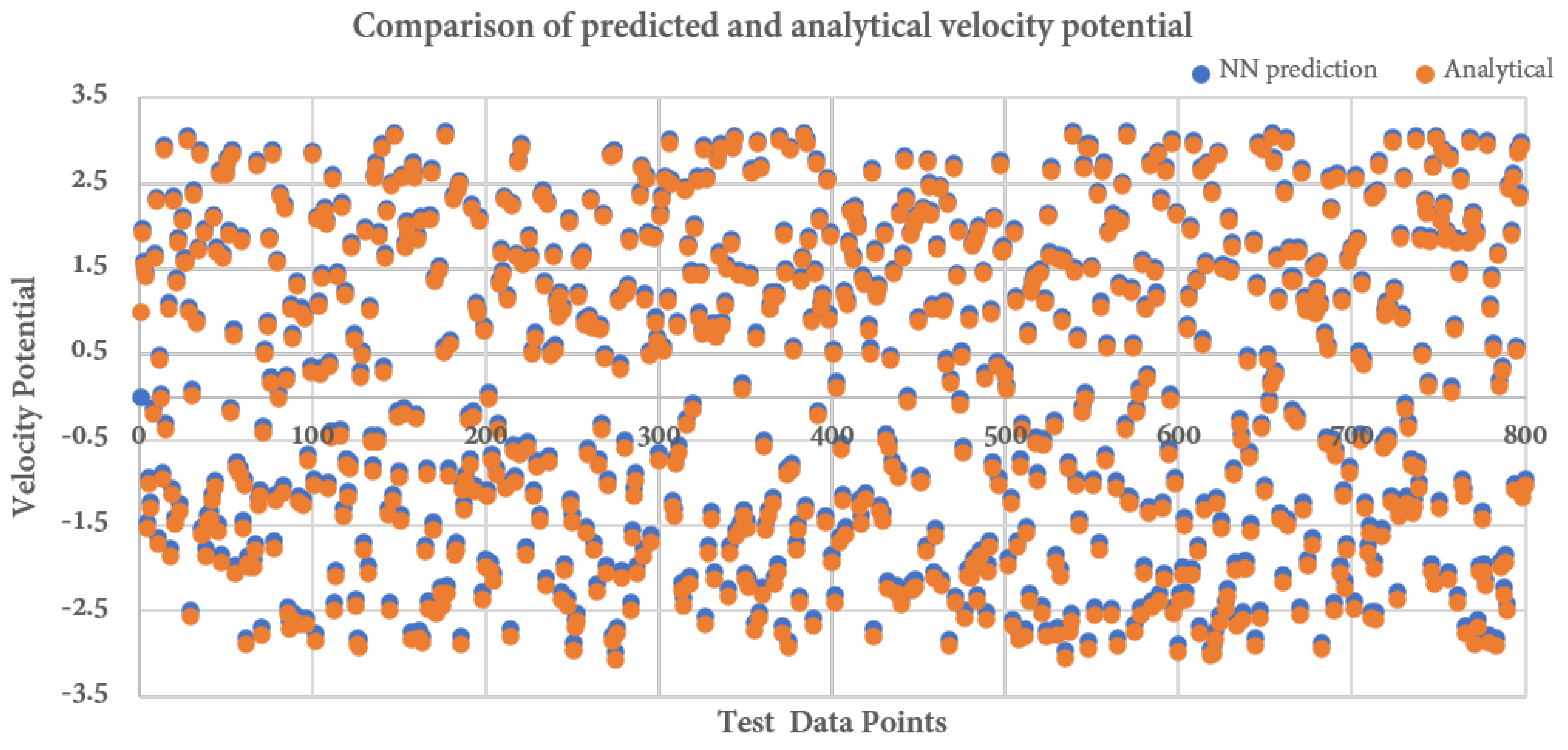
Figure 5. The predicted flow potential is shown in
Figure 6. The coincidence between blue and orange points indicates the predicted results approximate the analytical results with high accuracy. The deviation between these two datasets is the source of the prediction error. As to our concern, the neural network gives a pretty good prediction, as indicated by the small deviations between these test points.
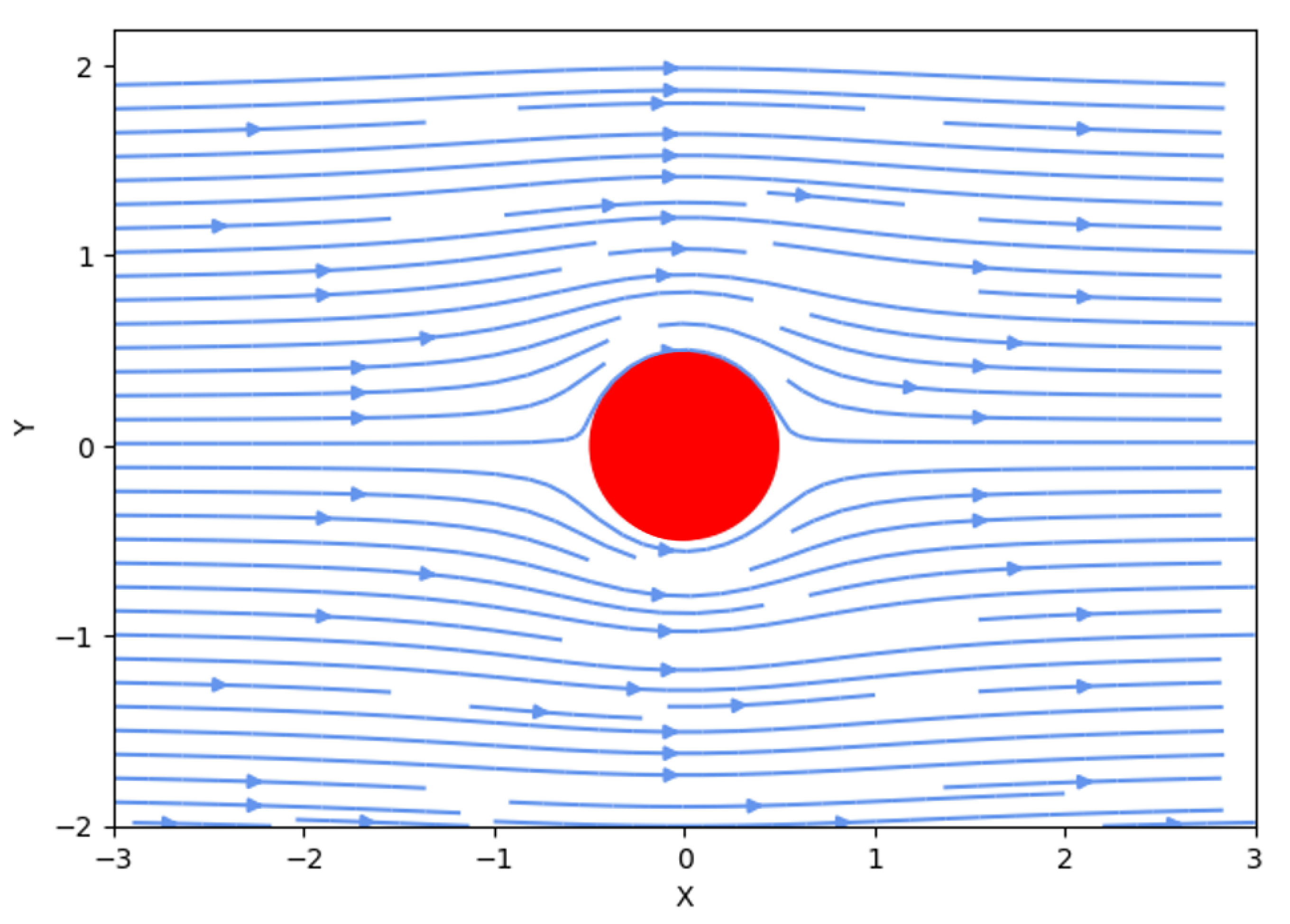
Further evidence including streamline and vector field is also provided to double check the outcomes of the neural network predictions.
Figure 7 and
Figure 8 show the streamline and velocity field predicted by the employed neural network. The velocity magnitude exhibits two lines of symmetry. A line drawn horizontally through the cylinder divides the velocity magnitude into upper and lower sides that are geometric mirror images. Note that the velocity itself is not symmetric about this line. These results lead to the conclusion that the employed neural network has excellent capacity to predict this flow phenomenon with high accuracy.
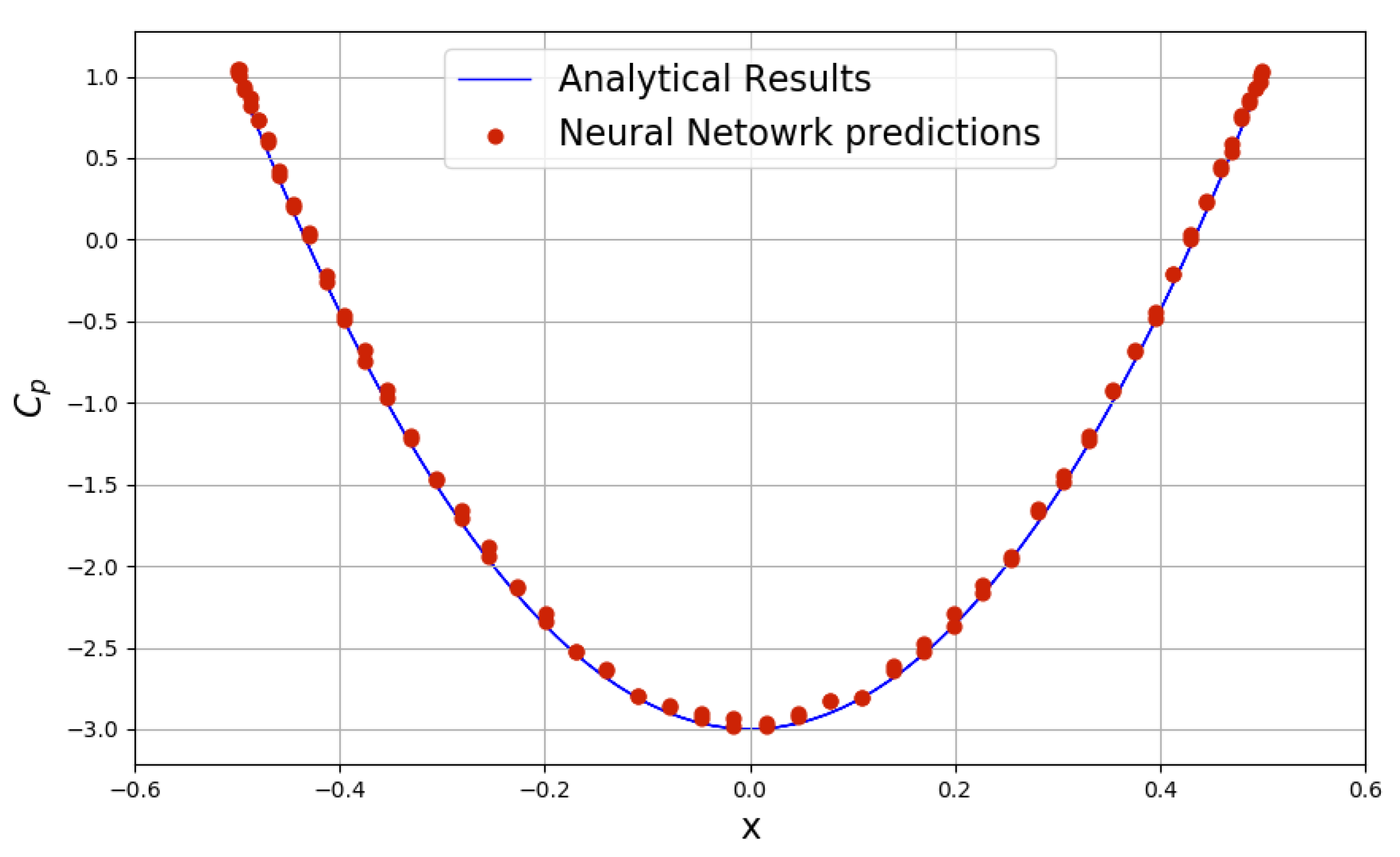
Using Bernoulli’s equation, we can obtain the pressure coefficient
Even if this inviscid flow case is simple, the predicted results can enable people to have good estimates of the pressure and velocity distribution as the pressure and velocity distribution are related via Bernoulli’s equation. It should be noted that for real fluid flows past a cylinder, we have to consider viscous effects, which cause the flow to separate away from the cylinder, and the streamlines are no longer attached to the cylinder body.
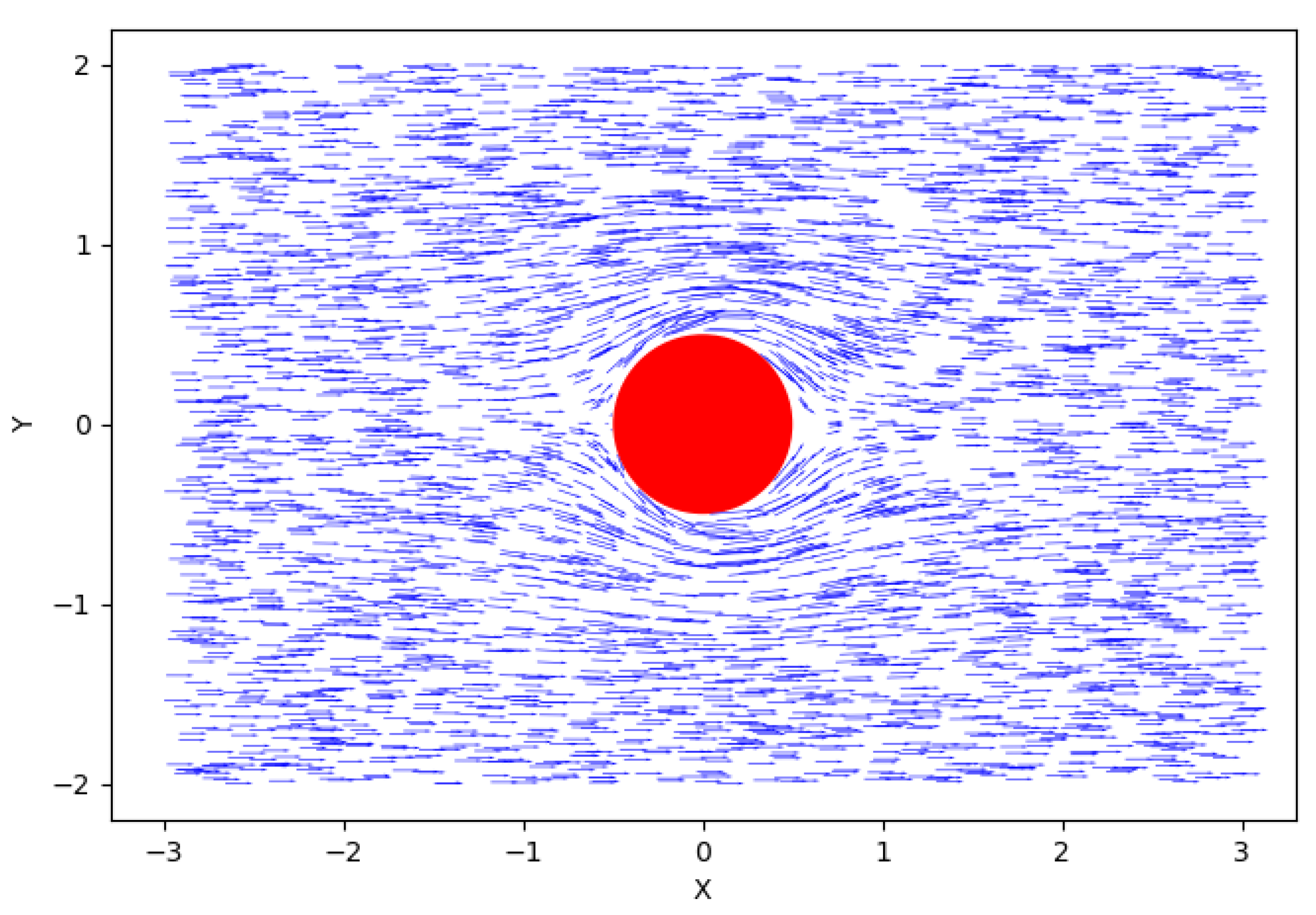
Figure 8 shows predicted flow velocity. From this figure, we know that along the surface of the cylinder, flow velocity is in a tangential direction, i.e., parallel to the surface of the cylinder. As the mainstream flow gets close to the cylinder, fluid elements begin to decelerate. There is a stagnation point as the fluid element on the surface of the upstream side of the cylinder is stopped. Due to the zero velocity at stagnation point, pressure increases to its maximum value, while the pressure coefficient reaches its maximum.
Figure 9 shows the pressure coefficient distribution along the cylinder surface. The estimated pressure coefficients from neural networks match well with the analytical results. For fluid elements passing either above or below the cylinder, their velocity magnitudes increase due to the narrowing flow path. For this inviscid flow, flow velocity decreases as flow continues around the downstream side of the cylinder, producing a second stagnation point at the downstream equator. Further downstream, flow velocity begins to increase and gradually returns to the free stream value.
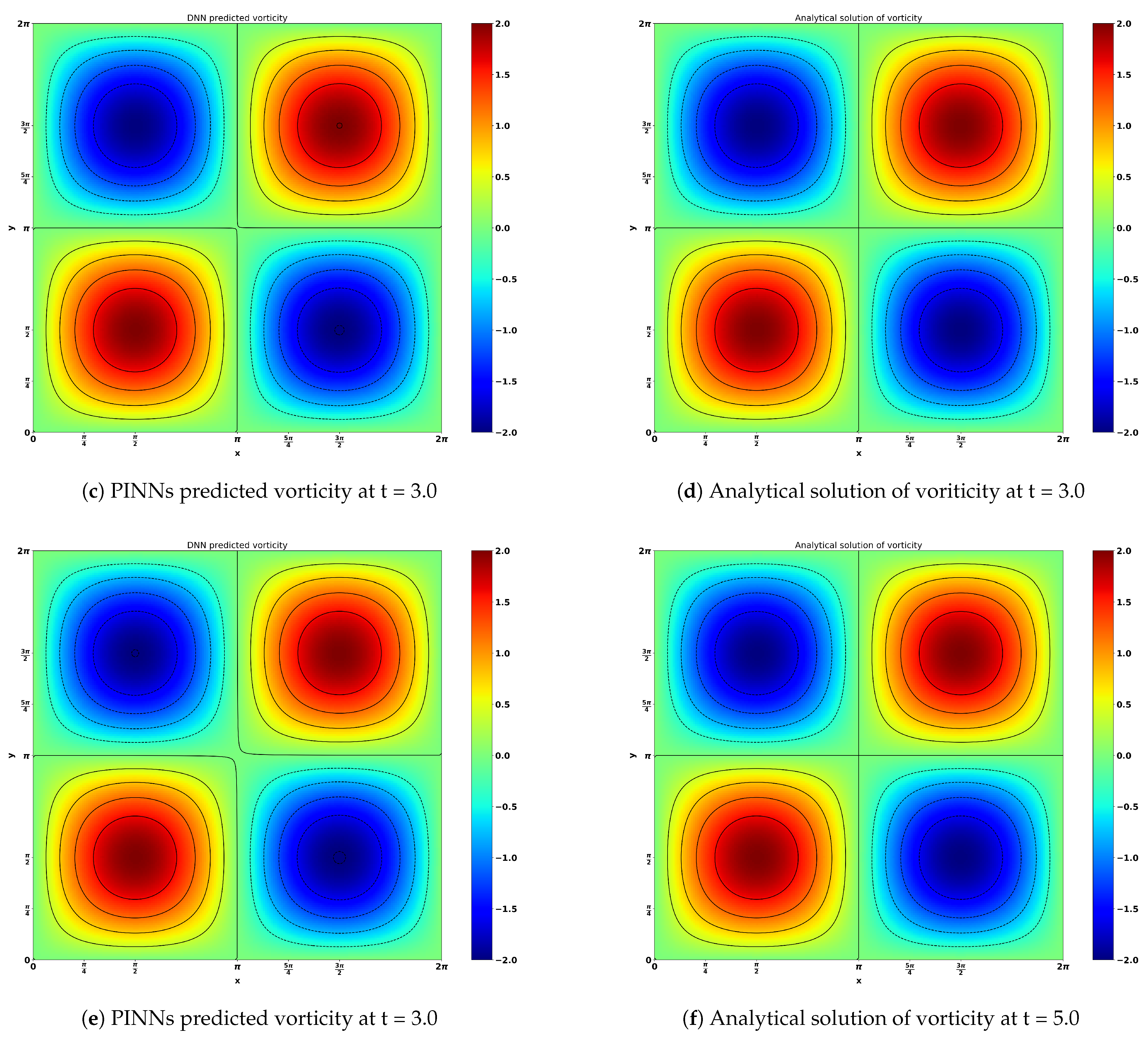
4.2. Taylor–Green Vortex
The Taylor–Green Vortex (TGV) is an unsteady flow of a decaying vortex and was firstly solved by Taylor and Green by a perturbation series in time to explain the creation of small scales by vortex-stretching, diffusion, and dissipation in a three-dimensional (3D) flow field [
32]. It has an analytical solution based on the incompressible Navier–Stokes equations in Cartesian coordinates and thus is widely used as a benchmark problem in validating solvers and formulations in numerical computations. Here the two-dimensional decaying vortex defined in the square domain,
serves as a benchmark problem for testing and validation of incompressible Navier–Stokes codes.
Without the presence of body force, the incompressible Navier–Stokes equation in the Cartesian coordinate system is given by:
In the domain
, the solution is given by [
33]:
where
is the kinematic viscosity of the fluid. The pressure field
p can be obtained by substituting the velocity solution in the momentum equations and is given by
The stream function satisfying
and the vorticity governed by
can be expressed by the following equations:
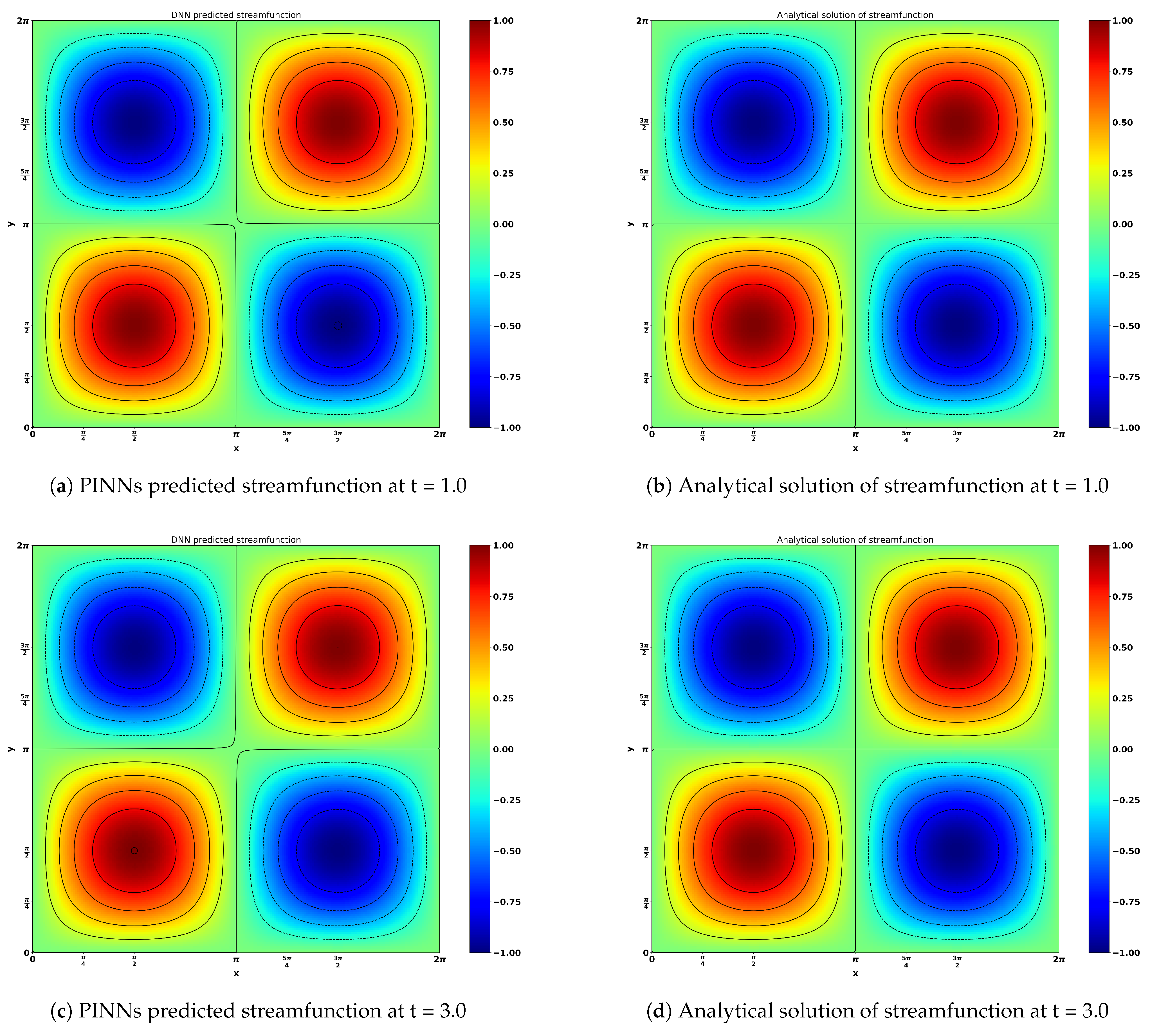
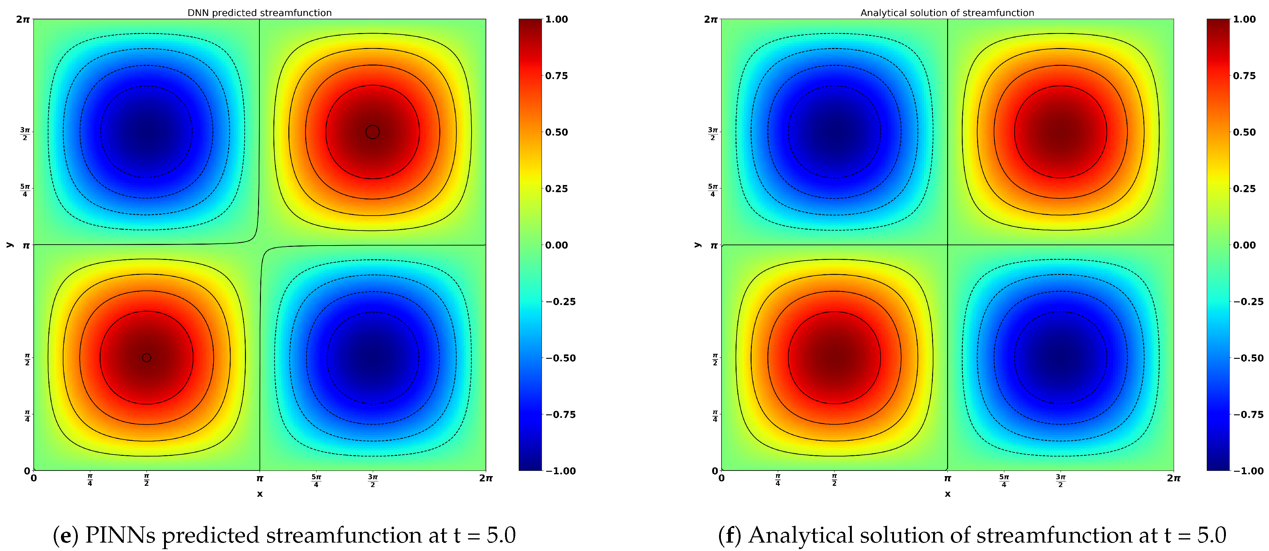
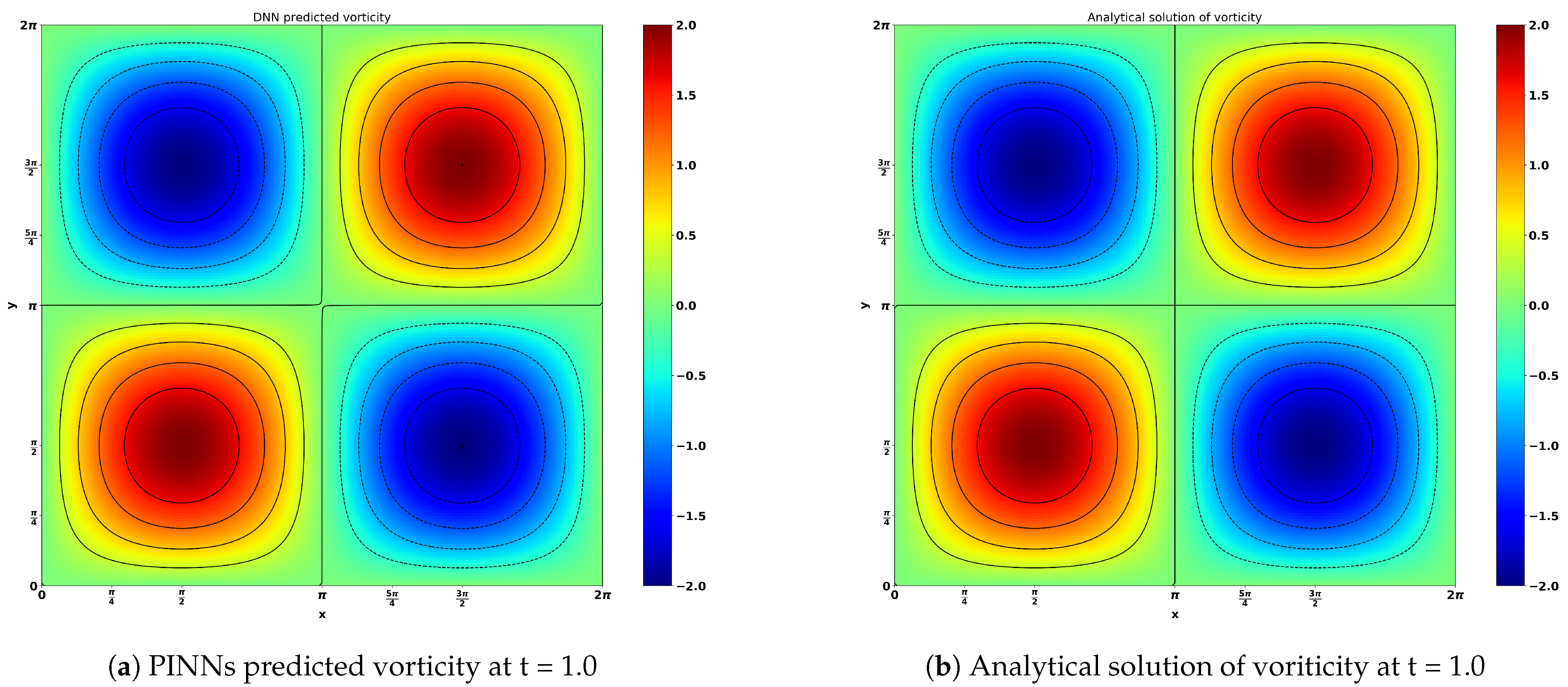
The neural network predictions were trained using 2000 residual points that are randomly sampled in the spatio-temporal domain, and 300 and 600 points for the initial and boundary conditions, respectively.
Figure 10 shows the result obtained by neural network predictions and analytical solutions of the viscous Navier–Stokes equation for the Taylor–Green vortex flow. The time evolutions (t = 1.0, 3.0 and 5.0) of the stream function and vorticity are presented in
Figure 11a,b, respectively. There is a negligible difference between the neural network predicted results and the analytical solutions. This great consistency showcases the excellent capacity of neural networks for flow predictions.
The above figures also show multiple well-defined laminar vortices and their interactions and evolutions in time. The TGV flow is initially characterized by the set of laminar, well-defined, and symmetric vortices, which evolve and interact in time, leading to vortex stretching mechanisms generating vortex sheets which gradually get closer. In summary, this study reinforces the potential of the proposed machine learning method to calculate transitional flows of practical interest efficiently [
34]. Our approach provides an efficient computational alternative to allow scientists and engineers to use this TGV flow as a test-case to study more complicated transition to turbulence driven by vortex-stretching and reconnection mechanisms.
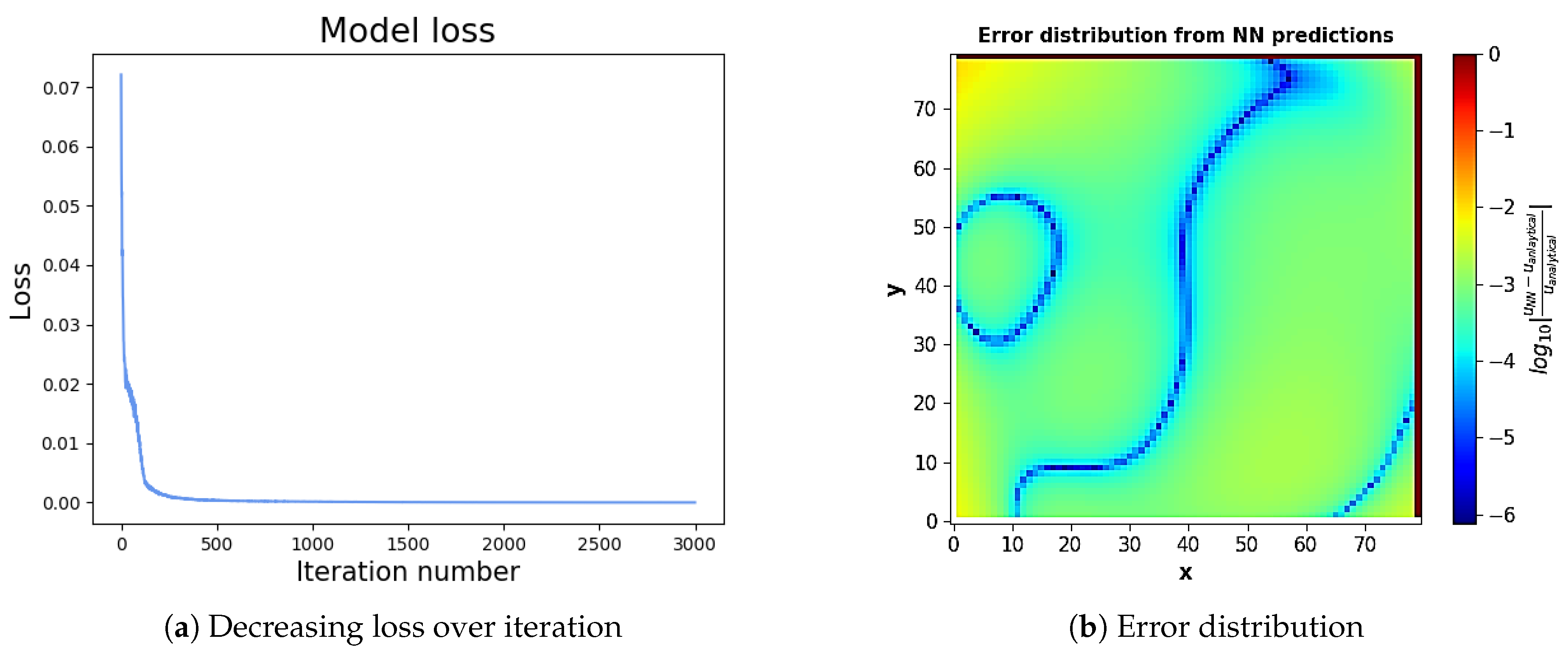
4.3. Linear Poisson Problem
The accuracy and efficiency of the proposed technique were tested in the following two-dimensional inhomogeneous partial differential equation:
along the whole squared boundary. In this case, we use a network of five layers with 30 neurons on each layer to predict flow potential
. The physical law and boundary conditions (Equation (
32)) were incorporated into the designed neural networks. After training, the loss history and prediction error distribution are shown in
Figure 12. This error plot is calculated based on the relative difference between the PINN predictions and the analytical solutions presented in Equation (
33). The error contours show that the achieved mean errors are around
and the minimal error can be as small as
.
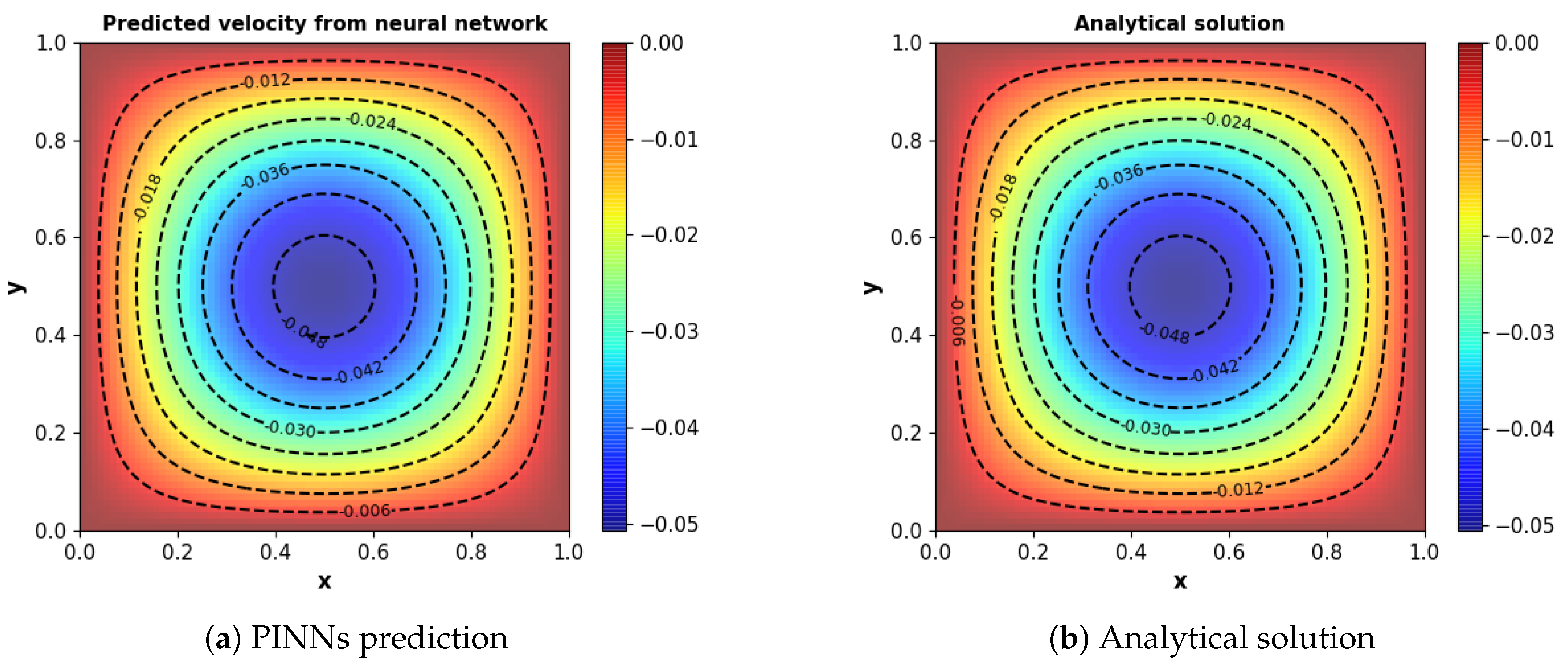
The analytic solution is found to be
The accuracy of network predictions can be clearly illustrated as in
Figure 13 by comparing the contour plot of PINN predicted unknown
u and analytical solutions. Differences can be hardly spotted as the prediction accuracy is high enough. Meanwhile, the isovalue lines of
u value, as represented by the dashed dark lines, are superposed onto the contour plot to quantify the parameter distribution as well as for better visualization.
In this problem,
is a scalar potential which is to be determined, and the right-hand side of Equation (
32) is a specific source function. Poisson’s equation shows linear property in both the potential and the source term; hence its solutions are completely superposable. Moreover,
Figure 13 shows that equipotential sets of the solution graph become smoother as the potential increases.
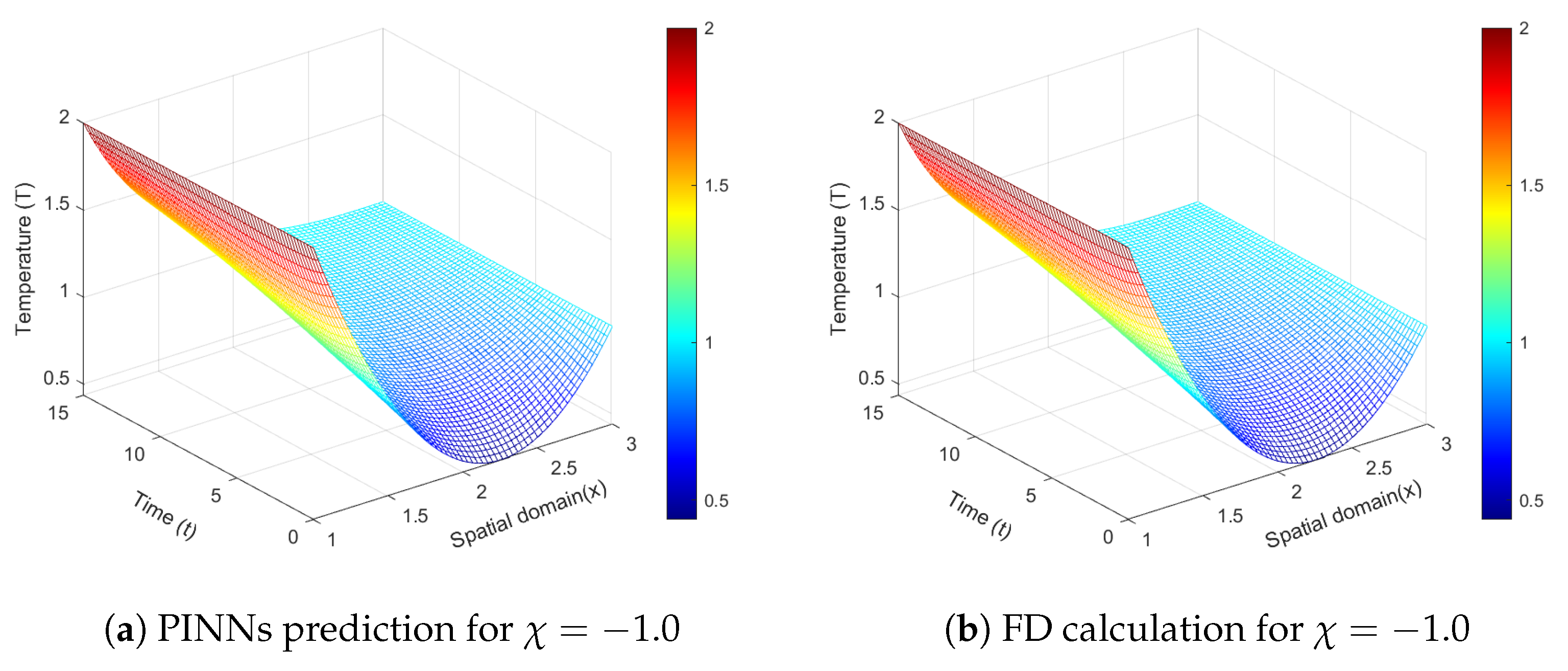
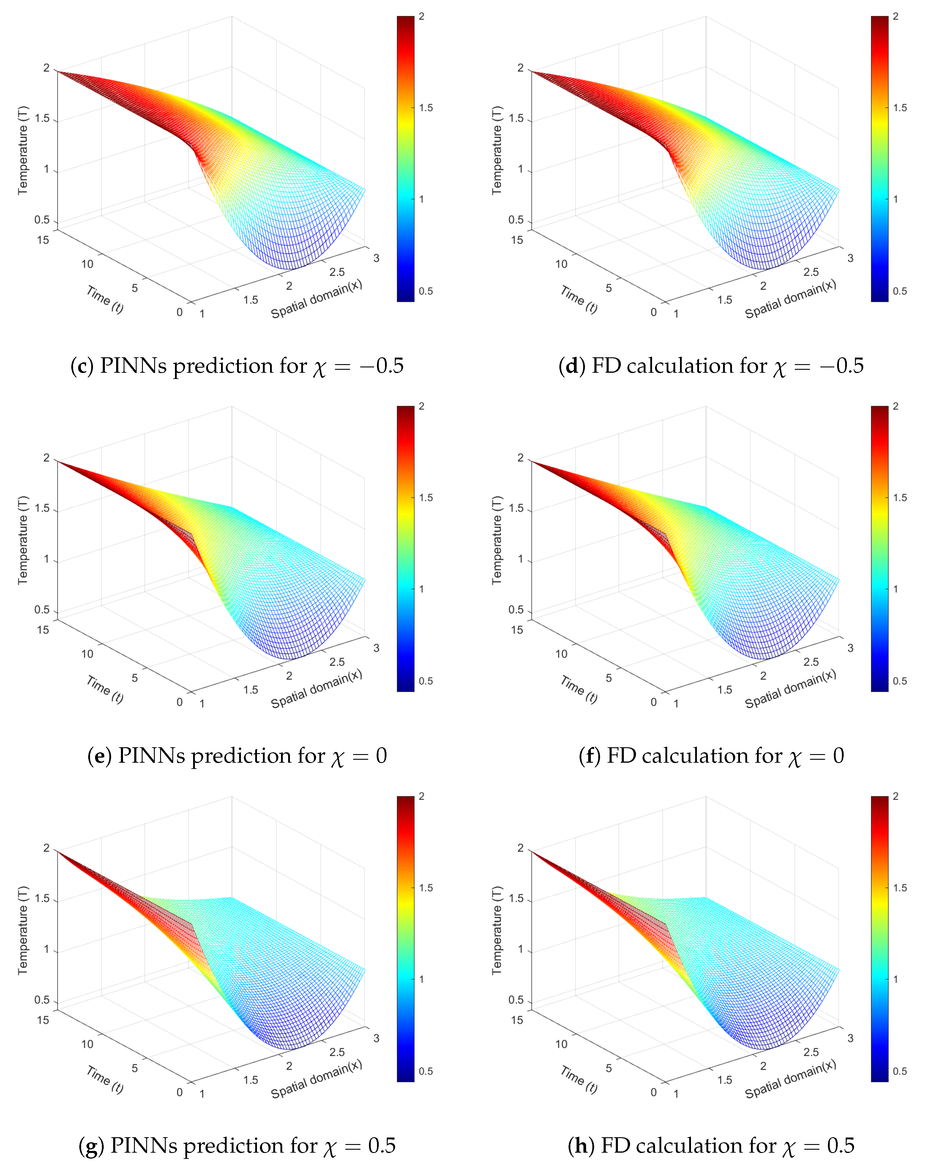
4.4. Thermal Conduction with Non-Linear Heat Generation
The capability of the developed neural network scheme for non-linear problems is also illustrated by a non-linear heat generation problem, where an unsteady temperature distribution in a homogeneous solid is predicted. Temperature field is governed by the following equation:
where the
is the temperature at point
x and time t,
is the density,
is the heat capacity under constant pressure, and
is the thermal conductivity of the selected media. Here
and
are assumed to be constants while
varies with medium temperature. After some differential operation, Equation (
34) is transformed into the following form:
If
takes a constant value, i.e.,
, then Equation (
35) becomes a linear (parabolic) partial differential equation. In contrast, when
, the Equation (
35) is nonlinear, which can be solved numerically. For this initial-value (Cauchy) problem, the finite difference method is used for solution derivation with the implicit Euler scheme employed for temporal discretization [
35].
For illustration, the thermal conductivity is assumed to have the form of
. The constant parameters have the value of
. The spatial domain
includes a boundary condition
The initial condition of temperature is
With the aforementioned boundary and initial conditions, the time evolution of Equation (
35) can be solved.
Figure 14 shows both the results from neural network predictions and the numerical computations using finite difference (FD) method [
35].
5. Conclusions
This paper presents a new solution framework based on physics-constrained machine learning that can be used to solve partial differential equations in fluid dynamics and thermodynamics. By leveraging prior physical laws, our feed-forward fully-connected neural networks are capable of solving physical equations commonly seen in fluid dynamics efficiently. Instead of using collocation points to discretize the spatial and temporal domains to find solutions, randomly sampled points were employed to evaluate their satisfactions of the desired physical equations. Automatic differentiation was adopted to handle differential operators, enabling this approach to be mesh free and time efficient. Since random points are generated on spatial domains, this randomness helps to capture complex physics in irregular computational domains. Thus, this mesh-free method is particularly attractive for problems with complex computations domains. The approximate solutions satisfying the differential operator can be obtained via tuning the deep neural network parameters, which are trained by minimizing the squared residuals over the entire computational domain. In particular, the initial and boundary conditions are satisfied in a weak sense by imposing related penalty terms to the loss function. This modified loss function is used as the objective for minimization. The effectiveness and robustness of this proposed method have been illustrated via solving the flow past cylinder problem, linear Poisson problem, heat conduction and Taylor–Green vortex problems. The proposed method is relatively simple to implement, and provides a good tool for engineers and scientists to develop, test, and analyze their ideas.
While the proposed PINNs have great potential as an alternative solver for some physical problems, there is a long way to go to replace the traditional numerical method. For real problems with a large and complex computational domain, PINNs are still slower than the finite element method. Another challenge lies in their incapacity to address some multi-physics and multi-scale problems, which typically require heavy computations. Last but not the least, the design and construction of effective neural network architectures remain to be a headache as different users may build different neural network structures, which unquestionably imposes substantial impacts on the performance of PINNs as well as the accuracy of the predicted results. As further extensions to this work, we aim to tackle these challenges to facilitate this physics-based machine learning approach to tackle more complex problems in thermodynamic fluid dynamics. We will use emerging meta-learning techniques to automate the design of more efficient neural network structures and propose some customized loss functions for different tasks.


