Traveling Wave Energy Analysis of Faults on Power Distribution Systems

Abstract

This paper explores the most important factors that define the Traveling Wave (TW) propagation on distribution systems. The factors considered in this work are: the distance to the fault location, the fault type, and the crossing of system elements (such as regulators, capacitor banks, laterals, and extra loads within the protection zones). This work uses a realistic, yet simplified, distribution system composed of two protection zones, in which, several combinations of the previously mentioned factors are considered. The simulated fault measurements undergo a signal processing stage in which, first, they are decomposed into independent modes using the Karrenbauer transform. Second, a time–frequency representation is obtained using the Stationary Wavelet Transform (SWT), dividing the signal into several frequency bands. Finally, the Parseval’s Energy (PE) theorem is applied to calculate the signal energy in each frequency band. A qualitative analysis is performed based on the previously calculated energies to outline which are the factors that most affect the TW energy during propagation. The results show that distance, the presence of regulators, either in the propagation path or upstream, and the type of fault are the main factors that affect TW propagation across the system, and therefore they should be considered for TW-based protection schemes for distribution systems.

1. Introduction

The application of Traveling Wave (TW)-based protection schemes is one of the main challenges in the distribution network in years to come. A notorious effort is being made in this regard for a worthy outcome: locating faults in a sub-cycle fashion. Once achieved, this will open a new protection paradigm and will be beneficial to the system and to the components that depend on it. Different groups of techniques can be applied to obtain information of the first microseconds after a fault occurs [1]. Multiple algorithms have been designed to perform fault location and classification using extremely short portions of the data [2,3]. This paper does not aim to provide a fault location method, but to provide an in-depth explanation of the fault signatures in the dozens of microseconds that follow a fault detection. The main purpose of this work is to provide a variety of insights to foster further research that will eventually serve as the basis of future fault location methods. Analyzing and understanding these fault signatures gives useful information on how TW-based protection methods could work for distribution systems, and how the challenges could be addressed.

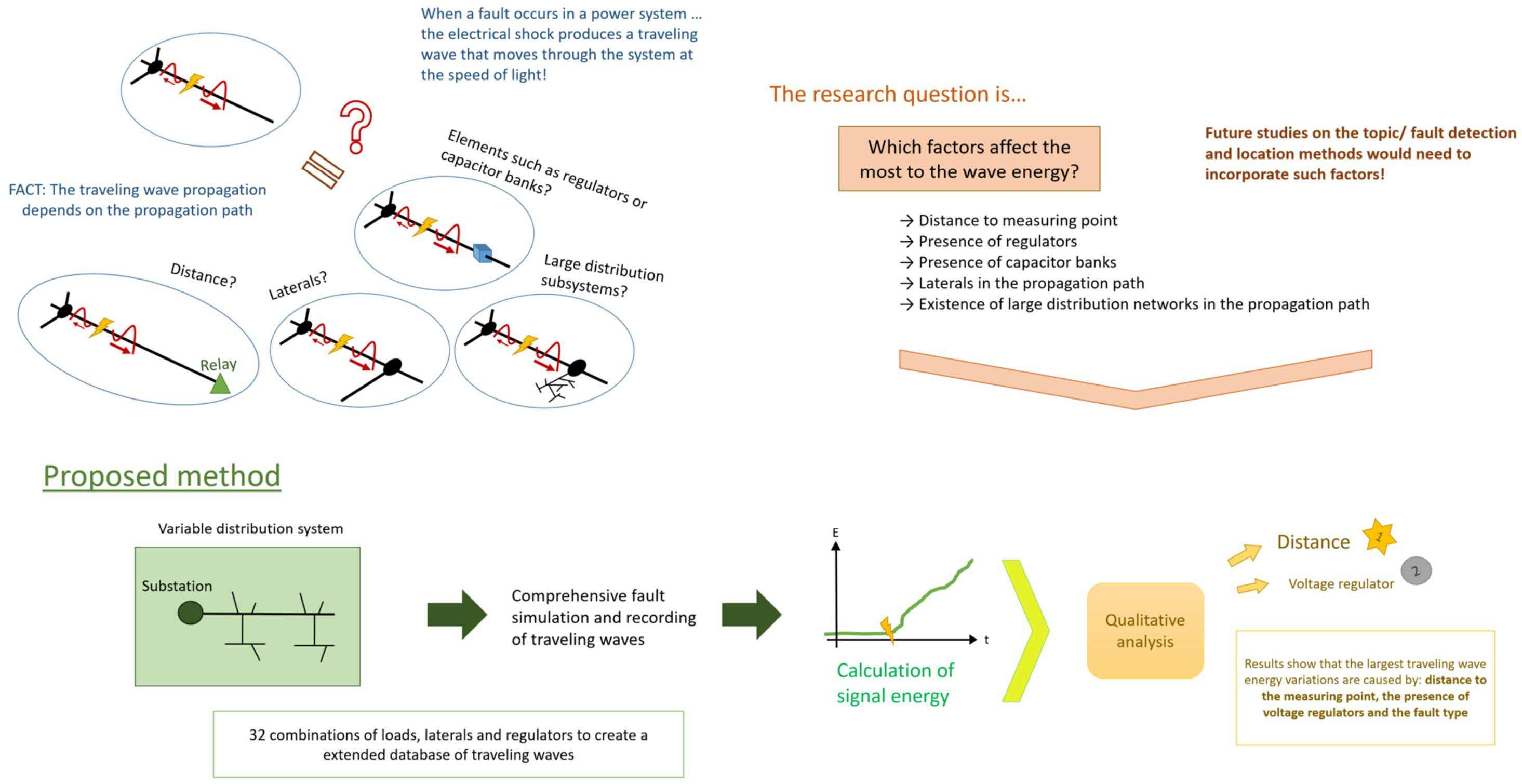
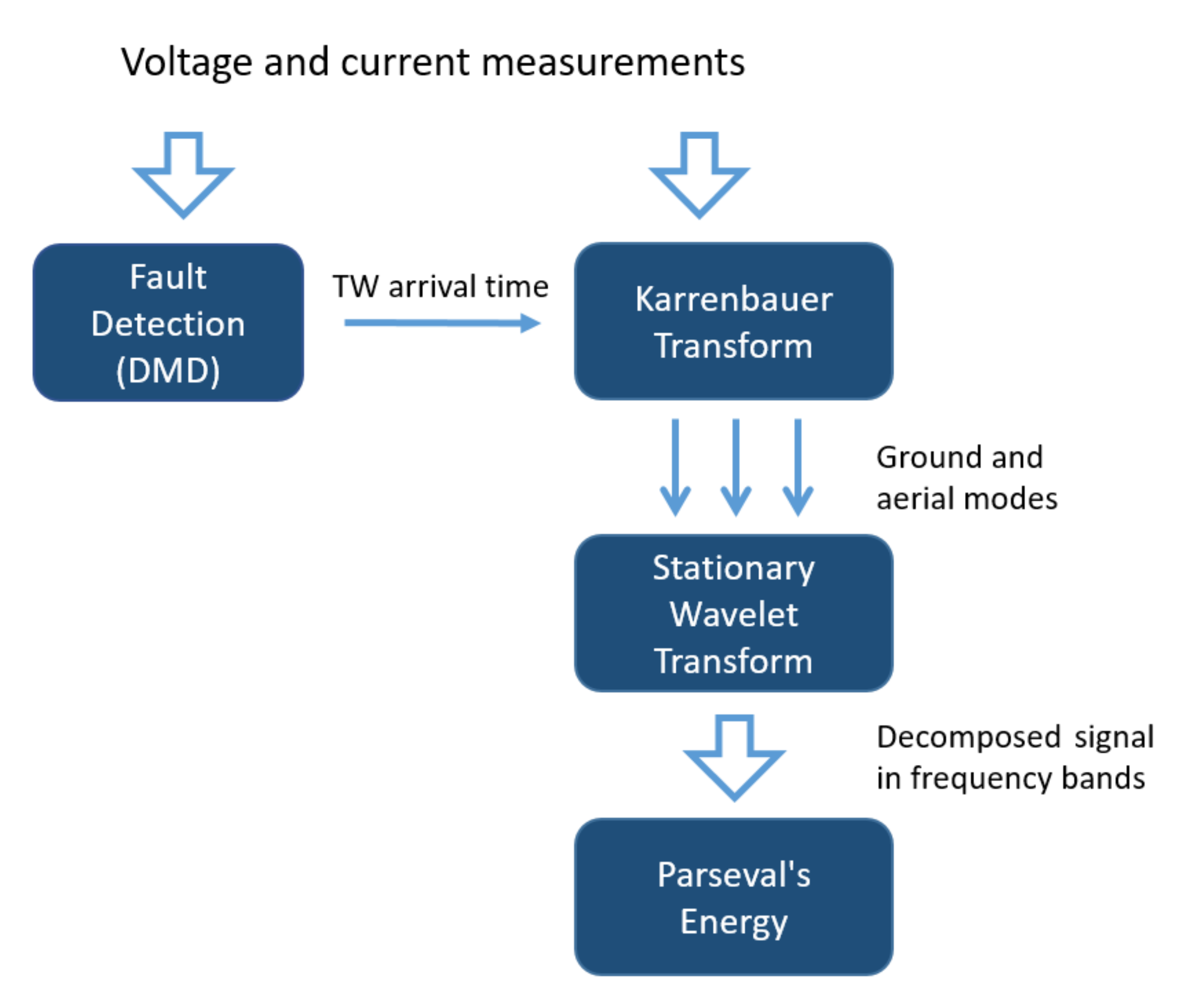
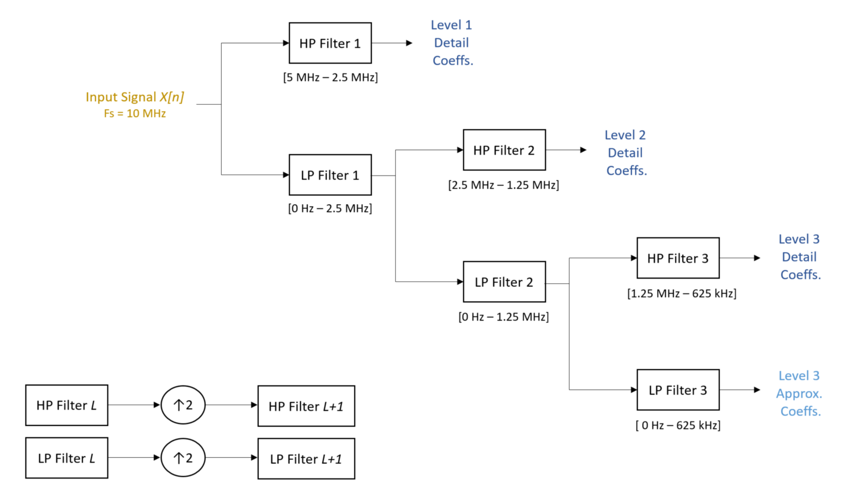
In this paper, we are focused on the application of the Wavelet Transform (WT), and, in particular, the Stationary Wavelet Transform (SWT). This tool allows for the decomposition of the measured signals in frequency bands, which can retrieve significant information about the fault given the close relationship between the propagation of TW across the system and their frequency content. The arrival of the wave-front of the TW is accurately detected using Dynamic Mode Decomposition (DMD) [4]. This paper aims to address the main factors that need to be considered in TW-based protection for distribution systems. The main contributions of this paper can be summarized as:

• Designing a robust signal-processing treatment that facilitates a data-based interpretation of the different factors that could affect the TW propagation in the first 50 $\mathsf{\mu }$s after the fault detection; and, in particular, that allows us to estimate the TW’s energy in several frequency bands between 100 kHz and 5 MHz;
• Providing insights about how fault signatures on distribution systems vary due to distance, fault types, and the presence of elements such as capacitor banks, regulators, laterals, and extra branches inside protection. This analysis is performed attending to the TW energy variations created by such elements and factors. Suggestions for suitable capacitor banks and regulators modeling for high-frequency studies are provided as well.

The rest of the paper is structured as follows: Section 2 summarizes state-of-the art approaches for using TWs for power system protection applications. Section 3 explains the signal-processing tools that are used in this work. Next, Section 4 describes the designed distribution system and the fault simulation process. Section 5 shows the results of the factor analysis corresponding to the faults’ energy signatures. Finally, Section 6 contains the conclusions for this work.

2. Background

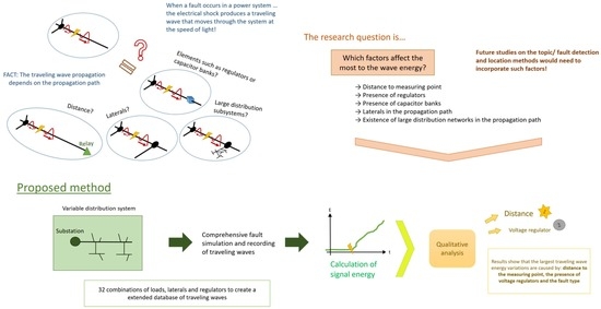
When a fault occurs in a power system (i.e., when the conductors get in contact between themselves or with a conductive ground, with the subsequent depression of voltage and a dangerous increase in current), the sudden movement of charges creates a series of high-frequency oscillations that propagates across the system at a speed close to light [5,6,7,8]. These oscillations are known as Traveling Waves (TW).

What makes TWs especially attractive for their application in distribution systems is the same fact that makes them so difficult to use: the TW, as it moves away from the fault location, is attenuated and distorted. The main reasons behind attenuation are losses due to line impedance and propagation through system elements or across junctions. Distortion is mainly caused by differences in the propagation of frequency components through the lines (TW spectrum ranges from some Hz or kHz up to MHz, and the line parameters are no longer constant for such a wide range, leading to heterogeneous propagation velocities). In addition, reflections when crossing a junction or a system element modify the shape of the TW, which causes even more distortion [5,9]. Eventually, the frequency components that can be measured in a TW are closely related to the propagation path.

The idea of using TWs is not new at the transmission level. There are multiple works that use them [1]. Some approaches decompose the incoming TW into independent modes and then calculate the TW energy to retrieve the propagation direction [10]. In the market, there exist commercial relays based on TW analysis technology for transmission lines that integrate the measured signals, after filtering out the lower frequencies, to calculate the signal energy and detect an incoming TW [11,12]. Based on the TW reflections, they are able to retrieve the fault location in both single-ended and double-ended schemes [13]. Other works use, for example, the time difference between reflections to estimate the distance to the fault [14,15], while others prefer to decompose the TW signals into independent modes and use the time difference between the several modes’ arrival times instead [16].

However, given that there are multiple factors that affect the TW propagation, the idea of determining which are the most relevant arises. This has become especially necessary for developing TW-based fault location methods that are not useful just for one system, but that can be instead generalized to other systems that may not have a similar configuration. Most of the research methods that have been developed for TWs are for transmission lines, but distribution systems are more complex, and the number of potential reflections increases exponentially. Therefore, methods that may work at the transmission level are not suitable for transmission systems. In addition, distributions systems are more dynamic than their transmission counterparts: varying loads and new connections (especially if there are distributed energy resources involved) creates a changing environment for TW propagation.

Such fast but delicate phenomena require advanced signal-processing tools to extract the information. A reliable TW arrival detection needs sensitive methods. In this reference [11], it is explained how relays are triggered after a certain increase in the measured energy is detected. In reference [4], the Dynamic Mode Decomposition (DMD) is the selected approach to find anomalies in the measured signal, which could indicate the presence of a fault. The amount of energy contained in the high-frequency components of the signal can also indicate the arrival of a TW [17]. Finally, Machine-Learning (ML) methods can be trained to detect incipient faults [18].

As indicated by several references [5,19], the measured three-phase signals can be decomposed into independent modes. Each mode has different propagation velocities and attenuation coefficients. Aerial modes propagate faster than the ground mode, although the latest shows a greater effect of attenuation. This is why the information in the ground mode is chosen by many to perform the fault location task. In addition, there are methods that take advantage of the differences in the arrival times to calculate the fault location [16].

There are also multiple approaches for extracting the information in the TW. A widespread option is to decompose the signals by frequency bands applying WTs and to study them independently. This method has been successfully used for event characterization, fault classification, and fault location [2,17,18,20,21,22,23]. This method is especially suitable for studying TWs as the fault signatures, and its frequency components are heavily influenced by the fault location and the propagation path. However, it is not the only option. Other methods that do not study the frequency spectrum directly, such as Mathematical Morphology (MM), or even DMD, can be applied [1]. Successful results can be obtained for those two even in the presence of noise [3,24]. Note that fault location approaches in distribution systems mainly depend on ML techniques due to the complexity of the measured TWs [25,26,27,28]. The work in [2] is the first paper that proposes a fault location method for just 50 $\mathsf{\mu }$s of fault data after the TW detection.

However, although there are exceptional references that theoretically explain the TW phenomena in detail [5,6,7,8], their findings are not easily extrapolated to simulated or even real data. Other works use TW to perform fault location, but there is a lack of research that aims to explain why these data are suitable for this task, and how the employed system (and their elements) affects the TW propagation. By studying the TWs’ frequency characteristics, this paper aims to provide insights toward the TW propagation under the presence of several system elements in the first microseconds after the TW fault detection.

3. Materials and Methods

Figure 1 shows the workflow of the proposed method. As an overview, the description and the tools employed for each of the main steps can be summarized as follows. The next sections will provide more details about each of the steps.

• Fault detection: Uses DMD in [4] to find the TW arrival time;
• Signal processing and feature creation: Decomposes the signal in decoupled modes Karrenbauer Transform (KT), then decomposes the signal in frequency bands using the SWT, and calculates the energy per band using the Parseval’s Energy (PE) theorem.

3.1. Fault Detection

The same implementation as in [4] was used for fault detection. The algorithm was fed with the 3-phase voltage measurements. Internally, the method performs a Singular Value Decomposition (SVD) of the measurements and an eigenvalue decomposition. The algorithm works over a window of time and summarizes the behavior of the system in a pair of eigenvalues. If there is any sudden perturbation in the measurements, the eigenvalues become significantly larger. Using a sliding window allowed us to monitor the magnitude of those eigenvalues and obtain the accurate timestamp of the TW arrival. Once the fault is detected, the signal is cropped ±50 $\mathsf{\mu }$s before and after that timestamp.

3.2. Signal Processing

3.2.1. Karrenbauer Transform

Once the measurements are taken, both 3-phase voltages and currents were transformed into three independent modes using the KT. For voltages, the operation was as follows:

$$\left[\begin{array}{c}{V}_0\\ V_{\alpha }\\ V_{\beta }\end{array}\right]=\frac{1}{3}\left[\begin{array}{ccc}1& 1& 1\\ -1& 0& 1\\ 0& -1& 1\end{array}\right]\left[\begin{array}{c}{V}_a\\ V_b\\ V_c\end{array}\right],$$

(1)

where $V_a$, $V_b$, and $V_c$ are the three-phase voltage signals, and $V_0$, $V_{\alpha }$, and $V_{\beta }$ are, respectively, the ground mode and the two aerial modes. For the analysis of the distance and system elements effect, only the ground mode was employed. The main reason was to keep explanations simple and to reduce the number of figures. In addition, using the ground mode provides an advantage from a data analysis point of view: the pre-fault measurements (and the associated energy) should be close to zero prior to the fault inception, unless the system is significantly unbalanced. Therefore, any change in voltage or current due to fault conditions is magnified. However, for the analysis of the fault type as a factor, all decomposition modes become relevant.

3.2.2. Stationary Wavelet Transform

The SWT was used to decompose the fault signals into several frequency bands to allow for a more individualized analysis per frequency component. The SWT was preferred over other WTs for two reasons: First, discrete wavelet transforms, in general, are implemented more efficiently than the Continuous Wavelet Transform (CWT), returning a result faster. Second, the SWT is preferred over the default Discrete Wavelet Transform (DWT) because it is shift-invariant. The DWT downsamples the data during the decomposition process, so the actual coefficients depend on the position of the samples. If the signal is shifted in time, the result will be different. This is avoided using the SWT.

The SWT decomposition works by passing the signal through a series of high-pass and low-pass half-band filters organized in several levels. The outputs of the high-pass filter are called “detail coefficients”. The outputs of the low-pass filter are the “approximation coefficients” and are fed into the next level of decomposition. This structure, which can be appreciated in Figure 2, is similar to sub-band filtering. As mentioned before, the key difference with the DWT is that, instead of downsampling the signal by 2 in each level and keeping the filter length constant, the length of the signal is kept constant while the length of the filters is upsampled by 2. Following this approach, all of the detail coefficients have the same length in the SWT.

The filters are obtained from a mother wavelet. In this work, Daubechies 10 was the wavelet used for decomposition. Daubechies is a family of signals that are commonly employed in the study of fast-transients because their sharp shape is suitable for detecting low amplitude, short duration, and fast decay signals [29]. The wavelet of order 10 was chosen because it provides a good balance between the sharpness of their cut-off frequencies and computational complexity [30]. The signals were decomposed into 6 frequency bands. The filters were updated by inserting zeroes between the filter coefficients. In order to recursively reduce the cut-off frequency by 2 in each decomposition level, the number of zeroes was increased exponentially. The ranges of the frequency bands for the 6 decomposition levels are shown in

Table 1. SWT Boundaries for frequency bands.

Decomposition Level	Lower Frequency	Upper Frequency
1	2.5 MHz	5 MHz
2	1.25 MHz	2.5 MHz
3	625 kHz	1.25 MHz
4	312.5 kHz	625 kHz
5	156.25 kHz	312.5 kHz
6	78.125 kHz	156.25 kHz

.

It is important to note that the detail coefficients were reconstructed back using the inverse process. This way, a set of signals in voltage and current signals were obtained back. Each of the signals represent the measurements in a certain frequency range, achieving the desired signal decomposition.

3.2.3. Parseval’s Energy Theorem

Once the signals were decomposed into frequency bands, the energy of each band was calculated using the PE theorem. For a discrete signal, the energy over a finite period of time is calculated as:

$$E=\sum _{n=1}^N{\left|x\left[n\right]\right|}^2,$$

(2)

where N is the total number of samples. From a purely data analytics point of view, the PE theorem gives a convenient way of inferring the strength of the signal. After the TW arrival, the measured signal could jump either into a more positive or a more negative value. This would mainly depend on the polarity of the measured waveforms. However, this does not mean that a negative jump has less energy than a positive jump of the same size [31]. For both fault scenarios, we were interested only in the inherent frequency components and on the time-evolution of the signal magnitude, but not on the actual sign of the measured voltages and currents. Then, squaring the waveform values takes the sign discussion out of the equation (if necessary, polarity can be added later as another feature). In addition, squaring the signals has a positive side-effect, which is that any jump in the signal will be amplified. This is desirable, as any sudden change in the TW (which is the effect of discontinuities in the system) or differences in magnitude (due to attenuation produced by the lines or other system elements) will be even more obvious.

Note that we calculated the energy for each frequency band. The application of the PE theorem in our method implies that, as we first conducted a signal decomposition before applying the theorem, what we were really performing was measuring the energy contained in each frequency band and how it varies over time. The interpretation of the energy of the signal as a monotonically increasing and time-varying function provides valuable information about the fault conditions. Different fault types, locations, and propagation paths will create different energy signatures.

4. The Use Case

4.1. The System

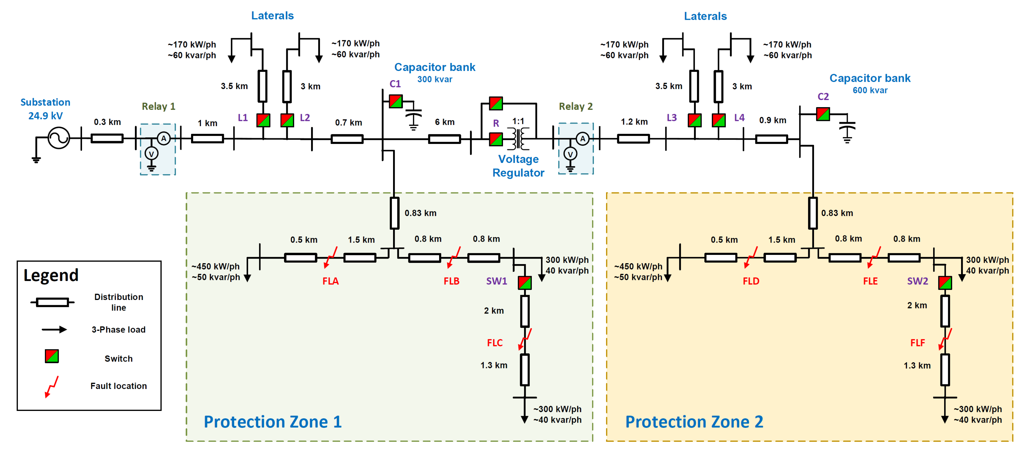
The system used in this paper is shown in Figure 3. We use a simplified representation of a distribution system that is composed of two Protection Zones (PZs). The second zone could be considered as the equivalent system of a larger network. The zones are named Protection Zone 1 (PZ1) and Protection Zone 2 (PZ2). The motivation for using this simplified system is to facilitate the observation of the individual elements’ effect on the TW propagation.

Measurements are taken on two protection devices: Relay 1 (R1) and Relay 2 (R2). The first relay is located at the terminals of the substation in order to have a general view of the distribution system. The second device is located between the two protection zones and aims to serve the second protection zone. These devices measure both the voltage and current at a sampling frequency of 10 MHz. It is worth noting that the relays are considered to be directional relays and only trigger when a fault is located downstream. This means that R1 can detect faults in both PZ1 and PZ2, but R2 works only for faults in PZ2.

In order to resemble a realistic system, faults are simulated under several load scenarios and element participation configurations. Regarding the first one, the amount of load is controlled by the connection of three-phase laterals modeled by a medium-length distribution line with an unbalanced load at the end. In addition, both protection zones are equipped with a switch that can be activated to allow for the connection of an extra branch. Adding these extra lines also modifies the propagation path and the number of measured reflections. Regarding other system elements, each protection zone has a capacitor bank in order to modify the amount of drawn reactive power. In addition, one voltage regulator is located between the two zones. This regulator can be bypassed in order to not consider its presence in the TW propagation path. In addition, note that all of the loads in the system are slightly asymmetrical.

It is important to note that the capacitor bank model includes the Equivalent Series Inductance (ESL), in order to provide a more accurate frequency response. This parasitic impedance is negligible at 60 Hz, but becomes significant at higher frequencies, and therefore it cannot be obviated [32,33]. In addition, a fixed inductor is also placed in series to avoid large currents flowing into the bank. The value of these inductances can add up to a few hundreds of microhenries for distribution level systems [34]. Both inductances become especially relevant for the capacitor bank frequency response for fast transients. In this work, the total value used, accounting for both inductances, is 200 $\mathsf{\mu }$H.

Similarly, the voltage regulator is also adapted to high-frequency transient studies. The frequency-dependent modeling of a transformer is complex because the wiring, geometrical structure, and any peculiarity/alteration on those elements has an effect on the frequency response [35]. The new reflection and refraction coefficients would depend on both the transformer impedance and the equivalent impedance on the secondary side [36].Therefore, different transformer models have to be used depending on the desired frequency range of study [37]. For high frequencies (especially over 100 kHz), the response is mainly dominated by the stray capacitance. A similar conclusion is reached in [38,39]. In industry, it is a standard to consider the stray capacitance when a high-frequency characterization of the transformer behavior is needed [9]. For these reasons, in this work, the effect of a voltage regulator between the protection zones for fast transient studies is modeled by the stray capacitance. For distribution-rated transformers, this capacitance is about a few nanofarads [40,41]. In this work, a shunt capacitance of 10 nF placed in the regulator location represents the capacitive behavior that the transformer has at frequencies above 100 kHz (which is the region of study). For the steady-state simulation, it is considered that the transfer ratio is 1:1. For the transient simulation, the action of the core (and the transfer ratio) is no longer important [37].

In order to distinguish between the effects of other elements, and to allow for a fair comparison, the two protection zones are composed of the same elements. The distribution system starts at the substation, and no faults on the main feeder are considered. Note that no faults were included on the capacitor banks, the regulator, or the laterals since they are considered as perturbations to the measurements, and not areas to protect. In total, 32 different scenarios are considered for this system. The combinations for capacitor banks, laterals, the regulator, and extra branches are shown in the next set of tables:

Table 2. Capacitor bank combinations (“1”: Connected, “0”: Not connected).

Combination	C1	C2
A	0	0
B	0	1
C	1	0
D	1	1

,

Table 3. Lateral combinations (“1”: Connected, “0”: Not connected).

Combination	L1	L2	L3	L4
A	0	0	1	0
B	0	1	0	0
C	0	1	1	0

,

Table 4. Regulator combinations (“1”: Active, “0”: Not present).

Combination	R
A	0
B	1

and

Table 5. Protection Zone Extra Branch Combinations (“1”: Connected, “0”: Not connected).

Combination	SW1	SW2
A	0	1
B	1	0
C	1	1

, respectively. Note that “1” means that the element is present in the system, whereas “0” means that it is not in the system. These elements can be activated/deactivated with their corresponding switches. For the regulator, the state of the bypass switch is always in the inverse state of R.

4.2. The Dataset

The total number of simulated faults is 6440. This takes into account:

• Three types of Single-Line-to-Ground (SLG) faults (phase-A-to-ground, phase-B-to-ground, and phase-C-to-ground), three types of Line-to-Line (LL) faults (phase-A-to-phase-B, phase-A-to-phase-C, and phase-B-to-phase-C), and the three-phase (3P) fault;
• Five fault resistance values between 0.01 and 10 ohms;
• Six fault locations (three in each protection zone);
• Three lateral settings, three extra branch settings, four capacitor bank settings, and two voltage regulator settings.

As mentioned before, the faults are decomposed into the ground mode and the two aerial modes for both voltage and current magnitudes. Then, each of the modes are decomposed into six frequency bands using the SWT, and the PE is calculated. This gives a total of 36 energy levels. As faults are cropped by ±50 $\mathsf{\mu }$s before and after the TW detection and the sampling frequency is 10 MHz, each of the levels have 1000 samples. Therefore, the generated dataset is a 3D matrix of size 6440-by-36-by-1000.

5. Results

This section analyzes in a qualitative manner the factors that are behind the largest differences within the generated data, which is the PE values per frequency bands. Those factors are considered as the most relevant for TW propagation on distribution systems. As introduced before, in a distribution system, there are multiple reasons that could significantly change the wave energy or that may be relevant in the wave propagation. The factors under consideration in this work are: distance, system elements that are present on the propagation path, and fault type. The following subsections analyze each of the factors independently. Note that the statistical data shown on the plots for the effect of system elements and fault type can be found in Appendix A in

Table A1. PE Values capacitor banks.

PE Level	Relay Zone	Combination	Mean	Standard Deviation	Median
Level 1	PZ1 R1	[0, 0]	1.003 × ${10}^{-08}$	2.919 × ${10}^{-08}$	8.856 × ${10}^{-12}$
		[0, 1]	1.134 × ${10}^{-08}$	3.318 × ${10}^{-08}$	2.436 × ${10}^{-12}$
		[1, 0]	9.250 × ${10}^{-09}$	2.823 × ${10}^{-08}$	2.436 × ${10}^{-12}$
		[1, 1]	1.003 × ${10}^{-08}$	3.069 × ${10}^{-08}$	2.316 × ${10}^{-12}$
	PZ2 R2	[0, 0]	2.386 × ${10}^{-09}$	1.059 × ${10}^{-08}$	2.014 × ${10}^{-13}$
		[0, 1]	2.963 × ${10}^{-09}$	1.266 × ${10}^{-08}$	2.120 × ${10}^{-13}$
		[1, 0]	3.251 × ${10}^{-09}$	1.364 × ${10}^{-08}$	1.926 × ${10}^{-13}$
		[1, 1]	2.608 × ${10}^{-09}$	1.159 × ${10}^{-08}$	1.857 × ${10}^{-13}$
	PZ2 R1	[0, 0]	6.680 × ${10}^{-13}$	5.798 × ${10}^{-12}$	2.207 × ${10}^{-16}$
		[0, 1]	3.470 × ${10}^{-14}$	1.037 × ${10}^{-13}$	1.208 × ${10}^{-16}$
		[1, 0]	4.428 × ${10}^{-14}$	1.159 × ${10}^{-13}$	2.682 × ${10}^{-16}$
		[1, 1]	3.284 × ${10}^{-14}$	9.391 × ${10}^{-14}$	1.665 × ${10}^{-16}$
Level 2	PZ1 R1	[0, 0]	2.043 × ${10}^{-05}$	5.473 × ${10}^{-05}$	5.110 × ${10}^{-08}$
		[0, 1]	2.306 × ${10}^{-05}$	6.197 × ${10}^{-05}$	4.561 × ${10}^{-08}$
		[1, 0]	1.883 × ${10}^{-05}$	5.291 × ${10}^{-05}$	4.346 × ${10}^{-08}$
		[1, 1]	2.043 × ${10}^{-05}$	5.752 × ${10}^{-05}$	4.185 × ${10}^{-08}$
	PZ2 R2	[0, 0]	6.760 × ${10}^{-06}$	2.768 × ${10}^{-05}$	2.892 × ${10}^{-09}$
		[0, 1]	8.276 × ${10}^{-06}$	3.255 × ${10}^{-05}$	2.933 × ${10}^{-09}$
		[1, 0]	9.177 × ${10}^{-06}$	3.546 × ${10}^{-05}$	3.055 × ${10}^{-09}$
		[1, 1]	7.316 × ${10}^{-06}$	3.002 × ${10}^{-05}$	2.819 × ${10}^{-09}$
	PZ2 R1	[0, 0]	1.088 × ${10}^{-09}$	3.656 × ${10}^{-09}$	2.392 × ${10}^{-11}$
		[0, 1]	7.812 × ${10}^{-10}$	2.178 × ${10}^{-09}$	1.475 × ${10}^{-11}$
		[1, 0]	9.993 × ${10}^{-10}$	2.445 × ${10}^{-09}$	2.485 × ${10}^{-11}$
		[1, 1]	7.520 × ${10}^{-10}$	1.957 × ${10}^{-09}$	2.108 × ${10}^{-11}$
Level 3	PZ1 R1	[0, 0]	2.599 × ${10}^{-03}$	6.275 × ${10}^{-03}$	1.502 × ${10}^{-05}$
		[0, 1]	2.935 × ${10}^{-03}$	7.111 × ${10}^{-03}$	1.416 × ${10}^{-05}$
		[1, 0]	2.377 × ${10}^{-03}$	6.011 × ${10}^{-03}$	1.276 × ${10}^{-05}$
		[1, 1]	2.570 × ${10}^{-03}$	6.515 × ${10}^{-03}$	1.262 × ${10}^{-05}$
	PZ2 R2	[0, 0]	1.532 × ${10}^{-03}$	5.585 × ${10}^{-03}$	2.355 × ${10}^{-06}$
		[0, 1]	1.791 × ${10}^{-03}$	6.285 × ${10}^{-03}$	2.332 × ${10}^{-06}$
		[1, 0]	2.080 × ${10}^{-03}$	7.178 × ${10}^{-03}$	3.177 × ${10}^{-06}$
		[1, 1]	1.583 × ${10}^{-03}$	5.777 × ${10}^{-03}$	2.266 × ${10}^{-06}$
	PZ2 R1	[0, 0]	5.704 × ${10}^{-07}$	1.230 × ${10}^{-06}$	5.677 × ${10}^{-08}$
		[0, 1]	5.157 × ${10}^{-07}$	1.206 × ${10}^{-06}$	4.558 × ${10}^{-08}$
		[1, 0]	6.624 × ${10}^{-07}$	1.404 × ${10}^{-06}$	6.374 × ${10}^{-08}$
		[1, 1]	5.013 × ${10}^{-07}$	1.119 × ${10}^{-06}$	5.537 × ${10}^{-08}$
Level 4	PZ1 R1	[0, 0]	1.698 × ${10}^{-01}$	3.662 × ${10}^{-01}$	1.592 × ${10}^{-03}$
		[0, 1]	1.890 × ${10}^{-01}$	4.088 × ${10}^{-01}$	1.570 × ${10}^{-03}$
		[1, 0]	1.440 × ${10}^{-01}$	3.220 × ${10}^{-01}$	1.293 × ${10}^{-03}$
		[1, 1]	1.546 × ${10}^{-01}$	3.466 × ${10}^{-01}$	1.291 × ${10}^{-03}$
	PZ2 R2	[0, 0]	5.341 × ${10}^{-02}$	1.758 × ${10}^{-01}$	3.178 × ${10}^{-04}$
		[0, 1]	4.968 × ${10}^{-02}$	1.578 × ${10}^{-01}$	2.362 × ${10}^{-04}$
		[1, 0]	7.058 × ${10}^{-02}$	2.207 × ${10}^{-01}$	3.552 × ${10}^{-04}$
		[1, 1]	4.450 × ${10}^{-02}$	1.461 × ${10}^{-01}$	2.286 × ${10}^{-04}$
	PZ2 R1	[0, 0]	2.011 × ${10}^{-04}$	4.384 × ${10}^{-04}$	2.528 × ${10}^{-05}$
		[0, 1]	1.855 × ${10}^{-04}$	3.865 × ${10}^{-04}$	2.414 × ${10}^{-05}$
		[1, 0]	2.291 × ${10}^{-04}$	4.721 × ${10}^{-04}$	3.005 × ${10}^{-05}$
		[1, 1]	1.587 × ${10}^{-04}$	3.255 × ${10}^{-04}$	2.274 × ${10}^{-05}$
Level 5	PZ1 R1	[0, 0]	3.770 × ${10}^{-01}$	7.370 × ${10}^{-01}$	3.580 × ${10}^{-03}$
		[0, 1]	4.087 × ${10}^{-01}$	8.069 × ${10}^{-01}$	3.601 × ${10}^{-03}$
		[1, 0]	3.264 × ${10}^{-01}$	6.778 × ${10}^{-01}$	2.538 × ${10}^{-03}$
		[1, 1]	3.424 × ${10}^{-01}$	7.135 × ${10}^{-01}$	2.560 × ${10}^{-03}$
	PZ2 R2	[0, 0]	6.224 × ${10}^{-01}$	1.810 × ${10}^{+00}$	5.266 × ${10}^{-03}$
		[0, 1]	3.345 × ${10}^{-01}$	9.641 × ${10}^{-01}$	3.118 × ${10}^{-03}$
		[1, 0]	8.087 × ${10}^{-01}$	2.248 × ${10}^{+00}$	6.538 × ${10}^{-03}$
		[1, 1]	3.053 × ${10}^{-01}$	9.089 × ${10}^{-01}$	3.112 × ${10}^{-03}$
	PZ2 R1	[0, 0]	4.684 × ${10}^{-03}$	1.268 × ${10}^{-02}$	3.121 × ${10}^{-04}$
		[0, 1]	3.343 × ${10}^{-03}$	9.029 × ${10}^{-03}$	2.613 × ${10}^{-04}$
		[1, 0]	4.789 × ${10}^{-03}$	1.236 × ${10}^{-02}$	3.395 × ${10}^{-04}$
		[1, 1]	2.561 × ${10}^{-03}$	7.438 × ${10}^{-03}$	2.204 × ${10}^{-04}$
Level 6	PZ1 R1	[0, 0]	5.418 × ${10}^{+00}$	1.192 × ${10}^{+01}$	8.885 × ${10}^{-02}$
		[0, 1]	6.557 × ${10}^{+00}$	1.474 × ${10}^{+01}$	8.547 × ${10}^{-02}$
		[1, 0]	2.237 × ${10}^{+00}$	5.947 × ${10}^{+00}$	6.922 × ${10}^{-02}$
		[1, 1]	2.635 × ${10}^{+00}$	6.773 × ${10}^{+00}$	6.842 × ${10}^{-02}$
	PZ2 R2	[0, 0]	2.957 × ${10}^{+00}$	7.337 × ${10}^{+00}$	3.312 × ${10}^{-02}$
		[0, 1]	8.210 × ${10}^{-01}$	1.946 × ${10}^{+00}$	8.484 × ${10}^{-03}$
		[1, 0]	4.180 × ${10}^{+00}$	1.023 × ${10}^{+01}$	3.363 × ${10}^{-02}$
		[1, 1]	7.625 × ${10}^{-01}$	1.844 × ${10}^{+00}$	8.479 × ${10}^{-03}$
	PZ2 R1	[0, 0]	5.182 × ${10}^{-01}$	1.254 × ${10}^{+00}$	2.834 × ${10}^{-02}$
		[0, 1]	1.023 × ${10}^{-01}$	2.544 × ${10}^{-01}$	1.026 × ${10}^{-02}$
		[1, 0]	2.225 × ${10}^{-01}$	5.690 × ${10}^{-01}$	2.821 × ${10}^{-02}$
		[1, 1]	3.575 × ${10}^{-02}$	9.407 × ${10}^{-02}$	6.277 × ${10}^{-03}$

,

Table A2. PE values laterals.

PE Level	Relay Zone	Combination	Mean	Standard Deviation	Median
Level 1	PZ1 R1	[0, 0, 1, 0]	1.698 × ${10}^{-08}$	4.565 × ${10}^{-08}$	4.330 × ${10}^{-13}$
		[0, 1, 0, 0]	7.084 × ${10}^{-09}$	1.980 × ${10}^{-08}$	6.655 × ${10}^{-12}$
		[0, 1, 1, 0]	7.515 × ${10}^{-09}$	2.018 × ${10}^{-08}$	7.589 × ${10}^{-12}$
	PZ2 R2	[0, 0, 1, 0]	1.826 × ${10}^{-09}$	7.434 × ${10}^{-09}$	2.397 × ${10}^{-13}$
		[0, 1, 0, 0]	4.671 × ${10}^{-09}$	1.788 × ${10}^{-08}$	7.562 × ${10}^{-14}$
		[0, 1, 1, 0]	1.815 × ${10}^{-09}$	7.389 × ${10}^{-09}$	3.727 × ${10}^{-18}$
	PZ2 R1	[0, 0, 1, 0]	9.756 × ${10}^{-17}$	2.169 × ${10}^{-16}$	3.727 × ${10}^{-18}$
		[0, 1, 0, 0]	5.517 × ${10}^{-13}$	5.026 × ${10}^{-12}$	1.199 × ${10}^{-15}$
		[0, 1, 1, 0]	3.043 × ${10}^{-14}$	6.357 × ${10}^{-14}$	4.893 × ${10}^{-16}$
Level 2	PZ1 R1	[0, 0, 1, 0]	3.459 × ${10}^{-05}$	8.534 × ${10}^{-05}$	2.277 × ${10}^{-08}$
		[0, 1, 0, 0]	1.441 × ${10}^{-05}$	3.698 × ${10}^{-05}$	4.839 × ${10}^{-08}$
		[0, 1, 1, 0]	1.527 × ${10}^{-05}$	3.760 × ${10}^{-05}$	5.010 × ${10}^{-08}$
	PZ2 R2	[0, 0, 1, 0]	5.147 × ${10}^{-06}$	1.933 × ${10}^{-05}$	2.917 × ${10}^{-09}$
		[0, 1, 0, 0]	1.311 × ${10}^{-05}$	4.622 × ${10}^{-05}$	2.229 × ${10}^{-09}$
		[0, 1, 1, 0]	5.125 × ${10}^{-06}$	1.925 × ${10}^{-05}$	2.894 × ${10}^{-09}$
	PZ2 R1	[0, 0, 1, 0]	2.087 × ${10}^{-11}$	4.337 × ${10}^{-11}$	1.676 × ${10}^{-12}$
		[0, 1, 0, 0]	1.918 × ${10}^{-09}$	4.115 × ${10}^{-09}$	7.004 × ${10}^{-11}$
		[0, 1, 1, 0]	7.160 × ${10}^{-10}$	1.373 × ${10}^{-09}$	3.258 × ${10}^{-11}$
Level 3	PZ1 R1	[0, 0, 1, 0]	4.323 × ${10}^{-03}$	9.638 × ${10}^{-03}$	8.592 × ${10}^{-06}$
		[0, 1, 0, 0]	1.856 × ${10}^{-03}$	4.313 × ${10}^{-03}$	1.378 × ${10}^{-05}$
		[0, 1, 1, 0]	1.957 × ${10}^{-03}$	4.358 × ${10}^{-03}$	1.402 × ${10}^{-05}$
	PZ2 R2	[0, 0, 1, 0]	1.139 × ${10}^{-03}$	3.810 × ${10}^{-03}$	2.052 × ${10}^{-06}$
		[0, 1, 0, 0]	2.897 × ${10}^{-03}$	9.108 × ${10}^{-03}$	4.266 × ${10}^{-06}$
		[0, 1, 1, 0]	1.143 × ${10}^{-03}$	3.825 × ${10}^{-03}$	2.053 × ${10}^{-06}$
	PZ2 R1	[0, 0, 1, 0]	8.485 × ${10}^{-08}$	1.850 × ${10}^{-07}$	7.986 × ${10}^{-09}$
		[0, 1, 0, 0]	1.101 × ${10}^{-06}$	1.826 × ${10}^{-06}$	1.500 × ${10}^{-07}$
		[0, 1, 1, 0]	4.649 × ${10}^{-07}$	7.993 × ${10}^{-07}$	5.978 × ${10}^{-08}$
Level 4	PZ1 R1	[0, 0, 1, 0]	2.636 × ${10}^{-01}$	5.279 × ${10}^{-01}$	1.128 × ${10}^{-03}$
		[0, 1, 0, 0]	1.204 × ${10}^{-01}$	2.524 × ${10}^{-01}$	1.542 × ${10}^{-03}$
		[0, 1, 1, 0]	1.267 × ${10}^{-01}$	2.555 × ${10}^{-01}$	1.547 × ${10}^{-03}$
	PZ2 R2	[0, 0, 1, 0]	3.506 × ${10}^{-02}$	1.062 × ${10}^{-01}$	2.298 × ${10}^{-04}$
		[0, 1, 0, 0]	8.969 × ${10}^{-02}$	2.580 × ${10}^{-01}$	3.724 × ${10}^{-04}$
		[0, 1, 1, 0]	3.682 × ${10}^{-02}$	1.117 × ${10}^{-01}$	2.675 × ${10}^{-04}$
	PZ2 R1	[0, 0, 1, 0]	1.318 × ${10}^{-04}$	3.800 × ${10}^{-04}$	4.355 × ${10}^{-06}$
		[0, 1, 0, 0]	3.070 × ${10}^{-04}$	5.285 × ${10}^{-04}$	5.274 × ${10}^{-05}$
		[0, 1, 1, 0]	1.380 × ${10}^{-04}$	2.428 × ${10}^{-04}$	2.315 × ${10}^{-05}$
Level 5	PZ1 R1	[0, 0, 1, 0]	5.255 × ${10}^{-01}$	1.004 × ${10}^{+00}$	3.461 × ${10}^{-03}$
		[0, 1, 0, 0]	2.920 × ${10}^{-01}$	5.746 × ${10}^{-01}$	2.753 × ${10}^{-03}$
		[0, 1, 1, 0]	3.040 × ${10}^{-01}$	5.782 × ${10}^{-01}$	3.035 × ${10}^{-03}$
	PZ2 R2	[0, 0, 1, 0]	3.130 × ${10}^{-01}$	9.184 × ${10}^{-01}$	3.218 × ${10}^{-03}$
		[0, 1, 0, 0]	8.514 × ${10}^{-01}$	2.311 × ${10}^{+00}$	6.562 × ${10}^{-03}$
		[0, 1, 1, 0]	3.652 × ${10}^{-01}$	1.046 × ${10}^{+00}$	3.621 × ${10}^{-03}$
	PZ2 R1	[0, 0, 1, 0]	3.550 × ${10}^{-03}$	9.823 × ${10}^{-03}$	1.308 × ${10}^{-04}$
		[0, 1, 0, 0]	5.488 × ${10}^{-03}$	1.389 × ${10}^{-02}$	2.561 × ${10}^{-04}$
		[0, 1, 1, 0]	2.512× ${10}^{-03}$	6.733× ${10}^{-03}$	2.561× ${10}^{-04}$
Level 6	PZ1 R1	[0, 0, 1, 0]	9.190 × ${10}^{+00}$	1.780 × ${10}^{+01}$	8.056 × ${10}^{-02}$
		[0, 1, 0, 0]	2.142 × ${10}^{+00}$	4.433 × ${10}^{+00}$	7.389 × ${10}^{-02}$
		[0, 1, 1, 0]	2.481 × ${10}^{+00}$	4.994 × ${10}^{+00}$	7.840 × ${10}^{-02}$
	PZ2 R2	[0, 0, 1, 0]	1.263 × ${10}^{+00}$	3.434 × ${10}^{+00}$	1.824 × ${10}^{-02}$
		[0, 1, 0, 0]	3.574 × ${10}^{+00}$	9.708 × ${10}^{+00}$	2.875 × ${10}^{-02}$
		[0, 1, 1, 0]	1.579 × ${10}^{+00}$	4.024 × ${10}^{+00}$	2.007 × ${10}^{-02}$
	PZ2 R1	[0, 0, 1, 0]	3.207 × ${10}^{-01}$	1.013 × ${10}^{+00}$	4.443 × ${10}^{-03}$
		[0, 1, 0, 0]	2.220 × ${10}^{-01}$	6.603 × ${10}^{-01}$	2.455 × ${10}^{-02}$
		[0, 1, 1, 0]	1.579 × ${10}^{+00}$	4.024 × ${10}^{+00}$	2.007 × ${10}^{-02}$

,

Table A3. PE values regulator.

PE Level	Relay Zone	Combination	Mean	Standard Deviation	Median
Level 1	PZ1 R1	[0]	1.023 × ${10}^{-08}$	3.052 × ${10}^{-08}$	2.868 × ${10}^{-12}$
		[1]	1.023 × ${10}^{-08}$	3.052 × ${10}^{-08}$	2.868 × ${10}^{-12}$
	PZ2 R2	[0]	5.621 × ${10}^{-09}$	1.679 × ${10}^{-08}$	6.988 × ${10}^{-13}$
		[1]	2.665 × ${10}^{-12}$	7.919 × ${10}^{-12}$	4.276 × ${10}^{-16}$
	PZ2 R1	[0]	2.384 × ${10}^{-13}$	2.991 × ${10}^{-12}$	6.675 × ${10}^{-15}$
		[1]	1.653 × ${10}^{-13}$	2.959 × ${10}^{-12}$	1.415 × ${10}^{-17}$
Level 2	PZ1 R1	[0]	2.081 × ${10}^{-05}$	5.714 × ${10}^{-05}$	4.512 × ${10}^{-08}$
		[1]	2.081 × ${10}^{-05}$	5.714 × ${10}^{-05}$	4.513 × ${10}^{-08}$
	PZ2 R2	[0]	1.578 × ${10}^{-05}$	4.332 × ${10}^{-05}$	1.292 × ${10}^{-08}$
		[1]	3.259 × ${10}^{-08}$	8.885 × ${10}^{-08}$	3.172 × ${10}^{-11}$
	PZ2 R1	[0]	1.714 × ${10}^{-09}$	3.230 × ${10}^{-09}$	1.854 × ${10}^{-10}$
		[1]	1.008 × ${10}^{-10}$	1.588 × ${10}^{-09}$	1.600 × ${10}^{-12}$
Level 3	PZ1 R1	[0]	2.637 × ${10}^{-03}$	6.525 × ${10}^{-03}$	1.369 × ${10}^{-05}$
		[1]	2.638 × ${10}^{-03}$	6.525 × ${10}^{-03}$	1.369 × ${10}^{-05}$
	PZ2 R2	[0]	3.478 × ${10}^{-03}$	8.494 × ${10}^{-03}$	9.513 × ${10}^{-06}$
		[1]	2.539 × ${10}^{-05}$	6.197 × ${10}^{-05}$	8.741 × ${10}^{-08}$
	PZ2 R1	[0]	1.086 × ${10}^{-06}$	1.591 × ${10}^{-06}$	2.648 × ${10}^{-07}$
		[1]	3.875 × ${10}^{-08}$	1.887 × ${10}^{-07}$	5.769 × ${10}^{-09}$
Level 4	PZ1 R1	[0]	1.659 × ${10}^{-01}$	3.657 × ${10}^{-01}$	1.507 × ${10}^{-03}$
		[1]	1.659 × ${10}^{-01}$	3.658 × ${10}^{-01}$	1.507 × ${10}^{-03}$
	PZ2 R2	[0]	1.067 × ${10}^{-01}$	2.401 × ${10}^{-01}$	6.329 × ${10}^{-04}$
		[1]	2.596 × ${10}^{-03}$	5.870 × ${10}^{-03}$	1.881 × ${10}^{-05}$
	PZ2 R1	[0]	3.725 × ${10}^{-04}$	5.260 × ${10}^{-04}$	1.802 × ${10}^{-04}$
		[1]	1.700 × ${10}^{-05}$	2.294 × ${10}^{-05}$	7.818 × ${10}^{-06}$
Level 5	PZ1 R1	[0]	3.655 × ${10}^{-01}$	7.381 × ${10}^{-01}$	3.014 × ${10}^{-03}$
		[1]	3.679 × ${10}^{-01}$	7.433 × ${10}^{-01}$	3.012 × ${10}^{-03}$
	PZ2 R2	[0]	9.547 × ${10}^{-01}$	2.164 × ${10}^{+00}$	6.967 × ${10}^{-03}$
		[1]	7.987 × ${10}^{-02}$	1.849 × ${10}^{-01}$	8.073 × ${10}^{-04}$
	PZ2 R1	[0]	7.054 × ${10}^{-03}$	1.441 × ${10}^{-02}$	5.343 × ${10}^{-04}$
		[1]	7.171 × ${10}^{-04}$	1.443 × ${10}^{-03}$	1.499 × ${10}^{-04}$
Level 6	PZ1 R1	[0]	4.369 × ${10}^{+00}$	1.097 × ${10}^{+01}$	7.747 × ${10}^{-02}$
		[1]	4.412 × ${10}^{+00}$	1.110 × ${10}^{+01}$	7.792 × ${10}^{-02}$
	PZ2 R2	[0]	3.444 × ${10}^{+00}$	8.800 × ${10}^{+00}$	3.337 × ${10}^{-02}$
		[1]	8.963 × ${10}^{-01}$	2.294 × ${10}^{+00}$	9.387 × ${10}^{-03}$
	PZ2 R1	[0]	3.501 × ${10}^{-01}$	9.849 × ${10}^{-01}$	2.449 × ${10}^{-02}$
		[1]	1.030 × ${10}^{-01}$	2.922 × ${10}^{-01}$	1.001 × ${10}^{-02}$

,

Table A4. PE values extra branch on protection zone.

PE Level	Relay Zone	Combination	Mean	Standard Deviation	Median
Level 1	PZ1 R1	[0, 1]	1.700 × ${10}^{-08}$	4.070 × ${10}^{-08}$	6.053 × ${10}^{-11}$
		[1, 0]	7.120 × ${10}^{-09}$	1.990 × ${10}^{-08}$	6.739 × ${10}^{-12}$
		[1, 1]	9.990 × ${10}^{-09}$	3.060 × ${10}^{-08}$	2.477 × ${10}^{-12}$
	PZ2 R2	[0, 1]	1.830 × ${10}^{-09}$	7.440 × ${10}^{-09}$	2.377 × ${10}^{-13}$
		[1, 0]	6.270 × ${10}^{-09}$	2.050 × ${10}^{-08}$	3.993 × ${10}^{-13}$
		[1, 1]	2.590 × ${10}^{-09}$	1.150 × ${10}^{-08}$	1.877 × ${10}^{-13}$
	PZ2 R1	[0, 1]	1.550 × ${10}^{-14}$	4.810 × ${10}^{-14}$	5.787 × ${10}^{-17}$
		[1, 0]	9.540 × ${10}^{-14}$	1.750 × ${10}^{-13}$	1.260 × ${10}^{-15}$
		[1, 1]	2.450 × ${10}^{-13}$	3.360 × ${10}^{-12}$	1.656 × ${10}^{-16}$
Level 2	PZ1 R1	[0, 1]	3.440 × ${10}^{-05}$	7.520 × ${10}^{-05}$	6.483 × ${10}^{-08}$
		[1, 0]	1.450 × ${10}^{-05}$	3.720 × ${10}^{-05}$	4.873 × ${10}^{-08}$
		[1, 1]	2.040 × ${10}^{-05}$	5.730 × ${10}^{-05}$	4.341 × ${10}^{-08}$
	PZ2 R2	[0, 1]	5.160 × ${10}^{-06}$	1.940 × ${10}^{-05}$	2.934 × ${10}^{-09}$
		[1, 0]	1.750 × ${10}^{-05}$	5.240 × ${10}^{-05}$	8.948 × ${10}^{-09}$
		[1, 1]	7.310 × ${10}^{-06}$	3.000 × ${10}^{-05}$	2.837 × ${10}^{-09}$
	PZ2 R1	[0, 1]	3.800 × ${10}^{-10}$	1.070 × ${10}^{-09}$	1.085 × ${10}^{-11}$
		[1, 0]	2.070 × ${10}^{-09}$	3.690 × ${10}^{-09}$	7.597 × ${10}^{-11}$
		[1, 1]	8.660 × ${10}^{-10}$	2.680 × ${10}^{-09}$	2.098 × ${10}^{-11}$
Level 3	PZ1 R1	[0, 1]	4.310 × ${10}^{-03}$	8.530 × ${10}^{-03}$	1.559 × ${10}^{-05}$
		[1, 0]	1.860 × ${10}^{-03}$	4.330 × ${10}^{-03}$	1.395 × ${10}^{-05}$
		[1, 1]	2.580 × ${10}^{-03}$	6.540 × ${10}^{-03}$	1.352 × ${10}^{-05}$
	PZ2 R2	[0, 1]	1.150 × ${10}^{-03}$	3.830 × ${10}^{-03}$	2.048 × ${10}^{-06}$
		[1, 0]	3.860 × ${10}^{-03}$	1.040 × ${10}^{-02}$	1.044 × ${10}^{-05}$
		[1, 1]	1.620 × ${10}^{-03}$	5.910 × ${10}^{-03}$	2.303 × ${10}^{-06}$
	PZ2 R1	[0, 1]	2.800 × ${10}^{-07}$	6.310 × ${10}^{-07}$	2.561 × ${10}^{-08}$
		[1, 0]	1.220 × ${10}^{-06}$	1.950 × ${10}^{-06}$	1.678 × ${10}^{-07}$
		[1, 1]	5.360 × ${10}^{-07}$	1.200 × ${10}^{-06}$	5.590 × ${10}^{-08}$
Level 4	PZ1 R1	[0, 1]	2.660 × ${10}^{-01}$	4.780 × ${10}^{-01}$	1.804 × ${10}^{-03}$
		[1, 0]	1.210 × ${10}^{-01}$	2.540 × ${10}^{-01}$	1.563 × ${10}^{-03}$
		[1, 1]	1.620 × ${10}^{-01}$	3.650 × ${10}^{-01}$	1.403 × ${10}^{-03}$
	PZ2 R2	[0, 1]	3.610 × ${10}^{-02}$	1.090 × ${10}^{-01}$	2.477 × ${10}^{-04}$
		[1, 0]	1.150 × ${10}^{-01}$	2.860 × ${10}^{-01}$	6.329 × ${10}^{-04}$
		[1, 1]	5.110 × ${10}^{-02}$	1.700 × ${10}^{-01}$	2.685 × ${10}^{-04}$
	PZ2 R1	[0, 1]	1.370 × ${10}^{-04}$	3.090 × ${10}^{-04}$	1.699 × ${10}^{-05}$
		[1, 0]	3.610 × ${10}^{-04}$	5.580 × ${10}^{-04}$	6.092 × ${10}^{-05}$
		[1, 1]	1.860 × ${10}^{-04}$	4.040 × ${10}^{-04}$	2.379 × ${10}^{-05}$
Level 5	PZ1 R1	[0, 1]	5.500 × ${10}^{-01}$	9.300 × ${10}^{-01}$	4.336 × ${10}^{-03}$
		[1, 0]	2.930 × ${10}^{-01}$	5.770 × ${10}^{-01}$	2.748 × ${10}^{-03}$
		[1, 1]	3.590 × ${10}^{-01}$	7.380 × ${10}^{-01}$	2.800 × ${10}^{-03}$
	PZ2 R2	[0, 1]	3.390 × ${10}^{-01}$	9.850 × ${10}^{-01}$	3.411 × ${10}^{-03}$
		[1, 0]	1.040 × ${10}^{+00}$	2.490 × ${10}^{+00}$	7.918 × ${10}^{-03}$
		[1, 1]	4.890 × ${10}^{-01}$	1.540 × ${10}^{+00}$	3.645 × ${10}^{-03}$
	PZ2 R1	[0, 1]	3.220 × ${10}^{-03}$	8.510 × ${10}^{-03}$	2.477 × ${10}^{-04}$
		[1, 0]	6.550 × ${10}^{-03}$	1.440 × ${10}^{-02}$	6.079 × ${10}^{-04}$
		[1, 1]	3.700 × ${10}^{-03}$	1.050 × ${10}^{-02}$	2.687 × ${10}^{-04}$
Level 6	PZ1 R1	[0, 1]	1.020 × ${10}^{+01}$	1.930 × ${10}^{+01}$	9.144 × ${10}^{-02}$
		[1, 0]	2.150 × ${10}^{+00}$	4.460 × ${10}^{+00}$	7.434 × ${10}^{-02}$
		[1, 1]	4.120 × ${10}^{+00}$	1.030 × ${10}^{+01}$	7.324 × ${10}^{-02}$
	PZ2 R2	[0, 1]	1.420 × ${10}^{+00}$	3.730 × ${10}^{+00}$	1.948 × ${10}^{-02}$
		[1, 0]	4.770 × ${10}^{+00}$	1.190 × ${10}^{+01}$	2.728 × ${10}^{-02}$
		[1, 1]	2.010 × ${10}^{+00}$	6.000 × ${10}^{+00}$	2.178 × ${10}^{-02}$
	PZ2 R1	[0, 1]	2.080 × ${10}^{-01}$	4.800 × ${10}^{-01}$	1.577 × ${10}^{-02}$
		[1, 0]	1.810 × ${10}^{-01}$	3.380 × ${10}^{-01}$	3.642 × ${10}^{-02}$
		[1, 1]	2.350 × ${10}^{-01}$	8.020 × ${10}^{-01}$	1.343 × ${10}^{-02}$

,

Table A5. PE values ground mode.

PE Level	Relay Zone	Fault Type	Mean	Standard Deviation	Median
Level 1	PZ1 R1	SLG	2.385 × ${10}^{-08}$	4.300 × ${10}^{-08}$	5.819 × ${10}^{-09}$
		LL	8.515 × ${10}^{-12}$	1.791 × ${10}^{-11}$	4.565 × ${10}^{-13}$
		3P	1.557 × ${10}^{-11}$	2.433 × ${10}^{-11}$	1.466 × ${10}^{-12}$
	PZ2 R2	SLG	6.560 × ${10}^{-09}$	1.797 × ${10}^{-08}$	4.765 × ${10}^{-12}$
		LL	4.309 × ${10}^{-13}$	4.534 × ${10}^{-12}$	2.525 × ${10}^{-16}$
		3P	8.456 × ${10}^{-14}$	1.510 × ${10}^{-13}$	5.427 × ${10}^{-16}$
	PZ2 R1	SLG	1.185 × ${10}^{-14}$	3.497 × ${10}^{-14}$	5.741 × ${10}^{-17}$
		LL	4.309 × ${10}^{-13}$	4.534 × ${10}^{-12}$	2.525 × ${10}^{-16}$
		3P	8.456 × ${10}^{-14}$	1.510 × ${10}^{-13}$	5.427 × ${10}^{-16}$
Level 2	PZ1 R1	SLG	4.853 × ${10}^{-05}$	7.921 × ${10}^{-05}$	1.570 × ${10}^{-05}$
		LL	1.841 × ${10}^{-08}$	2.041 × ${10}^{-08}$	6.518 × ${10}^{-09}$
		3P	3.559 × ${10}^{-08}$	2.745 × ${10}^{-08}$	2.293 × ${10}^{-08}$
	PZ2 R2	SLG	1.845 × ${10}^{-05}$	4.626 × ${10}^{-05}$	1.050 × ${10}^{-07}$
		LL	2.921 × ${10}^{-09}$	6.499 × ${10}^{-09}$	7.410 × ${10}^{-11}$
		3P	3.801 × ${10}^{-09}$	5.400 × ${10}^{-09}$	7.765 × ${10}^{-10}$
	PZ2 R1	SLG	2.665 × ${10}^{-10}$	7.200 × ${10}^{-10}$	1.132 × ${10}^{-11}$
		LL	1.208 × ${10}^{-09}$	3.453 × ${10}^{-09}$	2.251 × ${10}^{-11}$
		3P	1.929 × ${10}^{-09}$	3.166 × ${10}^{-09}$	6.712 × ${10}^{-11}$
Level 3	PZ1 R1	SLG	6.146 × ${10}^{-03}$	8.821 × ${10}^{-03}$	2.381 × ${10}^{-03}$
		LL	5.077 × ${10}^{-06}$	5.077 × ${10}^{-06}$	3.452 × ${10}^{-06}$
		3P	9.894 × ${10}^{-06}$	5.733 × ${10}^{-06}$	8.652 × ${10}^{-06}$
	PZ2 R2	SLG	4.085 × ${10}^{-03}$	9.034 × ${10}^{-03}$	1.422 × ${10}^{-04}$
		LL	2.024 × ${10}^{-06}$	4.396 × ${10}^{-06}$	1.697 × ${10}^{-07}$
		3P	1.231 × ${10}^{-06}$	1.874 × ${10}^{-06}$	1.483 × ${10}^{-07}$
	PZ2 R1	SLG	2.665 × ${10}^{-07}$	5.609 × ${10}^{-07}$	3.270 × ${10}^{-08}$
		LL	6.349 × ${10}^{-07}$	1.381 × ${10}^{-06}$	5.768 × ${10}^{-08}$
		3P	1.231 × ${10}^{-06}$	1.874 × ${10}^{-06}$	1.483 × ${10}^{-07}$
Level 4	PZ1 R1	SLG	3.862 × ${10}^{-01}$	4.767 × ${10}^{-01}$	1.741 × ${10}^{-01}$
		LL	5.906 × ${10}^{-04}$	5.620 × ${10}^{-04}$	4.605 × ${10}^{-04}$
		3P	1.182 × ${10}^{-03}$	6.348 × ${10}^{-04}$	1.151 × ${10}^{-03}$
	PZ2 R2	SLG	1.273 × ${10}^{-01}$	2.537 × ${10}^{-01}$	1.565 × ${10}^{-02}$
		LL	1.251 × ${10}^{-04}$	2.517 × ${10}^{-04}$	2.399 × ${10}^{-05}$
		3P	1.689 × ${10}^{-04}$	2.071 × ${10}^{-04}$	6.223 × ${10}^{-05}$
	PZ2 R1	SLG	2.979 × ${10}^{-04}$	5.683 × ${10}^{-04}$	4.164 × ${10}^{-05}$
		LL	9.219 × ${10}^{-05}$	1.733 × ${10}^{-04}$	1.192 × ${10}^{-05}$
		3P	1.932 × ${10}^{-04}$	2.626 × ${10}^{-04}$	3.809 × ${10}^{-05}$
Level 5	PZ1 R1	SLG	8.540 × ${10}^{-01}$	9.298 × ${10}^{-01}$	4.640 × ${10}^{-01}$
		LL	1.079 × ${10}^{-03}$	1.318 × ${10}^{-03}$	6.383 × ${10}^{-04}$
		3P	1.854 × ${10}^{-03}$	9.941 × ${10}^{-04}$	1.463 × ${10}^{-03}$
	PZ2 R2	SLG	1.204 × ${10}^{+00}$	2.264 × ${10}^{+00}$	3.117 × ${10}^{-01}$
		LL	1.782 × ${10}^{-03}$	3.346 × ${10}^{-03}$	5.139 × ${10}^{-04}$
		3P	2.358 × ${10}^{-03}$	3.040 × ${10}^{-03}$	1.194 × ${10}^{-03}$
	PZ2 R1	SLG	8.835 × ${10}^{-03}$	1.500 × ${10}^{-02}$	2.694 × ${10}^{-03}$
		LL	1.439 × ${10}^{-04}$	1.845 × ${10}^{-04}$	7.016 × ${10}^{-05}$
		3P	2.624 × ${10}^{-04}$	2.425 × ${10}^{-04}$	1.800 × ${10}^{-04}$
Level 6	PZ1 R1	SLG	1.020 × ${10}^{+01}$	1.500 × ${10}^{+01}$	5.256 × ${10}^{+00}$
		LL	2.722 × ${10}^{-02}$	3.144 × ${10}^{-02}$	1.632 × ${10}^{-02}$
		3P	4.875 × ${10}^{-02}$	2.961 × ${10}^{-02}$	3.779 × ${10}^{-02}$
	PZ2 R2	SLG	5.050 × ${10}^{+00}$	9.260 × ${10}^{+00}$	1.655 × ${10}^{+00}$
		LL	9.055 × ${10}^{-03}$	1.757 × ${10}^{-02}$	2.265 × ${10}^{-03}$
		3P	1.228 × ${10}^{-02}$	1.590 × ${10}^{-02}$	6.590 × ${10}^{-03}$
	PZ2 R1	SLG	5.151 × ${10}^{-01}$	1.059 × ${10}^{+00}$	1.618 × ${10}^{-01}$
		LL	8.564 × ${10}^{-03}$	1.564 × ${10}^{-02}$	2.522 × ${10}^{-03}$
		3P	1.469 × ${10}^{-02}$	1.740 × ${10}^{-02}$	8.451 × ${10}^{-03}$

,

Table A6. PE values aerial 1 mode.

PE Level	Relay Zone	Fault Type	Mean	Standard Deviation	Median
Level 1	PZ1 R1	SLG	8.554 × ${10}^{-04}$	1.249 × ${10}^{-03}$	3.245 × ${10}^{-04}$
		LL	3.146 × ${10}^{-03}$	3.253 × ${10}^{-03}$	1.868 × ${10}^{-03}$
		3P	8.125 × ${10}^{-04}$	5.945 × ${10}^{-04}$	6.604 × ${10}^{-04}$
	PZ2 R2	SLG	1.145 × ${10}^{-03}$	2.739 × ${10}^{-03}$	1.867 × ${10}^{-06}$
		LL	3.186 × ${10}^{-05}$	5.299 × ${10}^{-05}$	2.305 × ${10}^{-06}$
		3P	9.394 × ${10}^{-06}$	1.277 × ${10}^{-05}$	1.131 × ${10}^{-06}$
	PZ2 R1	SLG	8.502 × ${10}^{-06}$	1.888 × ${10}^{-05}$	2.409 × ${10}^{-08}$
		LL	3.186 × ${10}^{-05}$	5.299 × ${10}^{-05}$	2.305 × ${10}^{-06}$
		3P	9.394 × ${10}^{-06}$	1.277 × ${10}^{-05}$	1.131 × ${10}^{-06}$
Level 2	PZ1 R1	SLG	3.959 × ${10}^{-02}$	5.106 × ${10}^{-02}$	2.230 × ${10}^{-02}$
		LL	1.487 × ${10}^{-01}$	1.306 × ${10}^{-01}$	1.072 × ${10}^{-01}$
		3P	3.856 × ${10}^{-02}$	2.133 × ${10}^{-02}$	3.507 × ${10}^{-02}$
	PZ2 R2	SLG	2.608 × ${10}^{-02}$	5.589 × ${10}^{-02}$	2.263 × ${10}^{-04}$
		LL	9.854 × ${10}^{-02}$	1.570 × ${10}^{-01}$	9.592 × ${10}^{-03}$
		3P	2.905 × ${10}^{-02}$	3.752 × ${10}^{-02}$	8.392 × ${10}^{-03}$
	PZ2 R1	SLG	2.285 × ${10}^{-03}$	4.664 × ${10}^{-03}$	2.129 × ${10}^{-05}$
		LL	8.579 × ${10}^{-03}$	1.291 × ${10}^{-02}$	7.805 × ${10}^{-04}$
		3P	2.533 × ${10}^{-03}$	3.067 × ${10}^{-03}$	6.119 × ${10}^{-04}$
Level 3	PZ1 R1	SLG	1.968 × ${10}^{-01}$	2.393 × ${10}^{-01}$	1.101 × ${10}^{-01}$
		LL	7.796 × ${10}^{-01}$	6.453 × ${10}^{-01}$	6.567 × ${10}^{-01}$
		3P	2.030 × ${10}^{-01}$	9.881 × ${10}^{-02}$	1.853 × ${10}^{-01}$
	PZ2 R2	SLG	1.304 × ${10}^{-01}$	2.603 × ${10}^{-01}$	4.808 × ${10}^{-03}$
		LL	5.138 × ${10}^{-01}$	7.499 × ${10}^{-01}$	8.885 × ${10}^{-02}$
		3P	2.838 × ${10}^{-02}$	3.166 × ${10}^{-02}$	9.748 × ${10}^{-03}$
	PZ2 R1	SLG	2.571 × ${10}^{-02}$	4.960 × ${10}^{-02}$	8.880 × ${10}^{-04}$
		LL	9.582 × ${10}^{-02}$	1.347 × ${10}^{-01}$	1.379 × ${10}^{-02}$
		3P	2.838 × ${10}^{-02}$	3.166 × ${10}^{-02}$	9.748 × ${10}^{-03}$
Level 4	PZ1 R1	SLG	9.558 × ${10}^{-01}$	1.117 × ${10}^{+00}$	5.503 × ${10}^{-01}$
		LL	4.382 × ${10}^{+00}$	3.366 × ${10}^{+00}$	3.750 × ${10}^{+00}$
		3P	1.165 × ${10}^{+00}$	4.810 × ${10}^{-01}$	1.161 × ${10}^{+00}$
	PZ2 R2	SLG	3.802 × ${10}^{-01}$	6.990 × ${10}^{-01}$	5.767 × ${10}^{-02}$
		LL	1.561 × ${10}^{+00}$	2.072 × ${10}^{+00}$	5.987 × ${10}^{-01}$
		3P	4.617 × ${10}^{-01}$	4.828 × ${10}^{-01}$	2.590 × ${10}^{-01}$
	PZ2 R1	SLG	1.762 × ${10}^{-01}$	3.175 × ${10}^{-01}$	2.120 × ${10}^{-02}$
		LL	7.753 × ${10}^{-01}$	1.033 × ${10}^{+00}$	2.681 × ${10}^{-01}$
		3P	2.298 × ${10}^{-01}$	2.427 × ${10}^{-01}$	1.078 × ${10}^{-01}$
Level 5	PZ1 R1	SLG	7.661 × ${10}^{-01}$	1.008 × ${10}^{+00}$	3.984 × ${10}^{-01}$
		LL	4.570 × ${10}^{+00}$	4.412 × ${10}^{+00}$	2.695 × ${10}^{+00}$
		3P	1.175 × ${10}^{+00}$	7.635 × ${10}^{-01}$	1.040 × ${10}^{+00}$
	PZ2 R2	SLG	1.028 × ${10}^{+00}$	1.672 × ${10}^{+00}$	3.477 × ${10}^{-01}$
		LL	4.490 × ${10}^{+00}$	5.023 × ${10}^{+00}$	2.402 × ${10}^{+00}$
		3P	1.302 × ${10}^{+00}$	1.098 × ${10}^{+00}$	9.768 × ${10}^{-01}$
	PZ2 R1	SLG	1.097 × ${10}^{-01}$	1.761 × ${10}^{-01}$	3.953 × ${10}^{-02}$
		LL	5.052 × ${10}^{-01}$	5.527 × ${10}^{-01}$	2.945 × ${10}^{-01}$
		3P	1.444 × ${10}^{-01}$	1.159 × ${10}^{-01}$	1.108 × ${10}^{-01}$
Level 6	PZ1 R1	SLG	2.508 × ${10}^{+00}$	3.536 × ${10}^{+00}$	1.104 × ${10}^{+00}$
		LL	1.082 × ${10}^{+01}$	1.262 × ${10}^{+01}$	6.746 × ${10}^{+00}$
		3P	2.880 × ${10}^{+00}$	2.404 × ${10}^{+00}$	1.896 × ${10}^{+00}$
	PZ2 R2	SLG	1.899 × ${10}^{+00}$	2.766 × ${10}^{+00}$	7.628 × ${10}^{-01}$
		LL	8.329 × ${10}^{+00}$	8.995 × ${10}^{+00}$	5.519 × ${10}^{+00}$
		3P	2.428 × ${10}^{+00}$	1.878 × ${10}^{+00}$	1.811 × ${10}^{+00}$
	PZ2 R1	SLG	1.015 × ${10}^{+00}$	1.583 × ${10}^{+00}$	4.302 × ${10}^{-01}$
		LL	4.674 × ${10}^{+00}$	5.945 × ${10}^{+00}$	2.650 × ${10}^{+00}$
		3P	1.396 × ${10}^{+00}$	1.360 × ${10}^{+00}$	9.016 × ${10}^{-01}$

and

Table A7. PE values aerial 2 mode.

PE Level	Relay Zone	Fault Type	Mean	Standard Deviation	Median
Level 1	PZ1 R1	SLG	2.233 × ${10}^{-03}$	2.896 × ${10}^{-03}$	7.396 × ${10}^{-04}$
		LL	8.191 × ${10}^{-03}$	1.289 × ${10}^{-02}$	2.709 × ${10}^{-03}$
		3P	2.113 × ${10}^{-02}$	1.565 × ${10}^{-02}$	1.678 × ${10}^{-02}$
	PZ2 R2	SLG	2.982 × ${10}^{-03}$	6.350 × ${10}^{-03}$	5.497 × ${10}^{-06}$
		LL	8.259 × ${10}^{-05}$	1.929 × ${10}^{-04}$	1.074 × ${10}^{-06}$
		3P	2.137 × ${10}^{-04}$	2.917 × ${10}^{-04}$	2.652 × ${10}^{-05}$
	PZ2 R1	SLG	2.214 × ${10}^{-05}$	4.357 × ${10}^{-05}$	7.646 × ${10}^{-08}$
		LL	8.259 × ${10}^{-05}$	1.929 × ${10}^{-04}$	1.074 × ${10}^{-06}$
		3P	2.137 × ${10}^{-04}$	2.917 × ${10}^{-04}$	2.652 × ${10}^{-05}$
Level 2	PZ1 R1	SLG	1.037 × ${10}^{-01}$	1.171 × ${10}^{-01}$	7.198 × ${10}^{-02}$
		LL	3.881 × ${10}^{-0}$	5.439 × ${10}^{-01}$	1.455 × ${10}^{-01}$
		3P	1.001 × ${10}^{+00}$	5.671 × ${10}^{-01}$	8.994 × ${10}^{-01}$
	PZ2 R2	SLG	6.780 × ${10}^{-02}$	1.289 × ${10}^{-01}$	8.965 × ${10}^{-04}$
		LL	2.552 × ${10}^{-01}$	5.747 × ${10}^{-01}$	9.486 × ${10}^{-03}$
		3P	6.610 × ${10}^{-01}$	8.590 × ${10}^{-01}$	1.975 × ${10}^{-01}$
	PZ2 R1	SLG	5.968 × ${10}^{-03}$	1.076 × ${10}^{-02}$	8.240 × ${10}^{-05}$
		LL	2.231 × ${10}^{-02}$	4.779 × ${10}^{-02}$	8.404 × ${10}^{-04}$
		3P	5.777 × ${10}^{-02}$	7.025 × ${10}^{-02}$	1.441 × ${10}^{-02}$
Level 3	PZ1 R1	SLG	5.163 × ${10}^{-01}$	5.448 × ${10}^{-01}$	4.232 × ${10}^{-01}$
		LL	2.041 × ${10}^{+00}$	2.748 × ${10}^{+00}$	7.729 × ${10}^{-01}$
		3P	5.267 × ${10}^{+00}$	2.656 × ${10}^{+00}$	4.794 × ${10}^{+00}$
	PZ2 R2	SLG	3.383 × ${10}^{-01}$	5.967 × ${10}^{-01}$	1.921 × ${10}^{-02}$
		LL	1.329 × ${10}^{+00}$	2.781 × ${10}^{+00}$	1.001 × ${10}^{-01}$
		3P	6.466 × ${10}^{-01}$	7.241 × ${10}^{-01}$	2.277 × ${10}^{-01}$
	PZ2 R1	SLG	6.723 × ${10}^{-02}$	1.142 × ${10}^{-01}$	3.555 × ${10}^{-03}$
		LL	2.496 × ${10}^{-01}$	5.043 × ${10}^{-01}$	1.864 × ${10}^{-02}$
		3P	6.466 × ${10}^{-01}$	7.241 × ${10}^{-01}$	2.277 × ${10}^{-01}$
Level 4	PZ1 R1	SLG	2.519 × ${10}^{+00}$	2.541 × ${10}^{+00}$	2.162 × ${10}^{+00}$
		LL	1.155 × ${10}^{+01}$	1.486 × ${10}^{+01}$	4.739 × ${10}^{+00}$
		3P	2.985 × ${10}^{+01}$	1.276 × ${10}^{+01}$	2.962 × ${10}^{+01}$
	PZ2 R2	SLG	9.855 × ${10}^{-01}$	1.595 × ${10}^{+00}$	1.871 × ${10}^{-01}$
		LL	4.039 × ${10}^{+00}$	7.814 × ${10}^{+00}$	5.617 × ${10}^{-01}$
		3P	1.046 × ${10}^{+01}$	1.097 × ${10}^{+01}$	5.781 × ${10}^{+00}$
	PZ2 R1	SLG	4.635 × ${10}^{-01}$	7.368 × ${10}^{-01}$	8.187 × ${10}^{-02}$
		LL	2.040 × ${10}^{+00}$	3.970 × ${10}^{+00}$	2.344 × ${10}^{-01}$
		3P	5.290 × ${10}^{+00}$	5.608 × ${10}^{+00}$	2.475 × ${10}^{+00}$
Level 5	PZ1 R1	SLG	2.012 × ${10}^{+00}$	2.342 × ${10}^{+00}$	1.302 × ${10}^{+00}$
		LL	1.196 × ${10}^{+01}$	1.793 × ${10}^{+01}$	4.274 × ${10}^{+00}$
		3P	3.108 × ${10}^{+01}$	2.077 × ${10}^{+01}$	2.649 × ${10}^{+01}$
	PZ2 R2	SLG	2.665 × ${10}^{+00}$	3.788 × ${10}^{+00}$	1.124 × ${10}^{+00}$
		LL	1.163 × ${10}^{+01}$	1.970 × ${10}^{+01}$	3.485 × ${10}^{+00}$
		3P	3.014 × ${10}^{+01}$	2.549 × ${10}^{+01}$	2.245 × ${10}^{+01}$
	PZ2 R1	SLG	2.859 × ${10}^{-01}$	4.011 × ${10}^{-01}$	1.322 × ${10}^{-01}$
		LL	1.313 × ${10}^{+00}$	2.188 × ${10}^{+00}$	4.134 × ${10}^{-01}$
		3P	3.410 × ${10}^{+00}$	2.810 × ${10}^{+00}$	2.618 × ${10}^{+00}$
Level 6	PZ1 R1	SLG	6.653 × ${10}^{+00}$	8.241 × ${10}^{+00}$	4.465 × ${10}^{+00}$
		LL	2.853 × ${10}^{+01}$	4.897 × ${10}^{+01}$	7.444 × ${10}^{+00}$
		3P	7.373 × ${10}^{+01}$	6.412 × ${10}^{+01}$	4.627 × ${10}^{+01}$
	PZ2 R2	SLG	4.917 × ${10}^{+00}$	6.221 × ${10}^{+00}$	3.300 × ${10}^{+00}$
		LL	2.157 × ${10}^{+01}$	3.576 × ${10}^{+01}$	6.664 × ${10}^{+00}$
		3P	5.584 × ${10}^{+01}$	4.541 × ${10}^{+01}$	4.276 × ${10}^{+01}$
	PZ2 R1	SLG	2.688 × ${10}^{+00}$	3.617 × ${10}^{+00}$	1.499 × ${10}^{+00}$
		LL	1.235 × ${10}^{+01}$	2.308 × ${10}^{+01}$	3.162 × ${10}^{+00}$
		3P	3.205 × ${10}^{+01}$	3.192 × ${10}^{+01}$	2.131 × ${10}^{+01}$

. Due to space considerations, only the plots of voltage magnitudes are presented in this paper. In the end, voltage and current signals exhibit a similar pattern of attenuation and distortion. The most noticeable differences are in the reflection coefficients at junctions; however, a detailed explanation of this effect is beyond the scope of this paper. For distance and system elements analysis, only the ground mode is used. However, for the fault type analysis, the three independent decomposition modes are considered to provide further insights into the TW propagation.

Hereafter, the terms “PZ1 R1”, “PZ2 R2”, and “PZ2 R2” will be used. The first part of the abbreviation refers to the protection zone, where the fault occurs, whereas the second is related to the relay, where the measurements are captured.

5.1. Distance

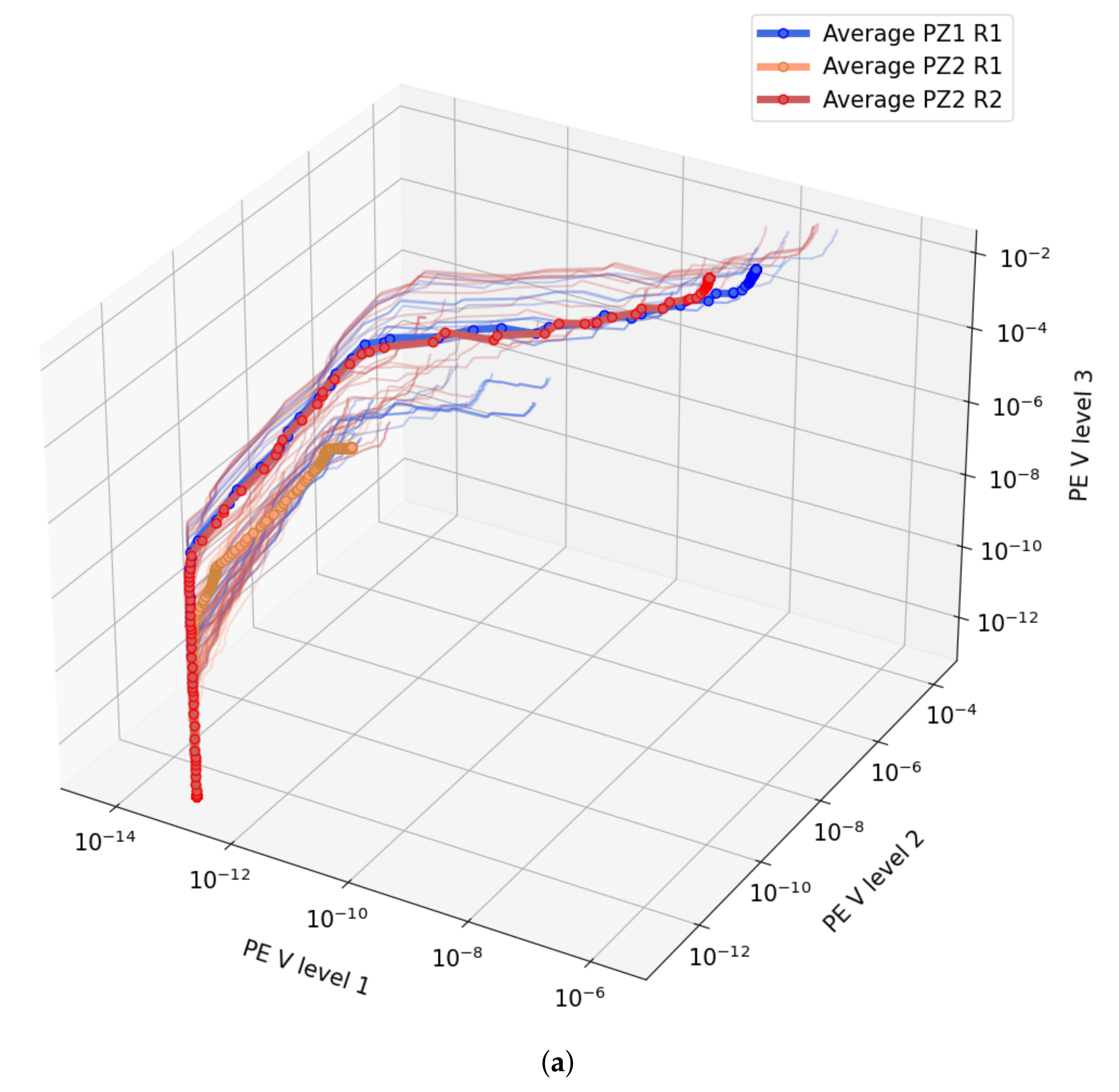
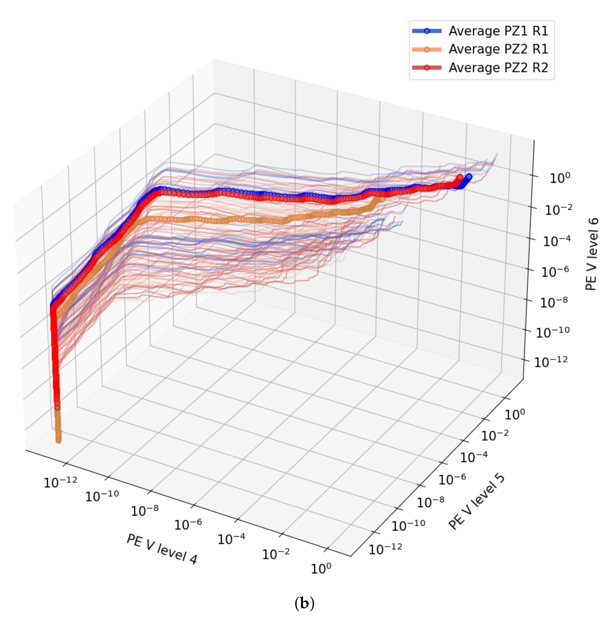
Figure 4 shows a comparison of the energy signatures that are measured from faults in both PZ1 and PZ2, as seen from Relay 1, and for faults in PZ2, as seen from Relay 2. The goal is to check if there is any difference between faults in the next protection zone (PZ1 R1 and PZ2 R2) and faults that come from farther away (PZ2 R1). As there are six energy levels in the ground mode to analyze in total, they are divided into two groups of three (Levels 1 to 3 and 4 to 6) in order to create two 3D plots that show the evolution of the fault energy and the interaction between levels. Note that all fault signature arrays are of the same length (1000 samples). The more energy contained in each PE level, the further it will reach in its particular axis. This allows us to clearly distinguish the faults with more energy. On top of the fault signatures, the average fault signatures for faults in PZ1 R1, PZ2 R2, and PZ2 R1 have been plotted using a thicker line. Note that, for plotting purposes, a common origin has been created adding an offset of magnitude ${10}^{-13}$. Therefore, all energy signatures start in the same spatial point independently of how small the first PE value is for each level.

Comparing faults in PZ1 R1 and PZ2 R1, it can be seen that the values for PZ2 R1 cases are smaller than for PZ1 R1 ones. However, for faults in PZ2 R2, both the individual traces and the average energy values are closer to faults on PZ1 R1. This means that the attenuation given by the distribution line that separates the two zones (whose length is 7 km) is enough to set a difference between the two areas. Analyzing the plots in more detail, it can be seen in Figure 4a that the energy increase for “Average PZ2 R1” is very small in comparison to both “Average PZ1 R1" and “Average PZ2 R2”. The frequency components between 625 kHz and 5 MHz have considerably shrunk several orders of magnitude due to the 7 km line between the two protection zones. However, in Figure 4b, the energy increase for “Average PZ2 R1”, although smaller in magnitude, is more similar to its counterparts in “Average PZ1 R1” and “Average PZ2 R2”. This means that attenuation is relatively less remarkable in the frequency range between 78.125 and 625 kHz.

This is an important result for TW-based protection in distribution systems: relatively shorter lines still produce a noticeable attenuation. This fact is actually related to the line topologies in distribution systems: conductors in the distribution network have a smaller cross-section, which increases the conductor resistance. A larger resistance implies more losses and more attenuation.

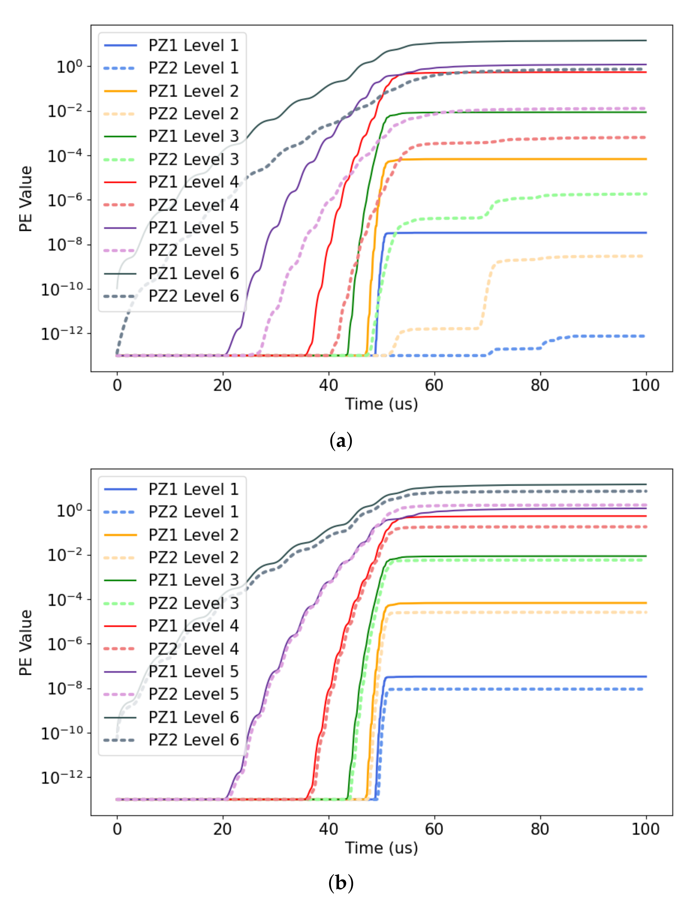
The same result can be appreciated in Figure 5. This time, average energy signatures per level for faults in PZ2 R1 and PZ2 R2 are compared against their counterparts in PZ1 R1. Average values for faults in the next protection zones are similar, whereas faults in another protection zone have comparatively lower energy in all of the levels. In this figure, it is easier to see that, after a certain number of microseconds, a “steady state” is achieved once the components are attenuated enough and are not present any more in the wave.

By the nature of the studied transients, the first decomposition level shows fast increments of energy but in a small amount of time (as those frequency components are rapidly attenuated), whereas analyzing higher levels of decomposition shows comparatively slower increments of energy that are more sustained across time. Overall, higher decomposition levels (lower frequencies) have larger energy values by the end of the study window. Regarding the actual energy traces, it is possible to see that the first levels start to increase at around 50 $\mathsf{\mu }$s. This is because the signal is cropped ±50 $\mathsf{\mu }$s before and after the TW arrival. Due to the wavelets scaling, first levels give a high-temporal resolution but a lower frequency resolution (the frequency bands for those levels are much wider), whereas subsequent decomposition levels give a finer frequency resolution (narrower frequency bands) but a low-temporal resolution (which explains why larger decomposition levels start before the 50 $\mathsf{\mu }$s label).

Figure 5 gives critical information that corroborates TW propagation theory. Comparing “PZ1 Level 5” and “PZ2 Level 5” in Figure 5a shows that the TW energy traces coming from distant faults, on average, have a relatively lower amount of oscillations, and they are smoother. These oscillations are the representation of the reflections in the measured TW. In addition, the energy increase across time is weaker, which can be observed in the gentler slopes for those faults coming from PZ2, if compared to those coming from PZ1. This is the effect of distortion and attenuation, which is still noticeable in small distribution systems, such as the one considered in this work. The same insights can be extrapolated to all of the decomposition levels, although they are more noticeable in Levels 3 to 6 (below 1.25 MHz). It is possible to appreciate some notorious steps in PZ2 Levels 1, 2, and 3 starting at 75 $\mathsf{\mu }$s. For even such a small system, it is difficult to attribute the cause, but they are probably due to reflections in the line endings at PZ2 that came out after a few microseconds.

On the contrary, in Figure 5b, the opposite insights are shown: there is a close match between the energy traces from PZ1 and PZ2, both in magnitude, slope, and energy oscillations. This is because both PZs share the same topology. However, the average values from PZ1 R1 and PZ2 R2 are not exactly overlapping. This may be explained by the fact that the measurements for the substation relay are slightly larger because more power is flowing through that line (it goes to both zones and laterals) and, therefore, the step changes are slightly more energetic.

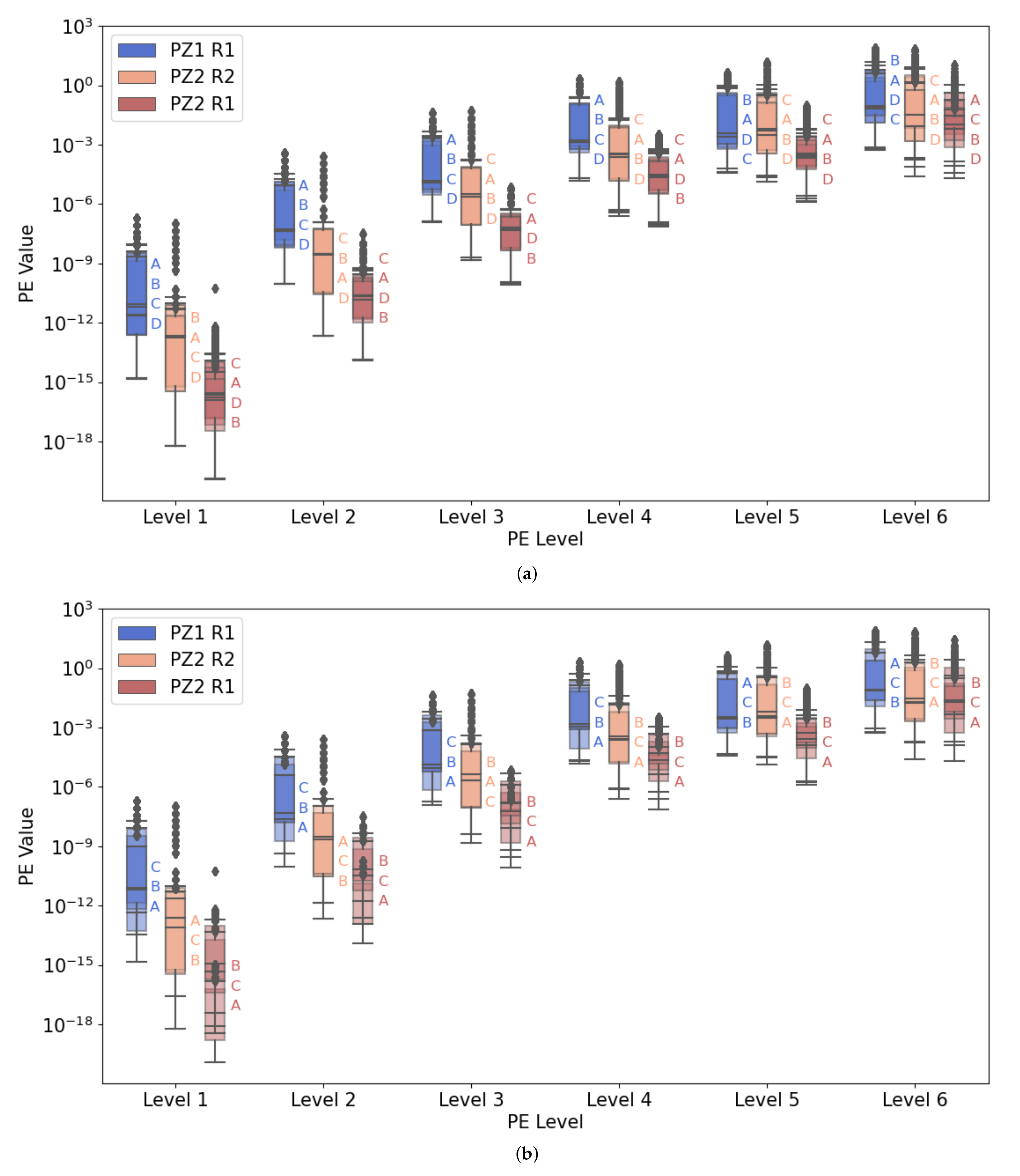
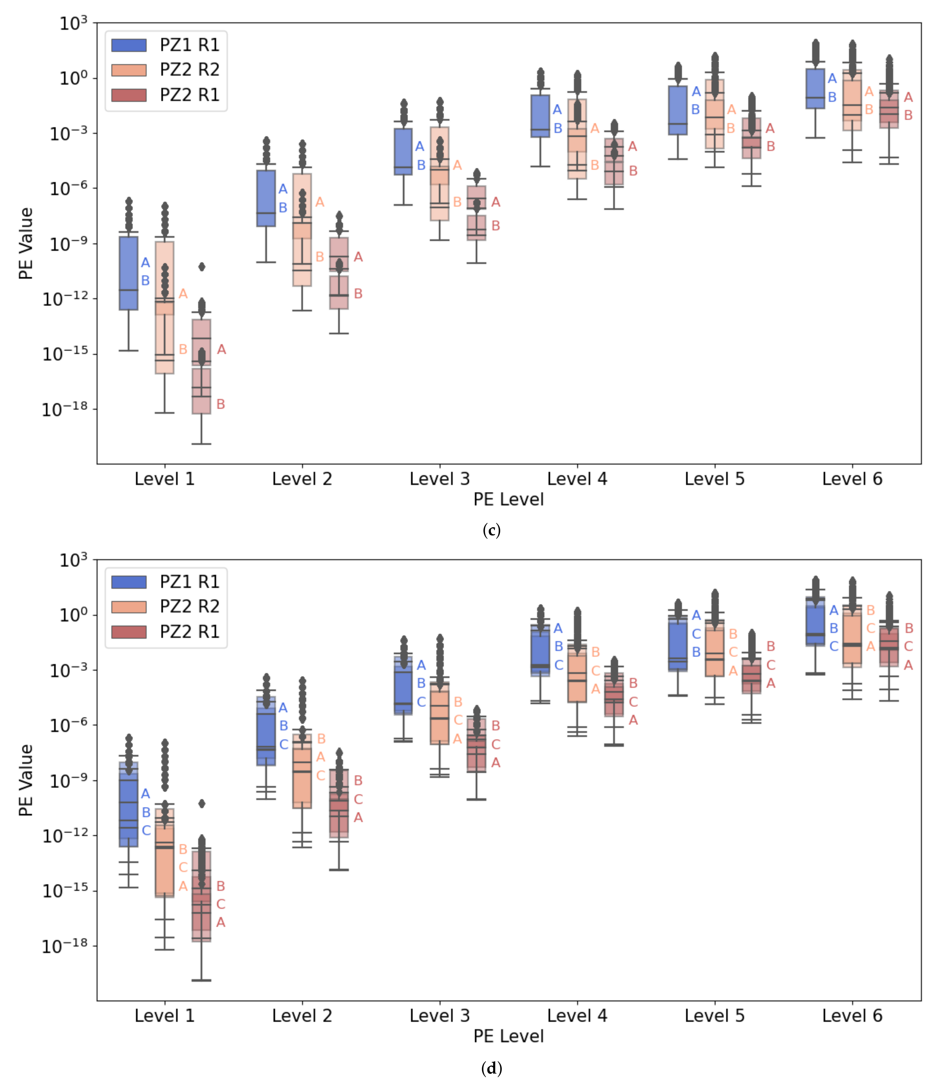
5.2. System Elements

In Figure 6, a comparison of the final PE values at the “steady-state” is organized by the type of analyzed system element (capacitor banks, regulator, laterals, or protection zone configuration). The boxes inside each protection zone are the different combinations in which the elements can be set. For example, in the capacitor banks subplot, there are four boxes per level and per PZ–relay combination because four different settings of capacitor banks participation are considered. The order of the letters on the right side indicates the relative ordering of each one of the combinations. The ordering criteria are the median of the final PE values per combinations. The meaning of the combinations per element type has been previously defined in Table 2, Table 3, Table 4 and Table 5. The median values can be observed in the Appendix A. It turns out that the main observation is still that energy values from faults on PZ2 are significantly lower than those for PZ1, for the case where both measurements correspond to R1. In general, for faults in PZ2 R2, the values are closer to the ones of faults in PZ1 R1. Therefore, energy variations due to different combinations of system elements seem to be lower than the effect of the distance between protection zones. Taking a look at the distributions, a similar conclusion as in Figure 4 and Figure 5 can be extracted from Figure 6. In conclusion, the distance to the fault (seen as the protection zone where the fault occurs) has a more significant influence than the elements that are on the propagation path.

Analyzing the different elements, it seems that the overall effect of capacitor banks is small for all of the PZ-R combinations. The largest energy variations take place on Level 6, which agrees with the frequency behavior of the capacitor banks. This is especially noticeable in PZ2 R1, which is exposed to the capacitor banks twice (note that both C1 and C2 are in the propagation path in capacitor bank combination “D”). In PZ2 R1 Level 6, the median energy value is reduced to one half when both capacitor banks are in the system, if compared to other cases. Such a significant TW energy drop is only observed in the lower frequency band (78.125 to 156.25 kHz). This is consistent with the high-frequency model of the capacitor bank: including the ESL inductance modifies the frequency response in such a way that medium-frequency components are filtered out the most.

The laterals’ and protection zones’ topologies add an extra variability to the operating conditions, which modifies the numerical voltage and current values across time (due to different initial power flow conditions) and leads to a different sequence of TW reflections. However, given the large variations in the initial drawn power (switching on all of the considered laterals and extra branches in the PZs can increase more than 50% of the base consumption), the energy values are still quite concentrated. For both types of elements, the largest variations seem to be apparent in the first decomposition levels and in Level 6. On the contrary, Levels 4 and 5 are less subject to energy variations. Analyzing Figure 6b in detail, it can be seen that the most energetic TW for PZ1 R1, looking at Levels 1 to 4, are those for lateral combination “C”, in which, the only lateral is on PZ2. In Levels 5 and 6, for PZ1 R1, a clear distinction according to the different laterals combinations cannot be made. However, for PZ2 R1, the most energetic TWs are measured for lateral combination “B”, in which, there is only one lateral in the system, and it is on PZ1. Faults in PZ2 R2 mostly follow the same trend, having more energy when the lateral is not in their PZ. This indicates that the presence of nearby laterals produces additional TW reflections and refractions that end up lowering the measured TW energy. Including extra branches and loads inside the PZs leads to similar conclusions. The more complex the nearby PZ, the lower the TW energy. This is why the most energetic faults in PZ1 R1 are for PZ combinations “A” when PZ1 is hosting fewer loads and branches. Similarly, faults in PZ2 R1 and PZ2 R2 are more energetic when PZ2 is less loaded and has fewer branches.

The only element that may draw more attention is the case of the regulator. The presence of this element in the system changes the final energy values up to a point that, for the first three levels, the PE distributions for PZ2 R1 and PZ2 R2 for regulator combinations “A” and “B” are barely overlapping. For PZ1 R1, there is no visible effect in both combinations, as the regulator is downstream. This suggests that, when the regulator is on the propagation path, the measured energy values are radically lower. The case of PZ2 R2 is of special interest: Relay 2, which is downstream from the regulator (so this element is not directly on the propagation path), still measures less energy in the case when the regulator is located upstream in combination “B”. The reason for this behavior could be that, even if the TW arrives first to Relay 2 and then to the regulator, the power is flowing downstream and goes first through the regulator. Therefore, it seems that the transients in PZ2 cannot achieve their maximum energy because the regulator is limiting the variations in power. The relative position of the PZ, at least in radial systems where the power flows downstream in just one direction, seems to be another important factor to take into account.

Another fact to observe is that the energy jumps between protection zones are larger for the first decomposition levels (highest-frequency components). In TW, attenuation is modeled with a negative exponent, which means that the effect of the attenuation factor is going to be more noticeable at the beginning of the propagation journey of the TW, rapidly decreasing the original frequency components [1]. For faults in PZ2, by the time the TW arrives at Relay 1, the highest-frequency components are practically non-existent.

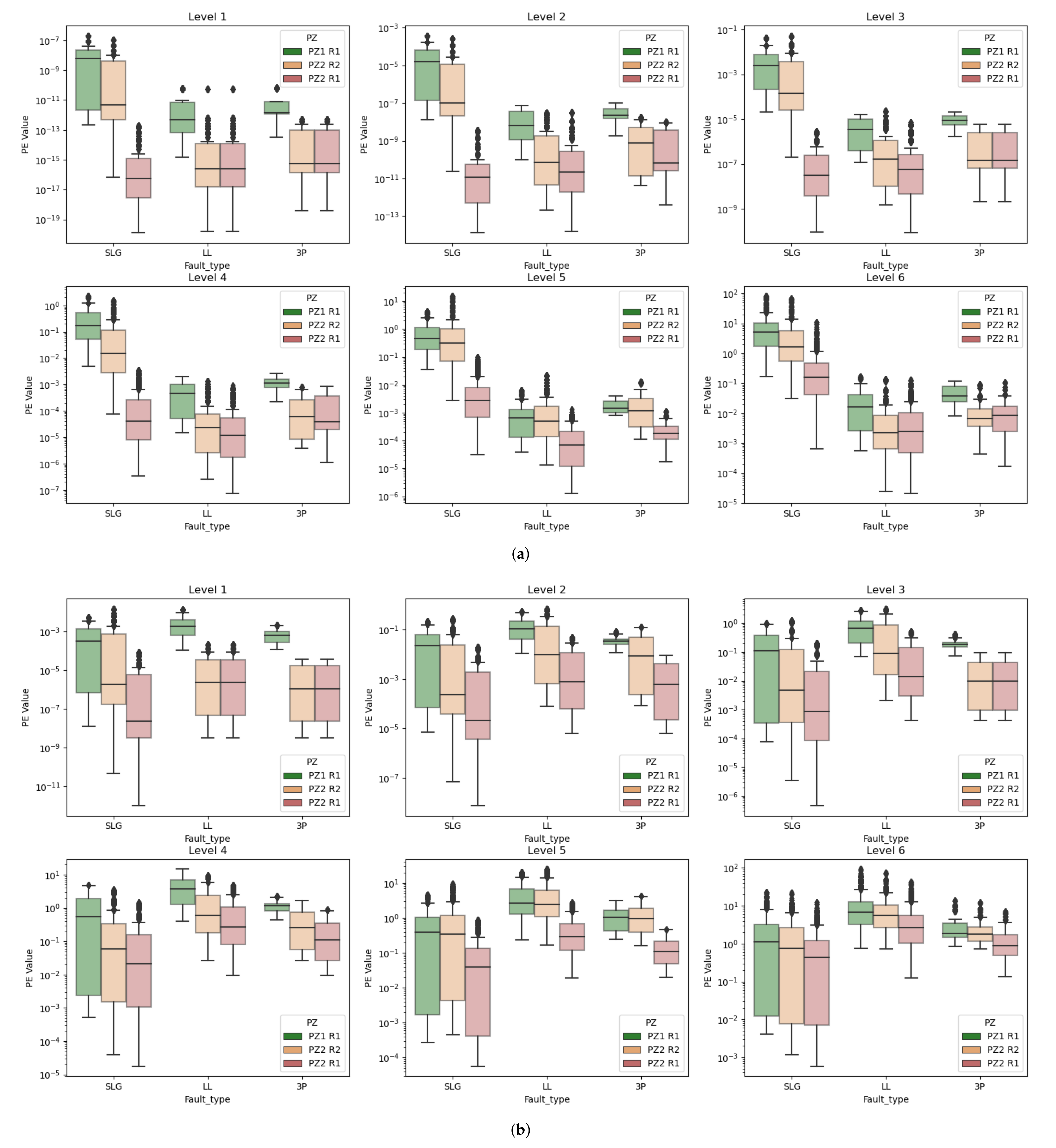
5.3. Fault Type

Figure 7 shows the same final energy value distributions as in the previous section, but, this time, the analysis is performed per level and per fault type. The ground mode and the two aerial modes are considered.

Looking at the ground mode in Figure 7a, when the fault is measured from a relay that is close to the protection zone (PZ1 R1 or PZ2 R2), the energy associated with SLG faults is, most of the time, several orders of magnitude larger than for LL or 3P faults. Note that, for every level, the energy for SLG faults for PZ1 R1 and PZ2 R2 are larger than those for LL and 3P faults. The only exception is for the faults on PZ2 R1. It can be observed that SLG faults on PZ2 R1 for Levels 1, 2, and 3 do have lower energy than their LL or 3P counterparts. This is related to the fact that SLG faults are well represented on the ground mode, but the ground mode is also more subject to attenuation. In addition, the highest-frequency components are suppressed faster as the TW propagates through the system, which explains the lower energy magnitudes. These observations highlight two important conclusions: first, the ground mode correctly represents SLG faults attending to the relatively more energetic TW’s frequency components, and it is sensitive to attenuation. Second, for LL and 3P faults, the same insights are less clear. The observations are counterintuitive because, typically, 3P and LL are associated with larger fault currents than SLG faults. However, LL and 3P energy values are lower that for SLG faults, and the distance attenuation that should be seen between PZ2 R2 and PZ2 R1 is not appreciable. This suggests that LL and 3P faults are not correctly represented in the ground mode.

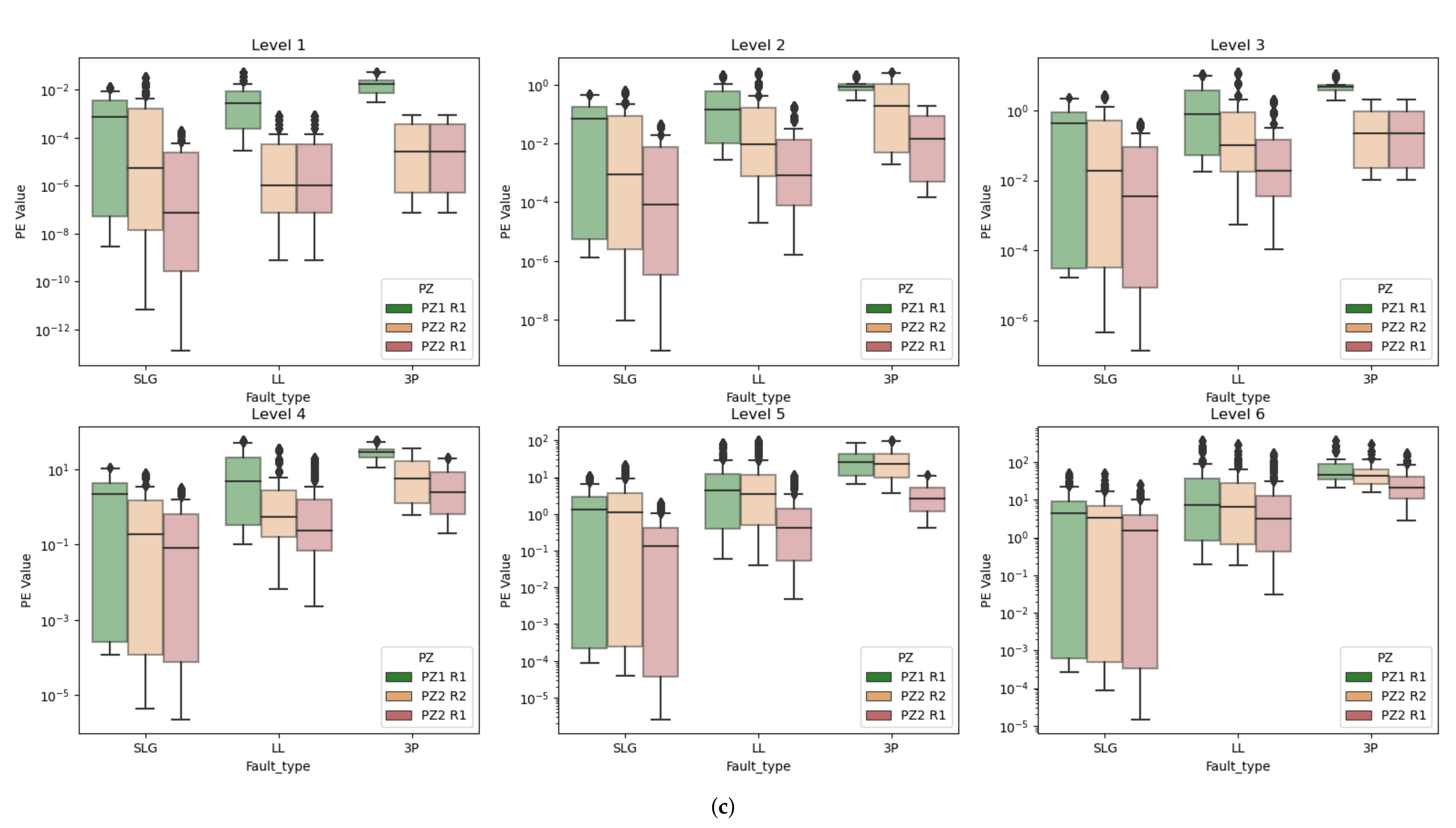
However, looking at the aerial modes in Figure 7b,c, the observations are the opposite: for faults in the next protection zone (PZ1 R1 or PZ2 R2), LL and 3P faults have more energy than SLG faults. For both aerial modes, and for all decomposition levels, LL and 3P faults’ energy magnitudes are consistently one or two orders of magnitude greater if looking at the distributions’ median. This observation can be related to the fault topology itself and the subsequent mode decomposition: the perturbation produced by an SLG fault (which directly affects one of the phases and indirectly affects the other phases due to the mutual coupling) is magnified when calculating the ground mode. However, the perturbation created by LL and 3P faults is partially canceled in the ground mode (or, at least, this can be observed for the TW within the first 50 $\mathsf{\mu }$s after the fault detection). On the other hand, the perturbation created by LL and 3P is adequately represented on the aerial modes. It is interesting to see that LL faults are more energetic that 3P faults in the Aerial 1 mode, but the opposite happens in the Aerial 2 mode.

The rate of attenuation due to distance is not the same for ground and aerial modes. This idea has been previously exposed in [19]. The coefficient of attenuation is larger for the ground mode than for the aerial modes. Regardless, the attenuation coefficient remains much more constant in the aerial modes than in the ground mode, in which, higher frequencies suffer from an exponentially higher attenuation. Taking the example of SLG faults, in the ground mode and for the first level, the average energy is four to eight orders of magnitude smaller when the fault is not on the next protection zone. For Level 6 of decomposition, which corresponds to much lower frequencies, this difference is just one or two orders of magnitude. Therefore, attenuation in the ground mode is severe, especially on the highest frequency bands. However, for the first aerial mode, for example, the difference in attenuation is between two and three orders of magnitude for SLG faults outside the protection zone for Level 1, whereas, for Level 6, it is not even an order of magnitude. This leads to a really important conclusion: if the distance is one of the most relevant factors in TW propagation in distribution systems, the ground mode is probably the most insightful mode, as it shows the effect of attenuation due to distance in a more significant manner.

For LL and 3P faults, attenuation seems similar both in the ground mode and in the aerial modes. However, this leads to an interesting paradox: LL and 3P faults are under-represented in the ground mode, where attenuation is relatively more evident (but still much smaller than for SLG faults). However, most of their energy is contained in the aerial modes, where attenuation is less patent. This fact will make LL and 3P faults more difficult to handle.

6. Conclusions

In this work, the authors have conducted an analysis of the most important factors for Traveling Wave (TW)-based power system protection related to the fault energy signatures in the first 50 $\mathsf{\mu }$s after the fault detection.This paper is motivated by the fact that, in most of the distribution power system protection works in the field, there is a low understanding of TW propagation in distribution systems. Most other works just use TWs for fault detection or location, without paying attention to how the existence of certain system elements affects the TW propagation, or how these energy values change as the system varies. This work studies the TW propagation on a test distribution system according to the following factors: distance, fault type, and the participation of certain elements in the system (extra laterals, extra branches on the protection zones, capacitor banks, and regulators). Several participation schemes of these elements are used in the model, and the associated energy values for these combinations are analyzed in the paper. The most important factors are outlined by a qualitative study of the TW energy variations.

In order to obtain those energy values, the faults have been detected using Dynamic Mode Decomposition (DMD), and, then, they have been decomposed into independent modes using the Karrenbauer Transform (KT). Due to the close relationship between the TW propagation and their frequency content, the Stationary Wavelet Transform (SWT) has been applied to achieve a time–frequency decomposition of the signals. The Parseval’s Energy (PE) theorem has been used to calculate the signal’s energy.

The results showed that a significant attenuation still occurs in distribution lines, significantly lowering the wave energy from distant faults. Regarding system elements, the presence of a regulator causes the most relevant drop in the PE values. This occurs either if the TW directly crosses the regulator or if there is a regulator somewhere upstream of the considered protection zone. Regarding the effect of laterals, the associated TW energy drop is maximized when the laterals are close to the fault location. Adding extra branches in protection zones leads to the same conclusions, lowering the PE values, especially if the fault location is close.

The analysis of the PE values per fault type provides several important insights: the ground mode seems to be the most prone to attenuation, which should lead to a more accurate fault location. This approach is especially suitable for Single-Line-to-Ground (SLG) faults. However, the relatively lower magnitude and attenuation on the ground mode for Line-to-Line (LL) and three-phase (3P) faults seems to suggest that those faults are not fully represented by the ground mode. On the contrary, the magnitude of the energy for LL and 3P faults is larger on the aerial modes, which are less subject to attenuation. These different patterns for SLG and LL/3P faults suggest that these faults should be handled by different approaches, and that LL/3P may be more difficult to work with, as attenuation due to distance (which seems to be the most important factor overall) is less evident in those particular fault types.