1. Introduction
An electrification of road transport has the potential of achieving near-zero emissions of greenhouse gases in the long term, i.e., assuming the electricity supply system is transformed towards carbon neutrality [
1]. While there is an ongoing electrification of passenger cars, mostly through battery electric vehicles, electrification of heavy transport, such as trucks and buses, still faces challenges due to the batteries required being heavy and occupying space [
2]. To drive for 4 h without a stop, a heavy truck would require a battery with capacity in the range of 600–800 kWh. With current battery technologies, such a battery package would weigh several tons. It is of course not known to what extent development in battery technology can reduce the weight of batteries, but it seems unlikely that there will be a large drop in weight over the foreseeable future. An alternative to large batteries is to supply the vehicles with electricity while driving, the so-called electric road systems (ERS). ERS may be able to supply enough power for heavy transport as they traverse the roads and thus reduce the need for large batteries. To reduce the size of the battery, it would require large-scale implementation of ERS on a national, and even European, scale. This will be associated with high up-front investment costs which will be paid by the user during the lifetime of the ERS. Additional equipment is needed on the vehicle to be able to use the ERS, but the investment cost and the maintenance cost of this equipment is small compared to the battery cost [
3]. ERS has gained a political interest during recent years in Sweden and Germany. An important factor for ERS deployment is their economic and technical feasibility, requiring investments in new infrastructure but lower vehicle costs due to reduced battery sizes [
3]. Furthermore, Taljegard et al. [
4] shows that the potential to reduce CO
2 emissions from road traffic using ERS is significant, even if implementing ERS on a minor share of the Swedish road network.
The ERS concept can be divided into three main technology groups: (i) the vehicle fleet, (ii) the electric road infrastructure, and (iii) the electricity supply to the electric road infrastructure. The electricity supply system to the road infrastructure consists mainly of substations that transforms from high voltage to medium voltage, cables that supply electricity from the regional grid to the electric road infrastructure, and power boxes with rectifiers that converts electricity from AC to DC. Power boxes are typically placed every 40 m along the road [
5]. Electricity can be supplied to the vehicle by overhead transmissions or from the ground (road). The electric road infrastructure can be either overhead transmission technologies that are conductive-based with the vehicle connecting to the transmission lines by a type of pantograph (successfully demonstrated outside the city of Gävle in Sweden) or ground-based technologies that can be either conductive or inductive [
6]. When conductive, the supply is through a physical pick-up to connect to an electrified rail in the road (currently demonstrated in the city of Lund and has been demonstrated outside the city of Stockholm, Sweden) [
7]. Inductive supply is achieved by using a wireless power transfer from a coil in the road to a pick-up in the vehicle (and is currently being demonstrating outside the city of Visby on the island of Gotland, Sweden) [
7]. Regardless of the electric road infrastructure technology utilized, a connection to the existing high-voltage grid is needed.
ERS is a relatively new concept, and therefore, there is limited amount of research performed on the topic. Historically in the scientific literature, a large focus has been on technology improvements of the ERS road infrastructure, such as the inductive charging system efficiency [
8], alignment tolerance of the inductive power transfer transformer [
9], and the efficiency of an AC-conductive ERS [
10]. There have also been studies on life-cycle assessments of ERS, such as Marmiroli et al. [
11], Balieu et al. [
12], and Schulte et al. [
13]. Furthermore, several studies modeling the impact of ERS on investment in the electricity power system have been conducted, such as Taljegard et al. [
14], Olovsson et al. [
15], Coban et al. [
16], and Plötz et al. [
17]. The power system implications and power systems related costs of ERS have not been thoroughly investigated. Power grid assessment of new technologies, such as static EV charging [
18], renewable energy sources [
19], and solar photovoltaic technologies [
20] have been given considerably more focus.
Furthermore, several studies have investigated the cost of building an ERS and compared it to other alternatives to decarbonize the transport sector. Márquez-Fernández et al. [
3] found, when studying a large-scale deployment of ERS in Sweden, that a scenario with widely used ERS at the highways will have a lower system cost than static charging infrastructure. In their study, it is assumed that the battery size of the truck can be reduced from 500 kWh to 75 kWh with widely used ERS. Coban et al. [
21] came to similar conclusion when analyzing two scenarios, with and without ERS, for Turkey. Börjesson et al. [
22] performed a cost
–benefit analysis of ERS in Sweden. They found that for an ERS in Sweden the social benefits are larger than the social costs and that the ERS can significantly reduce carbon emissions from heavy trucks. Taljegard et al. [
4] came to a similar conclusion from an analysis of the potential for ERS to reduce CO
2 emissions in Norway and Sweden. Connolly [
23] also found ERS to be cheaper than BEV for electrifying heavy road transport. However, none of these studies applying cost analysis focused on the cost or components in the electric supply system to the grid.
The cost of investment in infrastructure needed for an ERS remains uncertain, with costs ranging from EUR
2016 0.4 to 5 M per km reported in the previous literature (Domingues-Olavarría et al. [
24], Sundelin et al. [
25], Olsson et al. [
6], Asplund [
26], Wilson [
27], and Boer et al. [
28]). These studies give either a total cost for building ERS (per km) or a cost separated between cost for vehicle components, the electric road infrastructure and the electricity supply system to the electric road infrastructure. However, none of the studies reports detailed component costs for the electricity supply system to the electric road infrastructure.
In a case study by Hjortsberg [
5], the cost of building an ERS using the road E4 in Sweden was analyzed in more depth compared to the previous mentioned studies, with the help of two power utilities (Vattenfall and E.ON). Hjortsberg [
5] found the cost for the electricity supply system to the road infrastructure to be approximately SEK 8 million Swedish Krona (SEK) per km (corresponding to EUR
2022 0.74 M using an exchange rate of EUR 10.75/SEK). The latter compared the investment cost for two cases; an extension of the regional 130 kV grid and the construction of a new 30 kV grid next to the road. While the study by Hjortsberg [
5] is technically and geographically relatively detailed in its connection to the already existing regional grid, it also has a few limitations: (1) it applied a fixed distance of 40 km between the substations while varying the power delivery by each substation according to road demand, (2) it does not consider voltage drop in the substation placement procedure, and (3) it does not consider total cost of ownership that includes electricity losses in the ERS due to substation placement and component choice. This means that Hjortsberg [
5] is likely to underestimate the power supply needed for the road, and thus the size of the substations and maximum spacing allowed between substations. Li Yu et al. [
29] presents a theoretical framework to determine the optimal location of substations considering the cost of land. Silvia et al. [
30] proposes a new method based on artificial immunological systems for solving the problem of substation allocation in distribution systems. However, none of the studies are applying the framework to an ERS.
In summary, previous studies have produced widely different cost assessments of ERS, and they have largely used a case-based approach where it is unclear how generalizable the cost assessments are as well as how they are impacted by specific parameters of the relevant case. Important parameters are the demand pattern of the road, including the variation of demand along the road as well as assumptions of how the ERS infrastructure is built with a focus of sizing and placement of substations and cables.
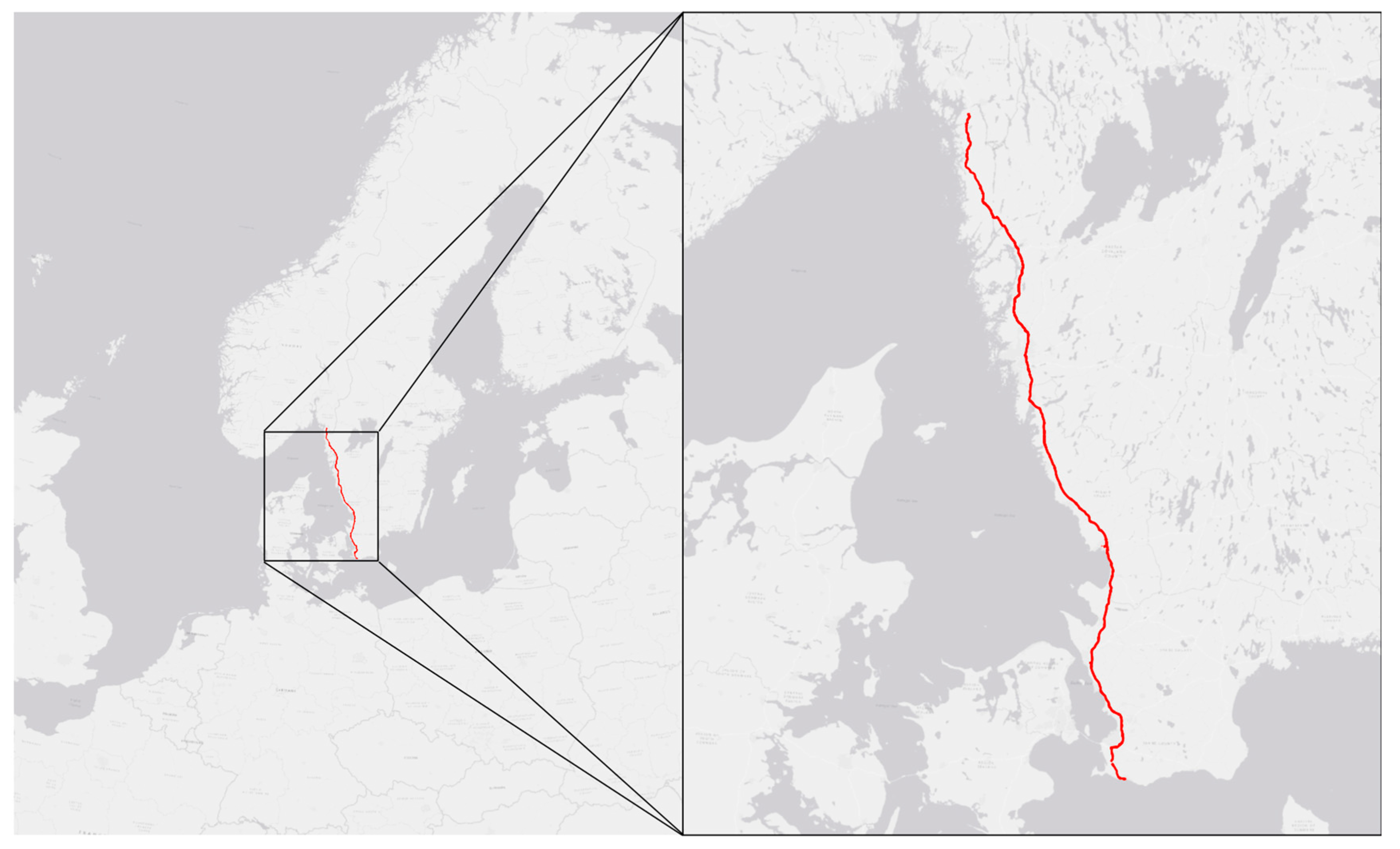
The aim of this study is therefore to systematically investigate the impact from (1) substation placements and size on the ERS electricity supply system costs while considering technical limitations in the grid such as electricity losses, voltage drop and thermal capacity of components and (2) the impact of variations in the power demand of the road and its effect on total cost for the ERS. A model has been developed that calculates cost for supplying an ERS with electricity from a regional grid to a road in the form of cables and substations, considering the power demand profile for heavy transport. The modeling accounts for electric losses and voltage drop in cables and transformers. This study is based on data for the European Highway 6 (E6) in western Sweden (see
Figure 1 for a geographical map). Where we have varied the average demand and the peak power demand to investigate how sensitive the results are to a specific road, and a specific demand pattern. Therefore, our results are of general interest for electric road analyses. As seen in
Figure 1, E6 connects several big cities in Sweden. ERS will benefit both the cities and country-side.
2. Methodology
In this paper, a model to calculate the cost for building a medium voltage (30 kV) grid supporting an ERS is developed. The model consists of two modules: (1) a model based on the technical requirements of the grid that supplies power from the regional high voltage (130 kV) grid to the road, i.e., power demand, power losses, voltage drop, and n − 1 criteria (
Section 2.1) and (2) an economic model that calculates the total cost of ownership (TCO) for the ERS distribution system (
Section 2.2).
Figure 2 shows a schematic overview of what is included in the technical and economic models. As seen in
Figure 2, this study disregards costs for the parts of the ERS that will be constant with varying placement of substations, i.e., (i) costs for ERS road infrastructure, i.e., the rail in the road or overhead lines that is used for power delivery to the vehicles, and (ii) costs for power boxes. Furthermore, since the current locations of 130 kV substations are publicly unavailable, we exclude the 130 kV grid extension in the model. An important assumption that underlies this work is therefore that there exists a regional grid close to the road that is to be electrified and that this grid has the potential to supply enough power for the ERS demand. According to Professor Per Norberg in Vattenfall, the assumption of a regional grid close to the road is fulfilled for E6 [
31].
A major issue when considering what impacts the location and size (and thereby number) of substations and associated cables has on ERS cost is to account for the many possible combinations of locations and sizes. With the six different sizes of substations used by Hjortsberg [
5] (16, 20, 25, 30, 40, and 50 MVA), this results in between roughly 10
8 and 10
26 different combinations of substation sizes and locations that are able to fulfil the road demand under the aforementioned technical requirements. Ideally, we would compute all possible combinations of substations and sizes and thereby gain an understanding of how much, and in what way, the cost for the ERS can vary with substation locations. This is unfortunately computationally unfeasible. Instead, we do two other things.
Firstly, we calculate the annualized cost for a large set of different substation placements and sizes along the road and argue that this subset is representative of the whole solution space. By representative we mean that it is unlikely that solutions exist which have a much lower or much higher cost compared to what we have already found and that the distribution of possible costs that have been computed is unlikely to change compared to if we had computed all possible solutions. Specifically, we pre-generate a large number of random sequences of substations that the model places along the road, using the same possible sizes as in Hjortsberg [
5]. The technical criteria, i.e., power demand, power losses, voltage drop, and n − 1 criteria, limit how large a part of the road one of the substations can supply power for. The model systematically places the substations along the road E6 from south to north, as far apart as possible, while still fulfilling all of the previously mentioned technical criteria. The model checks if the technical criteria are fulfilled for every km of the road while traversing the road from south to north. As soon as one of the criteria is unfulfilled, the model places a new substation from the pre-generated list at this location.
Secondly, we observe that it is indeed possible to compute the annualized cost for all possible combinations of substations and sizes for a shorter road than the E6. In this case, we choose to only electrify the southern half of E6 and exhaustively compute all possible combinations of substation placements that supply the demand under the aforementioned technical criteria for this part of the road, and an additional constraint is that we exclude the smallest size of substations (16 MVA) in order to make the computation feasible. Including the 16 MVA option would increase the size of the solution space and significantly increase computational time, while it is the least favorable transformer size due to a high cost per MVA ratio. We obtain all possible combinations of substations and sizes by computing the n-fold Cartesian product of the set of possible substation sizes and where n is the number of substations required to electrify the road if only the smallest substation is allowed. Again, the substations are placed as far apart as possible from south to north, while still fulfilling the previously mentioned technical criteria. When the road is fully electrified, we stop placing substations from the pre-generated lists, even if all n stations have not been used (since the Cartesian product will always give lists of length n, even though n substations will not be required if some substations are large).
We will show that the conclusions from the two methods are similar, thus providing robustness of the research findings.
Section 2.1 describes the technical constraints for the grid that supply power to the road and the impact of substation placement along the road, while the economic costs of electricity losses are described in
Section 2.2.
2.1. Electric Grid Model
There are several factors to consider that can limit the positioning of substations along the road and thereby impact the cost of the distribution system between the regional grid and power boxes: (1) voltage drop along the 30 kV cables; (2) time constraints of earth switching (“tripping criteria”); (3) reliability criteria; and (4) thermal capacity of components such as cables and transformers. Generally, losses increase with the square of the current, thereby pushing for fewer substations. Simultaneously, voltage drop increases over distance, which favors many substations.
The model assumes simplified power system calculations for voltage drop and losses. We exclude the earth switching criteria and harmonics in the model as it is likely that these have small impacts while requiring significant additional model complexity [
32]. Distribution related reliability criteria can be implemented by using different grid topologies or by adding additional equipment. We consider n − 1 as a criterion for reliability in the distribution system. The n − 1 criterion is fulfilled by setting the requirement that each station (and cable thickness) should be able to supply power all the way to the previous and next station.
In line with previous work, the model accounts for active losses. Even though there are reactive losses, it is assumed that they can be compensated for in the inverters. Active power losses are calculated as:
where
I is the current for each section of km,
R is the resistance for the cable (
r is the resistance per km of the cable and
l is the length of the cable). Data on resistance are taken from ABB sales data [
33]. Cables refer to isolated electricity conductors that are placed underground.
A simplified model for voltage drop is used. Voltage drop is regulated to not be above 10% in a given system but is often designed with stricter criteria. We assume a design criterion for maximum voltage drop to be 5% from one substation until the location where it is used; the reason for this strict voltage drop requirement instead of, e.g., 10% is that we thereby also account for possible voltage variation in the supplying grid. Voltage drop can be calculated as
where
X is the reactance,
P is active power,
Q is reactive power, and
is nominal voltage. We use a short line model (line length < 80 km and
69 kV), which excludes any capacitive part of the reactance. The reactance can then be calculated as
where
f is the frequency in the grid (50 Hz in Sweden),
L is the cable inductance (obtained from ABB sales data [
33], and
is the line length. The active (
P) and reactive (
Q) power are calculated as
where
is the cable voltage for km
,
I is the load current for km
, and
is the power factor (assumed to be 0.9). The power factor describes how apparent power is divided into active (kW) and reactive (kVAr) power.
The substation capacity is set as an input variable from pre-generated sequences of stations. In the model, the road is traversed from south to north, and at every discrete km step each of the preceding technical criteria is evaluated, and if one of them is no longer fulfilled using the preceding substation, a new substation from the pre-generated lists of stations is placed 1 km to the south of the point of evaluation (to ensure that the n − 1 criteria is fulfilled). From each substation, cables are assumed to extend in each direction of the road. The cables must be rated for a line current (
) equal to half the transformer capacity, which becomes
where
is the transformer capacity rating in volt-amperes.
2.2. Economic Model
We consider the total cost of ownership (TCO) when comparing costs for different substations placements and sizes. The TCO consists of two parts, the investment cost for substations and cables, which is annualized with the capital recovery factor (CRF), and the cost for energy losses in the system (see Equation (7)).
The capital recovery factor is calculated as
where
r is the discount rate, set to 5%, and
T is the investment horizon. Different components in the grid have different lifetimes, generally 40 or 50 years. We assume an average of 45 years for the system yielding a CRF of 0.0563. The costs for different components are taken from a list of standard costs from the Swedish Energy Market Inspectorate [
34].
The annual cost for energy losses in the system is based on the electricity losses, obtained from Equation (1), using average demand over a year multiplied by the number of hours in a year. Electricity losses from transformers are excluded due to lack of data of transformer impedance. However, the total transformed power is about the same in all configurations (some tens of % above road demand). Since transformers are sized based on the road demand, they have similar levels of loading in all configurations. Impedance losses in the substations should therefore be similar in all configurations and can be disregarded for our purposes of comparing placements of substations.
The substations costs include costs for groundwork, switchgear, 2 × circuit breaker (input side and output side), and transformers (see Equation (9)).
For the sizes of substations used here, only transformer costs change with size, unless more than six transformers are used, then a larger switchgear (a single switchgear have space for up to six transformers) is needed. This means that the cost of a substation is reduced with increased capacity, which depends on the converted MVA. An exception is when the largest 50 MVA (2 × 25 MVA) substation is used, as this setup requires two slots in the substation. In reality, a substation also includes additional equipment such as remote-control apparatuses and additional safety features. The costs for these are likely much smaller than other cost mentioned and are therefore disregarded. The cost parameters are available in
Appendix B.
Hereinafter, we use the term “modeled cost” to refer to the annualized included costs for the ERS, and these costs are thus the sum of all substations (groundwork, switchgear, circuit breakers), all cables, and all energy losses for the entire ERS. Costs for power boxes, overhanging lines, etc., are still excluded when using the term “modeled cost”. We will also refer to “cable cost”, “energy loss cost”, and “substation cost”; in these cases, the cost is also annualized, and the sum of these three costs equals the “modeled cost”.
4. Results
In
Section 4.1, we present the results for the solution space validation where 10 million trials are compared with 100 million trials. In
Section 4.2, analysis of the main scenario is presented. The section includes results on the spread in different costs (substation costs, cable costs, and energy loss costs) for three scenarios for the whole road (Case 1) and the same three scenarios for half the road (Case 2), where all solutions are computed for Case 2, and 100 million solutions are computed for Case 1.
Section 4.3 contains an assessment of the effect of including the voltage drop criteria in the analysis.
4.1. Solution Space Validation
Here, we compare the obtained sum of annualized substation, cable, and energy loss costs in a trial of 10 million random configurations to that of 100 million random configurations with the purpose of determining if we explore a large enough portion of the solution space to draw general conclusions of how costs vary with substation placement along the road. We do this by comparing the lowest and highest modeled cost for the tested configurations and by comparing the distribution of modeled cost for the two trials, shown in
Table 1. As shown in
Table 1, the differences between 10 million and 100 million trials are small, with the lowest cost falling at 0.56% in the 100 million trial case compared to the 10 million trial case, and the highest cost increasing 0.38% in the same comparison. This suggests that 10 million trials yield a sufficiently large proportion of the solution space; however, in the following sections we will use the 100 million trial case when considering the whole road.
4.2. Distribution of Costs with Respect to Power Demand Profile
To determine the impact of the road demand profile on the distribution of costs, we vary the demand profile according to three schemes to capture possible different impacts in the costs produced by the model. The three schemes are:
- S1.
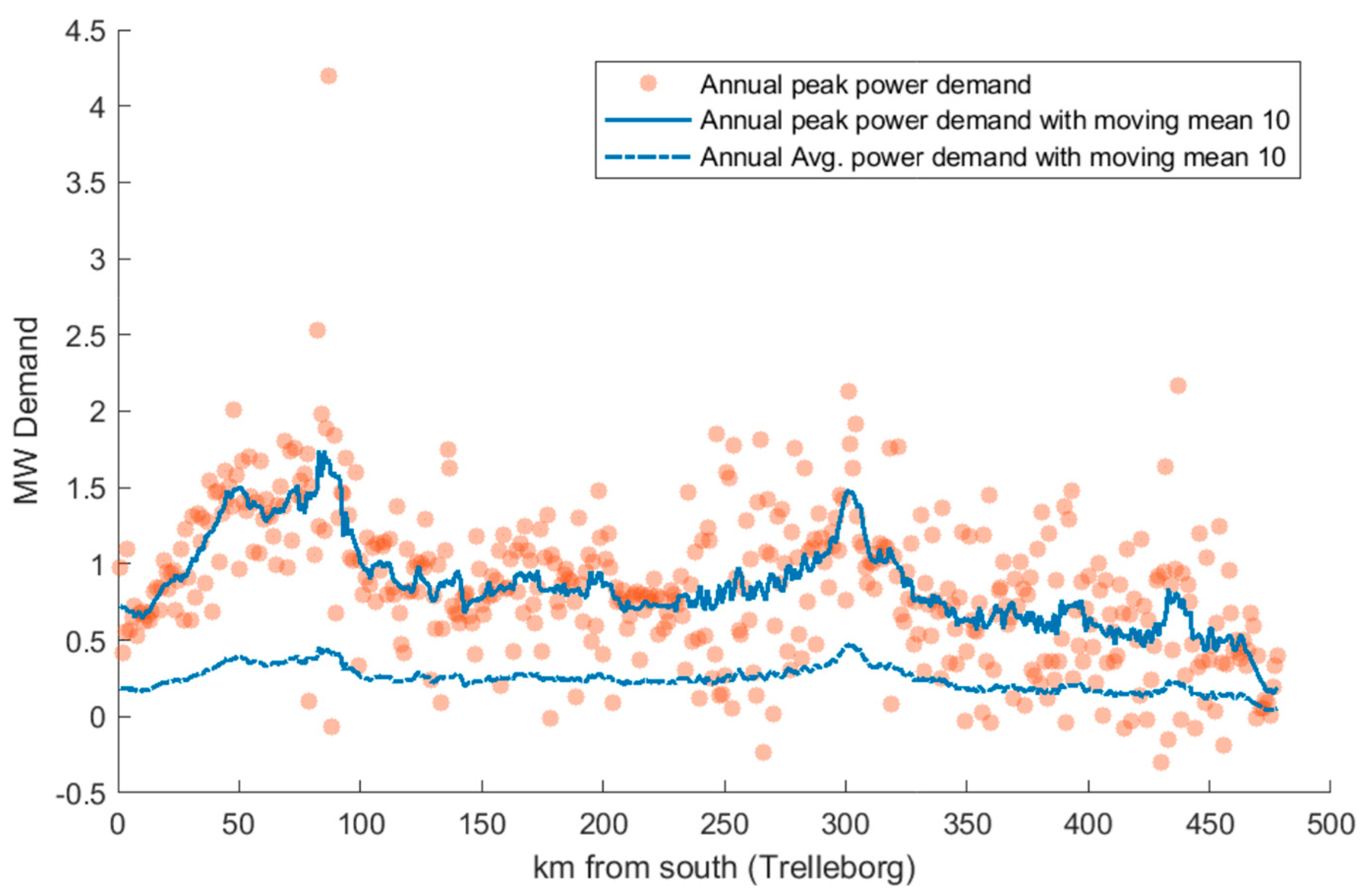
The peak and average demand is multiplied by a fixed factor (smaller than 1) over the whole road, i.e., all curves in
Figure 3 are shifted down. Thereby, both the average demand and the peak demand for the road are decreased.
- S2.
The difference in peak and average demand along the road is reduced, i.e., the peaks and valleys in
Figure 3 are shifted closer to the mean. The mean is kept unchanged, so that the summed power demand along the road is unchanged.
- S3.
Peak demand is multiplied by a fixed factor (smaller than 1), while the average demand is kept unchanged, i.e., the peak demand curve in
Figure 3 is shifted down.
The effect of the three schemes on the demand are visualized in
Figure 4.
Figure 5 shows the cost per substation (bottom right panel), cable (top right panel), and electricity losses (bottom left panel) as well as the sum of these three costs (top left panel), i.e., the modeled cost. The configurations in all panels are sorted from lowest to highest modeled cost, and each panel shows results for the original demand profile as well as the three adjusted demand profiles using an adjustment factor of 0.7. The individual cost panels (cable, loss, and substation costs) have been smoothed with a moving mean of 5000 configurations. Therefore, these should only be used for determining relational trends between the individual cost components as modeled costs increase, relational trends between the original demand profile, and the three demand variation scenarios. They should not be interpreted as showing a specific cable/substation/loss costs for a specific modeled cost. The specific non-smoothed costs for these three panels vary significantly in-between neighboring configurations (“neighboring” meaning configurations with the closest modeled cost) making a graphical interpretation of the relationship between the scenarios difficult. The summed costs follow an S-pattern, with a few low-cost configurations, a few expensive configurations, and the large majority having a similar modeled cost. We observe in
Figure 5 that the cable costs represent the largest cost, followed by substations and finally electricity losses; electricity losses are also small and relatively constant regardless of substation configuration. The large variation in costs between configurations for each of the cost components (electricity losses, cable, and substation) suggests that there is a large freedom in choosing a configuration that has a low cost for one of the cost components while also having a high cost for one of the other cost components.
When considering the original demand profile (i.e., S0), we observe that a large number of substation configurations yield a similar modeled cost. This suggests that it is hard to find heuristics for substation placements that have the lowest cost. The substation locations with the lowest modeled cost have a cost which is 10% lower compared to the average cost of all configurations. However, note that these costs are only those that vary with substation placement. The full cost for an ERS also includes power boxes, rectifiers, over-hanging lines at the road, and possibly an extension of the 130 kV regional grid to the road, thus making the impact of an optimal substation placement relatively small compared to the full cost of an ERS. The upfront investment cost (substation cost plus cable cost) for the 478 km is on average SEK 1.90 M/km and the lowest upfront cost is SEK 1.70 M/km. This variation in installation costs due to substation placement can be compared to the full cost for the ERS of SEK 8 million per km that was estimated by Hjortsberg [
5].
When considering the demand variations (S1–S3), we observe that S1 and S3 lower the total costs across the solution space. This is mainly a result of the reduced peak demand, as peak demand sets the constraint for how many and how large substations that are needed to satisfy the demand. The S2 scheme has a somewhat lower substation cost than the original demand, which also causes it to have a slightly lower modeled cost compared to S0. However, it is noteworthy that the impact on modeled cost is low in the S2 case, where the demand profile has been changed, but peak and average demand remand unchanged. This suggests that peak power demand largely is the only relevant factor for determining the cost of an ERS (assuming a nearby regional electricity grid) and not the profile of the demand curve. Cable costs only vary to a small extent in-between the different scenarios. While cost of losses vary more, their contribution to the modeled cost remains low irrespective of scenario.
Figure 6 displays the cost results from all possible combinations of substation placements when using only half the road. The layout of the panels and scenarios are the same as in
Figure 5. We observe that the modeled cost for the original demand profile and the three varied demand profiles relate to each other as in
Figure 5, where specifically S1 and S3 have a lower modeled cost compared to S2 and the unchanged demand curve. The panels of the three separate cost categories are significantly noisier compared to the previous case; however, the combined modeled cost varies approximately as much from the low cost cases to the high cost cases as in
Figure 5. Additionally, the possible substations costs in
Figure 6 vary slightly more compared to
Figure 5. This suggests that the option to choose substation sizes and location, while still having the same modeled cost is even stronger than in the case with the whole road. This could be an outcome from not having computed all possible solutions in the case where we use the whole road. Otherwise, the three separate cost categories are impacted by demand profile variations in the same way as in the case when including the entire road.
The main conclusion from varying the demand profile according to the three schemes (S1–S3) is that a change in the peak power demand for every substation along the road has the largest impact on cost. Combined with the previous results of this paper, that costs vary only a little with substation placement (in relation to the full cost for the ERS), this suggests that the cost for constructing an ERS can be reasonably expressed as a function of only peak power demand. This may be valuable in applications where ERS costs are compared to its benefits in various situations, such as in energy system modeling. Yet, this is dependent on the assumption that there is a nearby regional grid with sufficient capacity.
Additionally, substation placement appears to only have a small impact on costs. This could be beneficial when considering the extension of the regional 130 kV grid. If technical limitations, such as the location of the regional grid in relation to the road, hinder the cheapest alternative, then the planning of substation placement would yield only small cost savings.
4.3. Impact of Voltage Drop
Table 2 shows the modeled cost for two transformer configurations, 50 MVA (large) and 20 MVA (small). This is to show the difference in result of having fewer, and larger, substations compared to having many small substations. Furthermore,
Table 2 shows the effect of including a voltage drop criteria for placing substations and including losses; note that a restriction of only using a fixed MVA per station leads to some over-capacity, but the purpose here is to illustrate the effect of voltage fall.
In
Table 2, it can be observed that 25 substations of 20 MVA each is required to meet the peak demand of the road, while for 50 MVA sizes it is sufficient with 9 substations. We further observe that for the large substations the effect of including voltage drop on the full costs is positive (increased modeled cost), while for the small substations the effect is negative (reduced modeled cost). In both cases, the change in modeled cost is small. This is likely due to the increase in distance between larger substations. As seen in
Table 2, including voltage-drop criterion increases the required number of substations from 9 to 11 for 50 MVA capacities; the inclusion of voltage-drop also increases the modeled cost from SEK 53.92 million to SEK 57.60 million. However, it should be noted that in the most expensive case, there is one station placed just a few km from the end of the road, thus suggesting an over-investment in substation capacity in this case. The results that voltage drop play a larger role for larger substations and longer cables is also consistent with the theory presented in
Section 2.2.
Figure 7 shows the peak demand profile overlaid by the positions of substations in a configuration with only 50 MVA substations.
5. Discussion
The purpose of this study is to two-fold, where we have (1) investigated the impact from substation placement and size on the ERS electricity supply system cost while considering technical limitations and (2) have investigated the impact of demand pattern variation on the cost for the ERS. Our methodological approach has been to investigate a large number of substation placements that fulfill the technical limitations and evaluate their cost. As a comparison, it would also be interesting to find the lowest cost via optimization. However, such an approach is challenging due to two technical aspects. The first aspect is that the optimization will be non-linear when including electricity losses as a limiting factor for substation placement. This is due to electricity losses depending on the square of the current, which in turn depends on road demand. The second aspect is that sizes of substations and cables are non-continuous, thus requiring mixed-integer optimization which can be computationally infeasible. A reasonable approach for optimization is to make the problem linear by removing electricity losses as a placement criterion and instead only place substations according to power demand and voltage drop. In general, we found that the voltage drop restricts the placement of substations.
In this study, Swedish data were used for cost parameters for substations and cables. In an international perspective, costs may vary, although it is likely that expensive components, such as transformers and switchgear, are of comparable cost across international markets. Labor-intensive costs, such as cabling and groundwork, are more likely to vary depending on region. The variation in labor costs would need to be large in order to impact the main conclusion of this study, i.e., that substation placement has a low impact on the cost for building an ERS. Even though we have included most costs in the distribution grid extension of the regional grid, certain components, such as monitoring and safety systems, have been excluded. The exclusion of such components likely has a minor impact on overall costs and, as such, should not affect the conclusion in this study. The minor impact is likely due to two aspects. First, the cost of additional equipment is small compared to the overall costs of substations and cables. Second, the additional costs are less influenced by substation placement than transformation capacity and cables.
Overall, there are three main uncertainties that are relevant for this work. These are (1) uncertainties regarding the power demand profile, (2) uncertainty regarding substation placement, (3) uncertainty regarding component costs and electricity cost. The first two of these uncertainties are an integral part of the analysis and were therefore considered. The cost uncertainty is not modeled explicitly; however, it is possible to reason around the effect of cost uncertainty. All the included components can be divided into three categories (substation related cost, cable cost, and electricity cost); in addition to these three categories, the assumptions on component lifetime and the discount rate can be varied. The three base-cost components (substation, cable, and electricity losses) scale linearly with changes to the underlying cost assumptions, and therefore they do not alter the general conclusion that costs only vary minorly with substation placement and demand pattern variation. Discount rate and component lifetime scale non-linearly; however, they only impact the relative importance of electricity loss cost vs. substation and cable costs. Therefore, they also do not impact the general conclusions of the paper.
We found that many different configurations of substations yield a similar modeled cost. This may depend on the assumption that a regional grid (130 kV) is available close to the road (which is the case for our example of the road E6). An extension to the 130 kV grid was not included in the cost calculations in this study. If this assumption is not the case, e.g., not having the regional grid available for a stretch of road, or for the whole road, then it is possible that the model would favor larger substations that supply power to longer stretches of the road. Additionally, the assumption to set the roadside grid at 30 kV may also impact electricity losses, substation costs, and cable costs. The decision to use 30 kV is due to that this complies with commonly used voltage levels in the Swedish distribution grid [
5] and allows sizing of cables to be within thermal capacity limits and voltage variation constrains. In reality, a road with a low peak power demand may benefit from a lower voltage level, while a road with higher peak power demand may benefit from an increased voltage level, thus introducing additional non-linearities into the model. These are all avenues for future research to explore. Further research could also consider losses from transformer substations, as well as the cost for connecting to the 130 kV grid. However, that requires knowledge of the placement and available capacity on the current substations. It would also be interesting to compare the difference in cost and benefits between cables and power lines.
The work has assumed that the sizing of an ERS would need to fulfill the n − 1 contingency criteria. In our case, this was implemented by sizing each substation and length of cable to supply the road demand for the full distance to the next substation. If an ERS is built for vehicles where the battery size is non-existent, the n − 1 contingency can be motivated. However, if the ERS purpose is to reduce the reliance on batteries, the criteria could be excluded. Regardless of if n − 1 is included or not, it is unlikely to impact the main findings of our study, that placement of substation has a small impact on overall costs. Excluding the n − 1 contingency would only reduce overall costs for all placements.
A specific result that would warrant additional investigation in future research is that the modeled cost does not change with reduced variation in peak power demand along the road (when aggregated peak power demand is maintained). It would be reasonable to assume that at some point the modeled cost would be affected, especially if the variation along the road is increased instead of decreased. With high enough increase, some stretches of road would reach near-zero demand, while other stretches would reach a high demand, and this could result in the need for very specific substation and cable sizes, that might impact the modeled cost. A main conclusion of this paper is that, given the assumption of a nearby regional grid, the cost for an ERS may be expressed as only a function of aggregated peak power demand for the road and note that this is true for the whole ERS cost including non-modeled costs such as power boxes and rails or over-hanging lines, since these costs are also either constant (overhead lines) or only dependent on peak power demand (sizing of power boxes). A natural extension of this study is to empirically determine this relationship. This could be achieved, for example, by assuming a low degree of electrification of the heavy transport on E6, or another road, and then increasing the electrification degree in small steps while computing the minimum and average modeled cost.


