The dynamic model for the problem at hand is summarized below. The situation being modeled is interesting in that we have floating-body oscillations being excited by waves, with the oscillations in turn exciting the oscillations of the flexible beams with magnetostrictive actuators attached. Thus, between the waves and the electric circuit powered by the actuator current and voltage, there are three energy exchanges: (i) between waves and floating body, (ii) floating body and oscillating beams, and (iii) beam oscillations to converter electrical circuits. The boundary conditions for the overhanging beams are summarized below.
2.2.1. Boundary Conditions
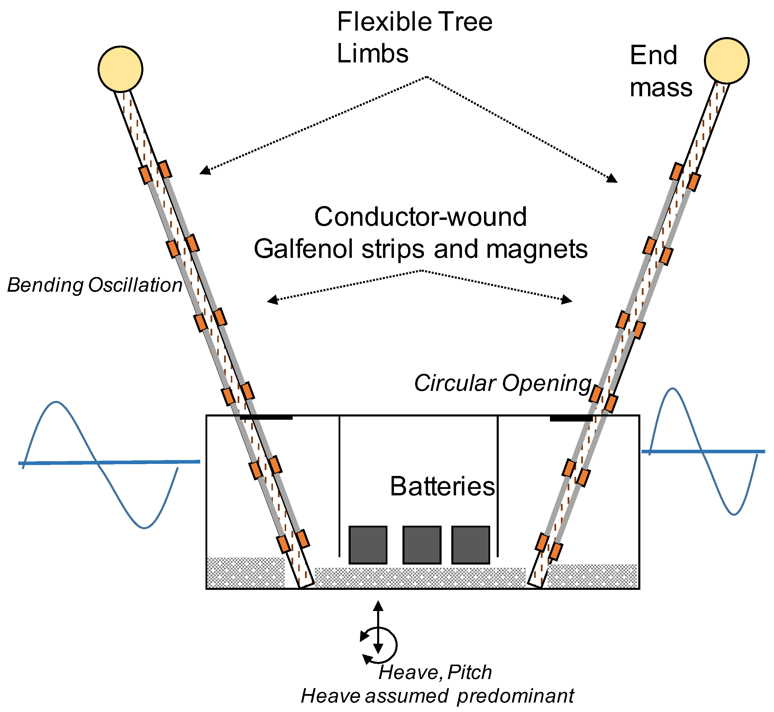
The tree limb beams shown in
Figure 1 are resting on the keel of the buoy, with part of their weight also being supported by the deck openings through which they overhang. Here, the two supports are modeled as pin joints, and the tree limbs are modeled as two-span beams with one span of length
overhanging a shorter simply supported span of length
. For either beam of length
, with
denoting the out-of-plane beam deformation at a point
x along beam length, we may define
, and
to express the beam profiles
for a solution
as follows.
Additionally, we allow below for the endpoints of the beam overhangs also to support an end masses to accentuate beam oscillations at the lower frequencies common to ordinary wave spectra. The boundary conditions become
above represents the end mass carried by each beam, and
represents the flexural rigidity of the beams with Galfenol strips attached.
is defined in the following section. The boundary conditions in Equation (
20) present a closed system, with the determinant going to zero at the spatial eigenvalues of the overhanging beams. From these, the natural frequencies of the beams can be determined for various geometries and end-masses, with the goal of finding the best combinations for the present application.
Two cases are studied below: (1) where the deck-level supports for the beams are tight enough for the beams to maintain contact with them throughout the oscillation; and (2) where these supports are loose enough for the beams to bounce within the supports during their oscillation cycles.
For convenience, the buoy shape is chosen to be cylindrical with a hemispherical bottom. Heave is assumed to be the dominant oscillation, even though a pitch/roll mode can be added relatively easily. For the case with the tight deck-level supports, the dynamic variables are (i) buoy oscillation in heave s, (ii) beam oscillations in single-axis bending , and (iii) voltage produced between the terminals of an electrical load circuit connected to the actuators V. A third variable representing the beam angle was added to the system for the situation with loose supports. It was found convenient to use the variational formulation for deriving the equations of motion for the entire system.
2.2.2. Beams Tightly Fitting through Deck Supports
For the first case, the angle between the beams and the vertical was assumed to be a constant,
. For the beams, uniaxial bending is assumed, and shear deformation and rotary inertia are neglected. The total kinetic energy was expressed as
The in-air mass of the buoy is
, while
represents its infinite-frequency added mass in heave.
is the mass of each beam, and
is the end-mass attached to each beam. Further,
is the deflection of the
ith beam perpendicular to its neutral axis, the vertical deflection component
being given by
. The strain at any beam fiber
z from the neutral axis can be expressed as
for small deflections. Then, using this expression for
S in Equation (
17), the total potential energy of the beams together with the potential energy of the buoy can be expressed as
Here,
denotes the second derivative with respect to
x of
, the out-of-plane deflection of the
ith beam. The Lagrangian
is
An action variable
J can be set up over a time interval
such that
Minimization of
J over the interval
requires that the first variation
. The minimization process leads to the equations of motion and the boundary conditions (natural or externally prescribed), which we here prescribe as in Equation (
20) above. The equations of motion can be derived from
The force
on the right side of the first of Equation (
25) represents the exciting/diffraction force due to waves, the radiation force due to body oscillation in waves, and additional effects such as viscous-frictional damping.
The equation of motion for the buoy is
on the right denotes the exciting force (accounting for diffraction effects) due to waves. The convolution integral on the left is part of the radiation force, with
denoting the impulse response of the body.
represents the linear approximation to the viscous friction damping force. Next, the equation of motion for the
ith beam is found to be
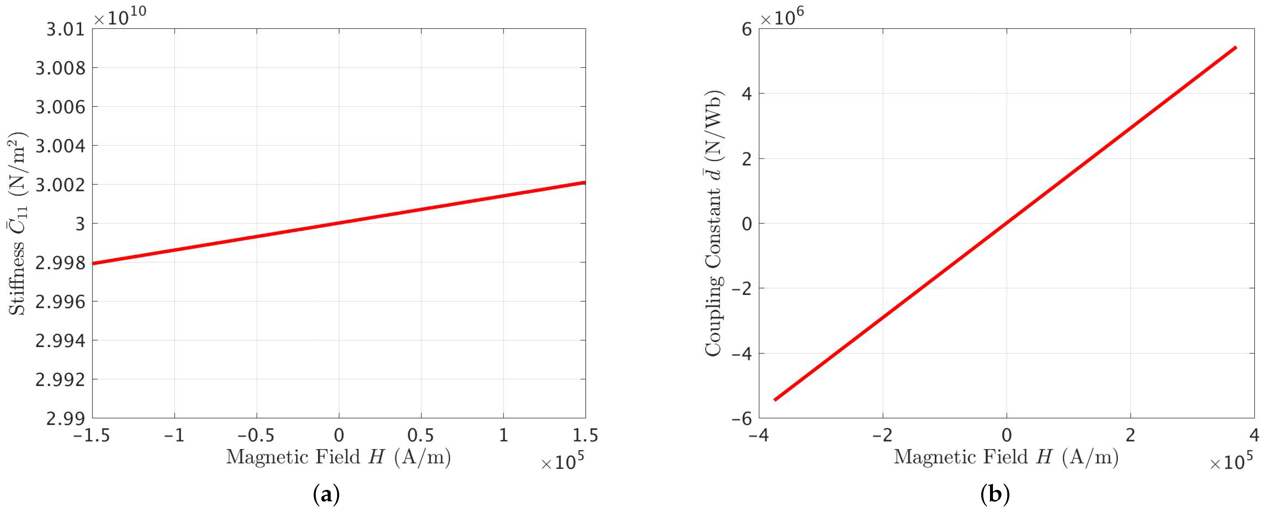
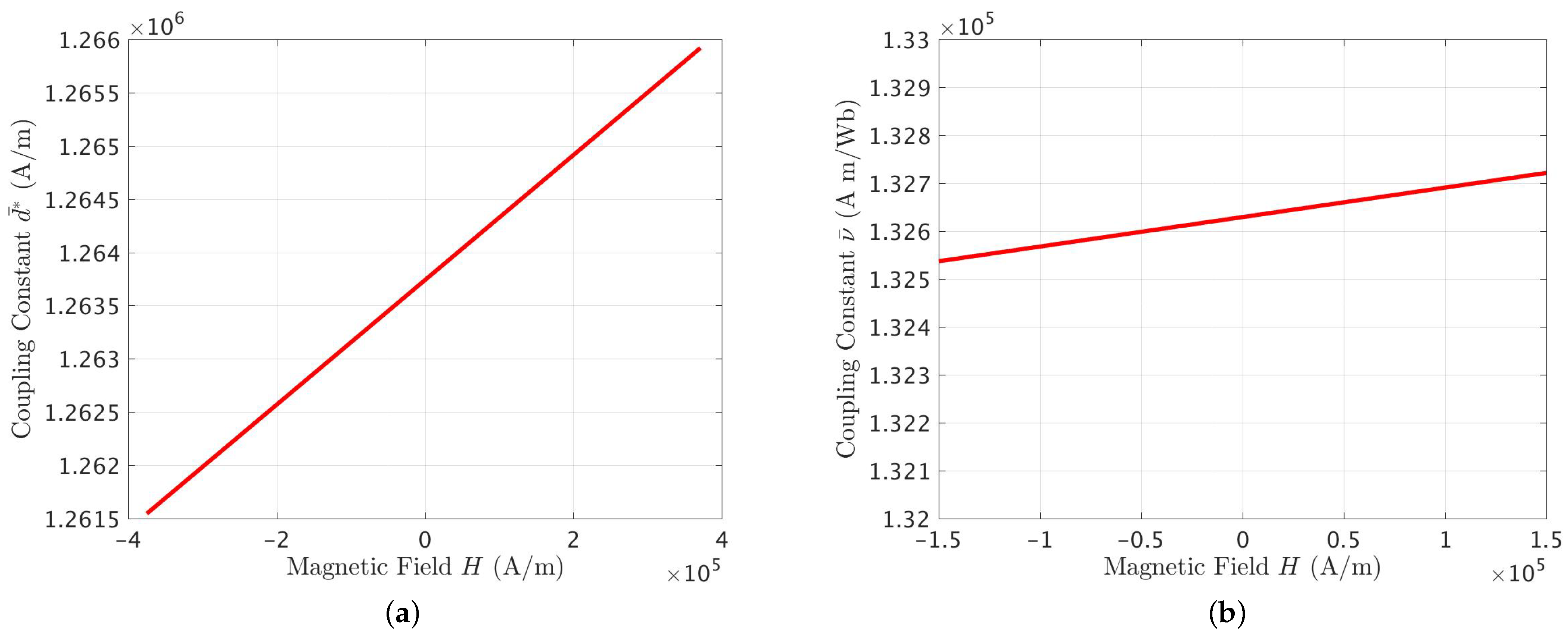
We point out here that the flexural rigidity term
in Equation (
20) is given by
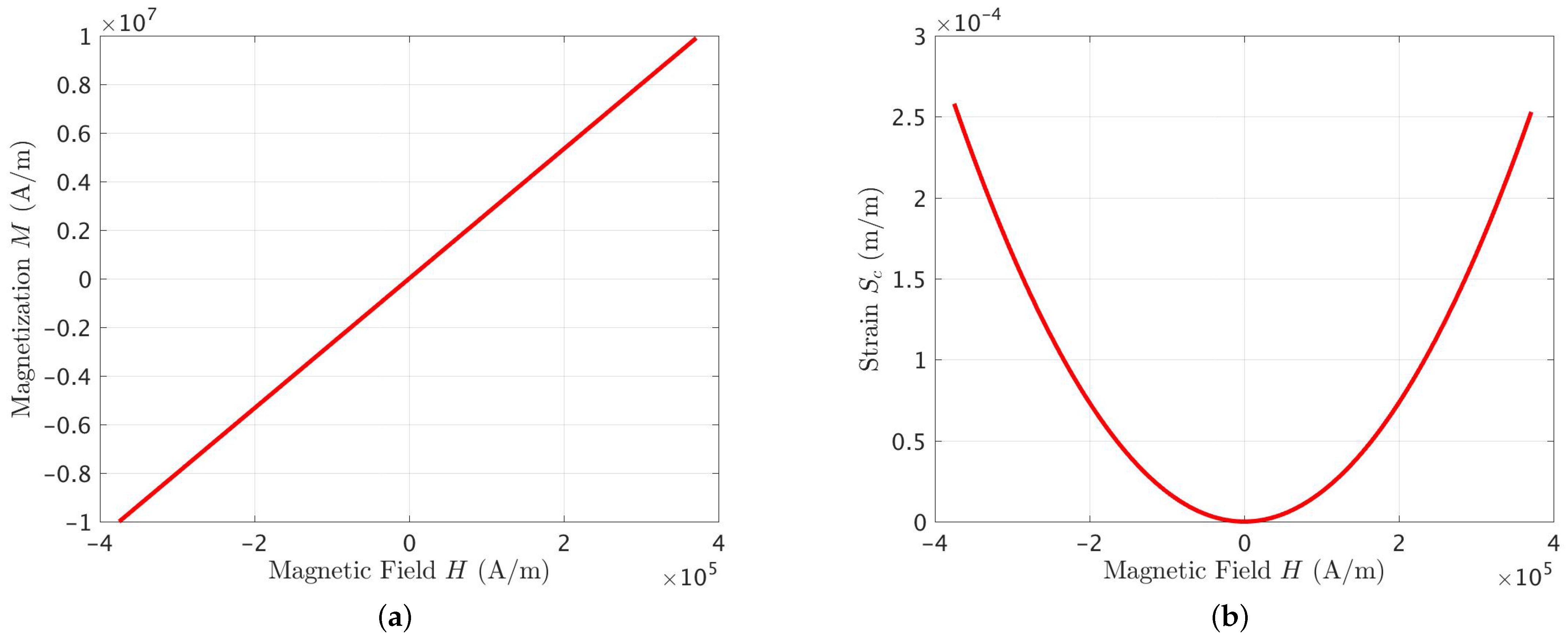
The magnetic flux density
is further related to the deflection
through
It is noted next that the voltage
produced across the coil wound around the Galfenol actuators is related to the magnetic flux density
according to
We assume that
(which includes changes due to flowing current) remains approximately constant during the oscillation for small oscillations and for a long coil of conductors over a strip. Therefore, its spatial and temporal derivates are approximated to zero. Then,
We use this approximation in Equations (
27) and (
30). From Equation (
30),
Then, if the coil on each strip spans from
to
, we find that the voltage difference between the two terminals of the coil is
Equation (
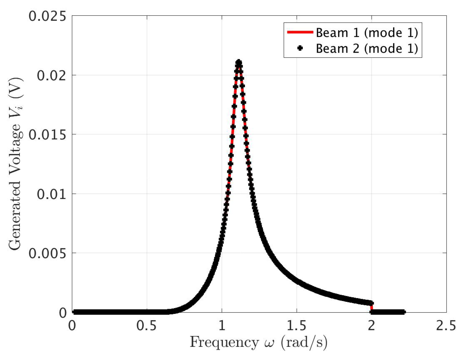
33) provides the voltage that would be available for use during the oscillation. Since Equation (
27) uses oscillation components in the vertical direction, substitution for
as expressed in Equation (
31) implies
Equations (
26) and (
34) describe the overall oscillation dynamics, with the waves imparting a predominantly heave oscillation on the buoy and the buoy acceleration then driving the beam deflections. Each of the Galfenol strips attached to the beams respond with a voltage difference between two ends of a conductor coil wound around it, as described by Equation (
33). The beam oscillations are consistent with the boundary conditions in Equation (
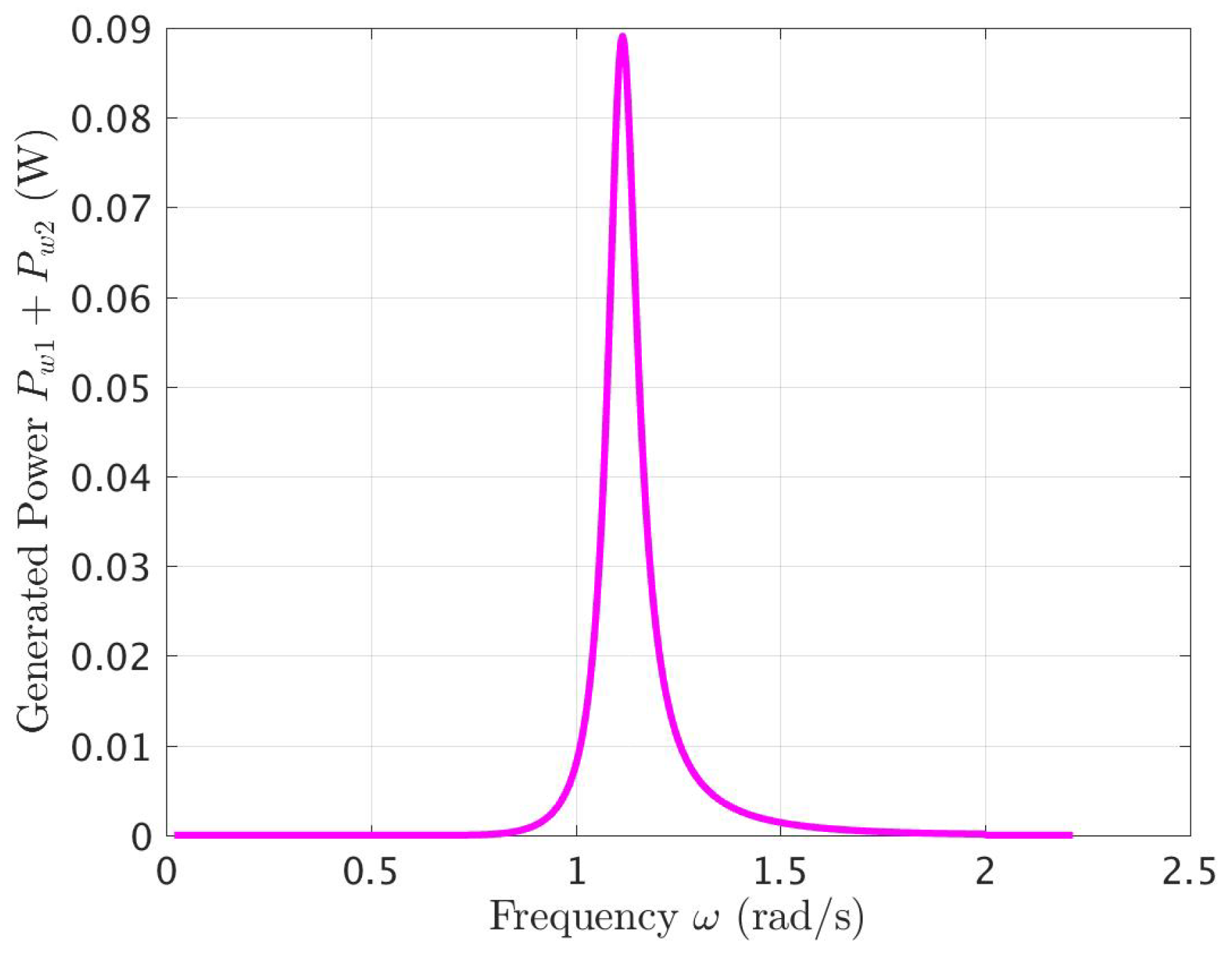
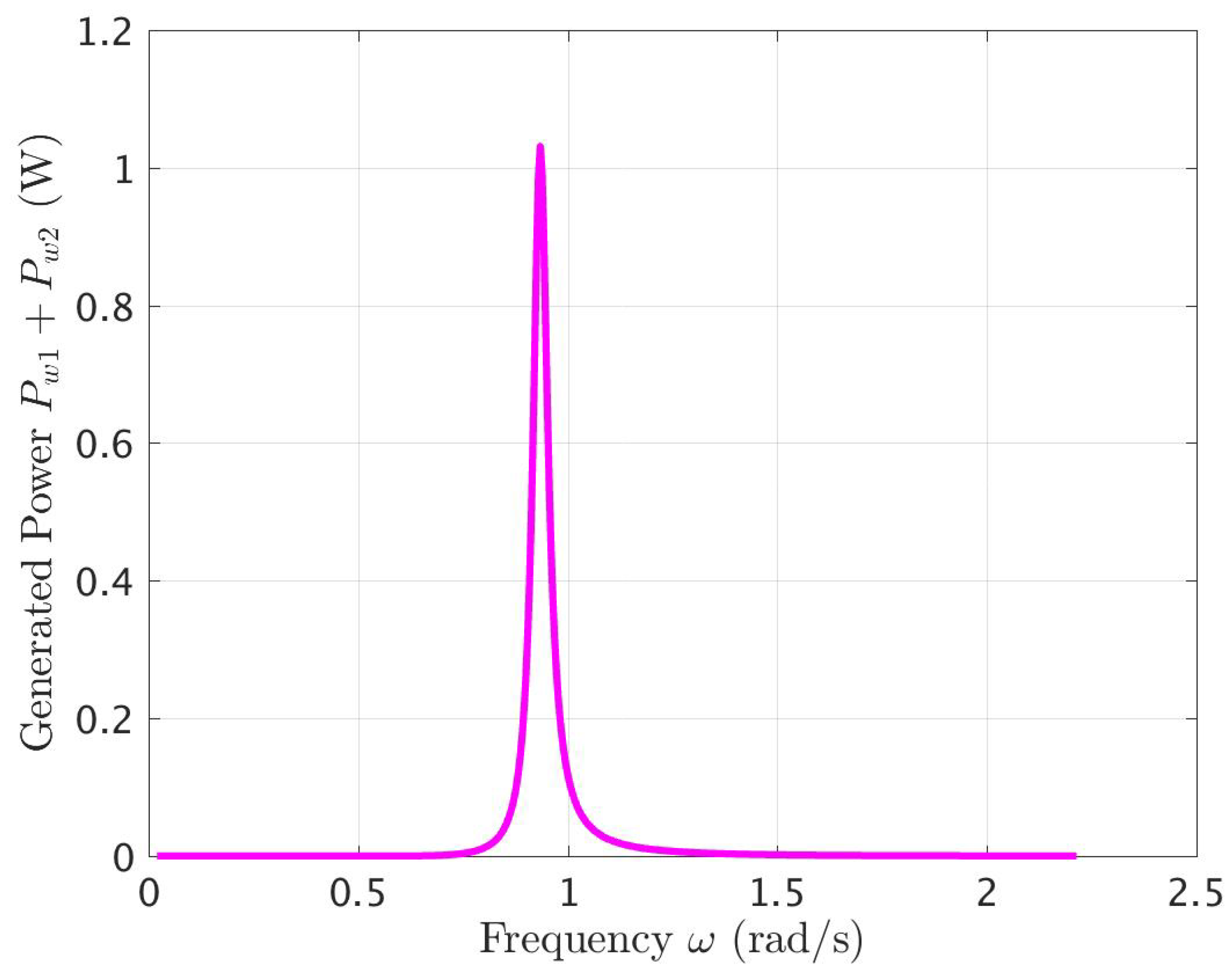
20). With a load resistor
connected across the conductor coil in a simple implementation, the power dissipated by it would be
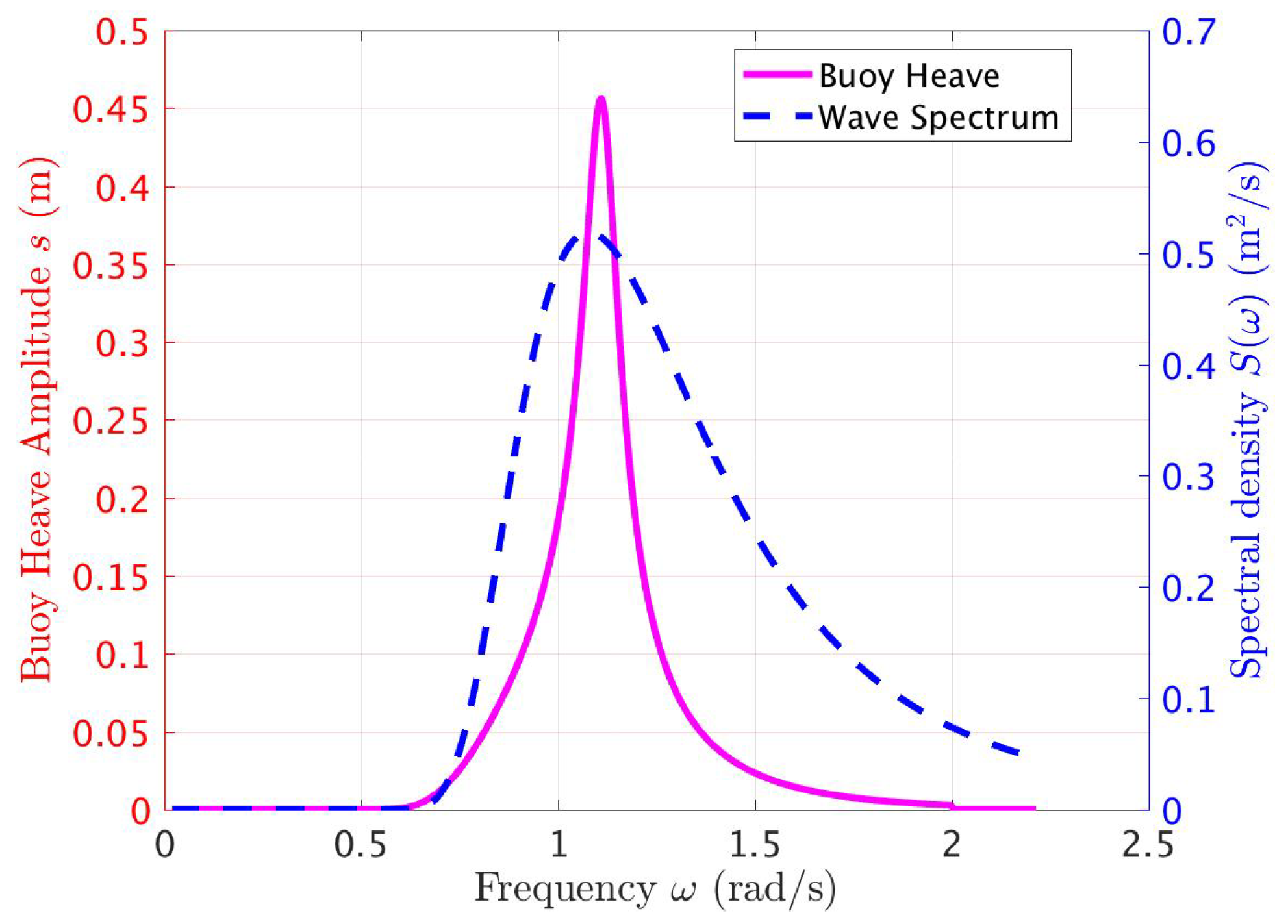
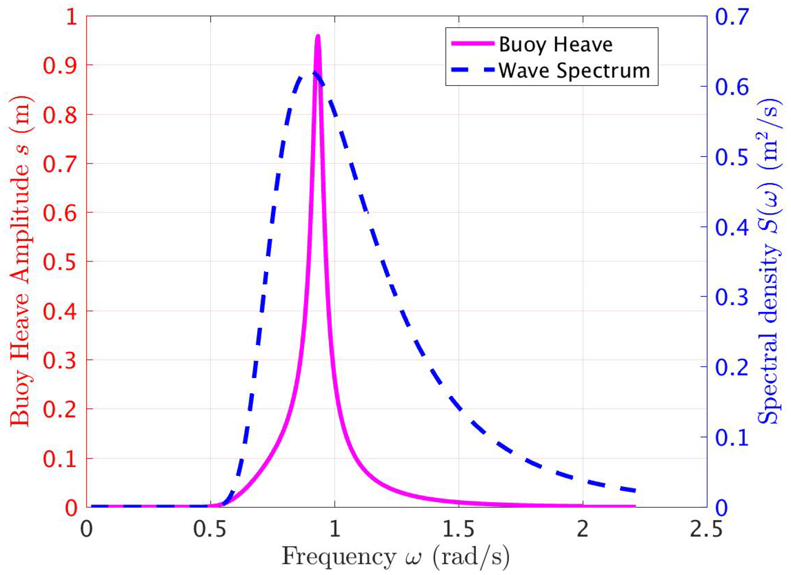
Buoy displacement and beam deflections can be evaluated when the wave-applied exciting force on the body is known. In this work, the time series were obtained for chosen irregular wave conditions, assuming long-crested Pierson–Moskowitz spectra. The spectral density was computed knowing the significant wave height and energy period , after which a wave elevation time series could be computed assuming superposition of a large number of frequencies (in this work, for most calculations) with the phase angles provided by a random number generator.
It is relatively straightforward to solve Equations (
26) and (
34) as a system by expanding the deflection
into its natural modes or eigenfunctions
as determined by the boundary conditions (
20). Thus, letting
where
are the time-dependent modal oscillations, and
We note that the modes
are mutually orthogonal. Expanding
in Equation (
34) for each beam into its eigenfunctions, multiplying both sides by
and integrating from 0 to
L, and utilizing the orthogonality property of the
nth eigenfunction
, we arrive at the following ordinary differential equations for each modal displacement
. This process results in the following system of equations.
This formulation allows
N to be a suitably large number. In this application, the source of excitation is surface waves, whose action is mostly confined to the frequency range
Hz, which corresponds to a wave period range of
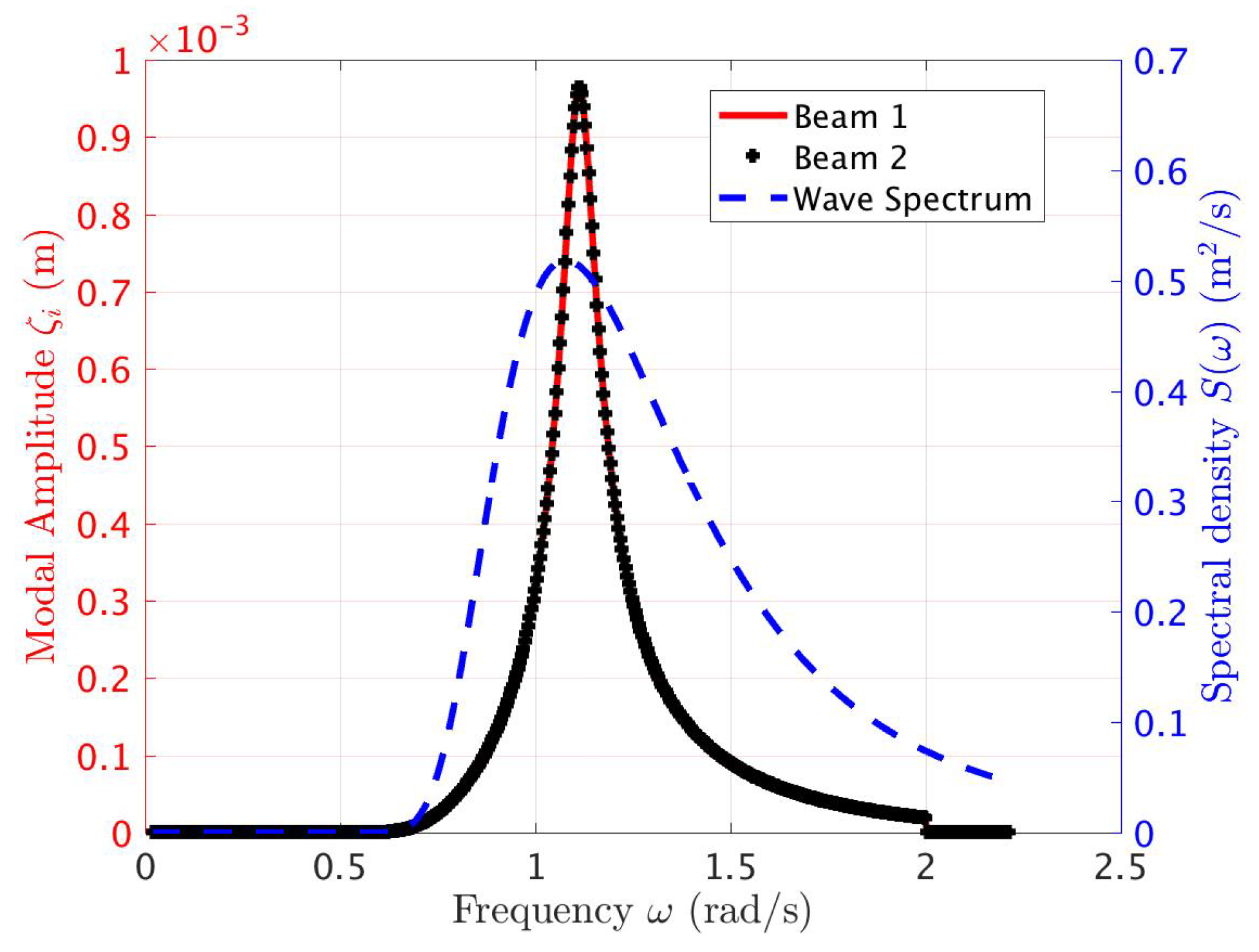
s. In light of this, it is argued that only the fundamental flexural modes of the present beams would be responsive to oscillations in the practical surface wave frequency range. We therefore just include the fundamental modes, so that
. Retaining just the first oscillation modes for the beams and taking the Fourier transforms of both sides of each remaining equation,
Here,
,
, and
are all complex-valued. The exciting force
, frequency-dependent added mass
, and the radiation damping
, etc., can be evaluated for a given geometry, using a numerical solver for a boundary-element type approximation. Equation (
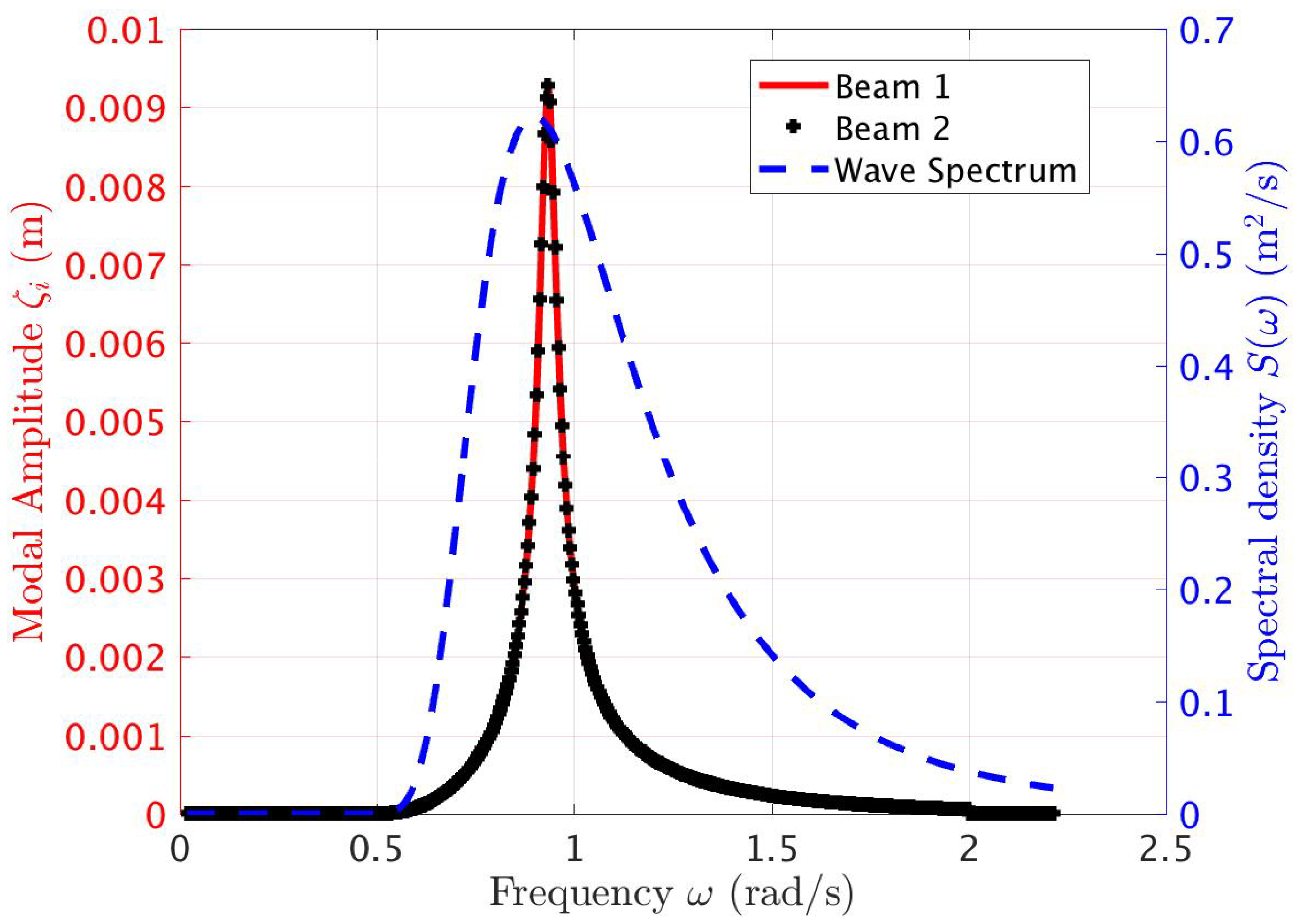
40) thus represent a system of algebraic equations which yields frequency-domain solutions for
,
, and
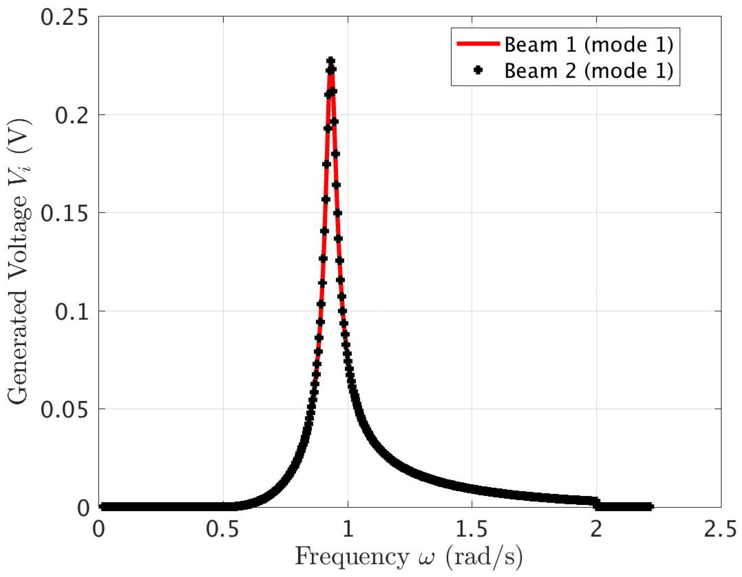
. The voltage across the conductor coil can then be determined and the power converted can be computed knowing the load resistor (or equivalent resistance in a load circuit being driven by the power take-off).
2.2.3. Beams Loosely Held within Deck Supports
In this case, the large clearance between the beams and the deck supports allows beam rotation about the points where they rest on the keel. As the buoy oscillates, it excites rigid body rotations of the beams that repeatedly are interrupted by impacts with the deck-support inner edges. Each impact acts as an impulsive load causing flexural vibrations over a range of natural modes. We expect that repeated excitation of some of the flexural natural modes may enhance power conversion beyond what is available through the fundamental-mode flexural vibration mode examined above. The dynamics of the overall system with this additional feature are modeled as described below.
In addition to the three main variables,
,
, and
above, there are now variables
and
that represent the rigid-body rotations of the beam about the rest-angle
, which is set to be the same for each beam, and each beam has a length
L. In this case, the beam end-masses also play an important role in the overall response. Further, in addition to the buoy exciting force
, there are now impact forces that act on the beams each time they collide with the inner periphery of their respective deck openings. The total kinetic energy of the system can be expressed as the sum of the following:
The potential energy of the system is the sum of
Assuming the rigid-body rotations of the beams
to be small, the boundary conditions of Equation (
20) are assumed to continue to be valid for this case too. The Lagrangian for this case is expressed as
Here,
and
. The external forces acting on the buoy in this case are the same as for the previous case. However, each impact causes an impulsive force to act on the beams that needs to be accounted for. Using Lagrange’s equations as outlined in Equation (
23) and assuming two beams, we arrive at the set of equations that describe the overall dynamics, starting with
for the buoy heave. Here,
includes the exciting force in heave on the buoy due to waves and the radiation force as in Equation (
26) above. The additional force
here is the force generated each time a beam impacts its support during its oscillation. An expression for this force is given following the remaining equations of motion. For the rigid-body rotation
of each beam, we have (assuming that
,
)
Next, for the flexural oscillation of each of the beams, we have
The impact force occurs each time the oscillating beam strikes the loose support, or at each
when
is the length of the short span of the beam (recall that a length
overhangs the support and that
). The magnitude of
can be expressed as
The equivalent mass of the beam
can be derived, for the fundamental oscillation mode, as
Once again, expanding the beam flexural oscillation into its eigenfunctions
as in Equation (
36) and for the moment, retaining just the fundamental mode, we arrive at the following system of equations. For buoy heave
, we have
Here,
and
are as defined above, including also
and
is given by Equation (
48), occurring at each
when the condition (
47) is satisfied. The equation of motion for
becomes
Finally, the flexural mode
is described by
In the results discussed here, a reduced version of the model in Equations (
50)–(
53) was tested, for quicker indications of the benefit of the proposed loose-fitting arrangement. The successive impacts were modeled using a series of Dirac delta function in the time-domain, and it was assumed that the impact-generated flexural oscillations decayed rapidly. In the frequency domain, the overall effect of successive impacts was approximated using the force
denotes the peak frequency in a spectrum. In the present calculations, the displacement of the beam relative to the buoy was assumed to be in phase for
, and opposite in phase for
.
denotes the wave-applied exciting force at the peak frequency
.


