1. Introduction
Hybrid active power filters (HAPFs) are a widely discussed type of equipment used for reactive and harmonic compensation [
1,
2]. When an active power filter (APF) is connected in series with a shunt passive filter it is possible to reduce the APF rating and improve the passive filter tuning, since the APF is able to electronically change the passive filter impedance. In [
3], the concept of active impedance is extended and the passive filter replaced by a capacitor bank. The APF is controlled as a smart impedance to compensate reactive power and harmonics. This HAPF topology is a reliable and cost-effective solution as it eliminates the need for an inductor and can be applied to an existing and operational capacitor bank.
This particular HAPF has been studied for power quality improvement of a single phase low voltage microgrid [
4], for reactive power compensation [
5] and to compensate both harmonic and reactive power using a multilevel converter topology [
6]. The reactive power compensation strategies require a fast response from the equipment in order to properly compensate for dynamic loads, such as in welding, arc furnaces, and wind generation, among others. In [
5,
6], this requirement is fulfilled by controlling the HAPF with finite control set model predictive control (FCS-MPC).
In fact, the application of FCS-MPC for power electronics converters has been studied for several years, due, specifically, to its fast dynamic response and its ability to consider systems’ nonlinearities and constraints [
7]. However, the FCS-MPC depends on the model parameters to select the control action applied to the system. Thus, parameter mismatches have an effect on the prediction of the state variables. This can result in inadequate cost function evaluation and, consequently, incorrect determination of the switching state. Which, in turn, may increase the THD and the steady-state error or even lead to instability in the system.
Due to the FCS-MPC nonlinear characteristic, it is not trivial to evaluate the effects of parameter uncertainties. The most common way to evaluate the system behavior against parameter mismatch is empirical, by analyzing the effects of these variations in the controlled current throughout several scenarios. In [
8], the authors take a mathematical approach to evaluating the prediction errors on an L-Filtered converter and conclude that variations in the series resistance are related to steady-state errors, while inductance mismatches cause an increase in the output current ripple, which is responsible for a higher THD. An expansion of this same analysis was produced in [
9,
10]. In these studies, the authors also considered the errors related to the model discretization and the sampling. Furthermore, a compensation method was formulated and tested in a laboratory setup.
Recently, solutions for parameter mismatch based on model-free predictive control approaches have also been investigated for L-filtered converters [
11,
12,
13]. In [
11] a neural predictor is integrated with a data-driven technique to predict unknown nonlinear system dynamics, model variations, and environment changes. In [
12], the proposal was to eliminate the system model using a first-order auto-regressive model with exogenous input (ARX), and the parameters were estimated using a recursive least square (RLS) algorithm. Following this, in [
13] the RLS algorithm is improved by using a dynamic-forgetting factor-based bias. Both techniques present a robust response to parameter mismatch. However, all proposals require a deep change in the control algorithm structure.
On the other hand, when FCS-MPC is applied to control an LCL-Filtered converter, which is the case for the HAPF topology used in this work, the method is prone to instabilities due to the delay in the model caused by the capacitor. Furthermore, the presence of the capacitor influences the FCS-MPC capacity to anticipate resonances. According to [
14], these instabilities can be avoided without increasing the prediction horizon by defining a proper cost function. In such a case, the cost function can indirectly control the grid-side current by controlling the inverter-side current, or by simultaneously controlling the inverter-side current and capacitor voltage. These references are calculated from the grid-side current reference and the mathematical model of the system. As a consequence, besides the errors in the predicted state variables (model uncertainties), the inaccuracies in parameters can also influence the calculation of the control references, which results in considerable deviations in the equipment’s operating point.
Due to the increase in the complexity of FCS-MPC in LCL-Filtered converters, research into parameter estimation techniques is quite recent and a wide range of investigation is still lacking. To the best of the authors’ knowledge, the main papers that address these methods can be categorized, according to the purpose of the estimation algorithm, into the following: estimation algorithms to correct the FCS-MPC model uncertainties [
15,
16,
17] and estimation algorithms to correct FCS-MPC control references uncertainties [
18].
Regarding the correction of uncertainties in the model, in [
15] the authors propose an adaptive gradient descent optimization method to fulfil this requirement. The results have higher accuracy and faster dynamic response when compared to a traditional state-feedback parameter identification method. A similar proposal is evaluated in [
16], but the authors utilize a moth–flame-optimization method. Finally, a model-free predictive control is proposed in [
17]. In this paper, the concept of [
12] is extended, and the RLS estimation algorithm is used to fit the parameters of a high order ARX model. However, in all of these papers a significant change in the FCS-MPC original structure is required, increasing the complexity of the control algorithms.
In contrast, the correction of uncertainties in the control references is addressed in [
18]. The authors utilize a grid voltage observer and a Luenberger observer to estimate the grid voltage, the capacitor voltage, the inverter-side current and the grid-side current. The grid voltage observer is used to generate the reference of the grid-side current, which is used in the FCS-MPC cost function. The proposal eliminates the need for several sensors and only the grid-side current is measured. The results show satisfactory performance for both steady state and dynamic response.
To summarize, the revised papers solve the problem of parameter uncertainties with estimation methods (such as state observers), or by modifying the structure of the FCS-MPC (such as model-free predictive proposals). They focus on L-filtered converters or LCL-filtered grid-connected converters. This paper, on the other hand, aimed to investigate parameter uncertainties of a Hybrid Active Power Filter, and to solve this problem so as to increase the robustness of this particular equipment, providing accurate reactive power compensation even with variations in the HAPF passive elements. Although the HAPF has the same mathematical model for the FCS-MPC prediction stage, its topology is different. The active part of the equipment is not connected to the point of common coupling (PCC). Thus, the output voltage of the LCL-Filter fluctuates between the grid voltage and the capacitor bank voltage. As a consequence, the equations for the control references calculation are strongly dependent on the capacitor bank reactance [
5].
In order to solve the problems related to parameter uncertainties in the control references calculation, this paper proposes a new method to estimate the capacitor bank reactance in the HAPF. The main contributions of this study include the following:
- 1.
The use of the weights of an adaptive notch filter (ANF) and the mathematical model of the system to estimate the capacitor bank reactance;
- 2.
No extra estimator is needed, since these ANFs are already used by the control algorithm to take the state variables to the dq coordinate system, as a substitute for the synchronous reference frame (SRF);
- 3.
The online estimation provides a way for the equipment to keep its operation in the case of a fault in a capacitive cell from the equipment’s capacitor bank.
As previously discussed, the analysis of the parameter uncertainties on the FCS-MPC prediction stage are not be considered here. In addition, the cost-function definition and the FCS-MPC control itself have been already discussed in [
5]. The focus of this paper is the application of the proposed online estimation technique to avoid deviations in the equipment operating point related to ill-calculated references. The method is implemented in a 7.5-kVA single-phase HAPF prototype in order to prove the effectiveness of the algorithm.
This paper is organized as follows:
Section 2 explains the ANF structure used to obtain the control references and the parameter estimates; the HAPF topology and the main control strategy are both presented in
Section 3;
Section 4 describes the proposed method of parameter estimation; the results obtained in a laboratory setup are presented in
Section 5 and
Section 6 provides the conclusions.
2. Adaptive Notch Filter
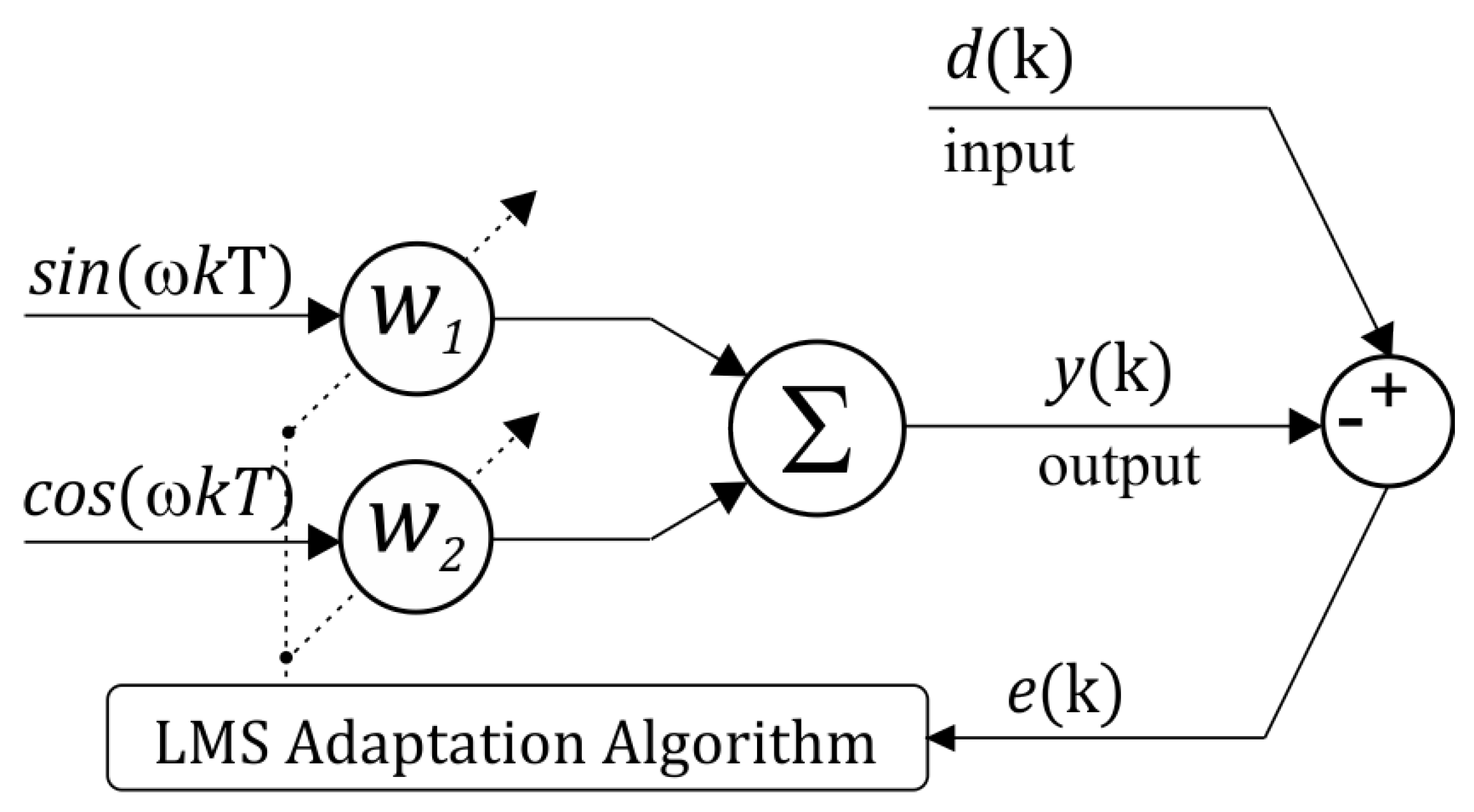
The ANF structure, presented in
Figure 1, was first introduced in [
19] for noise canceling, but, due to its characteristics, it has been applied for several different purposes in the field of electrical engineering, such as reactive power and harmonics detection and compensation [
20] and power calculations [
21], among others. The main advantages of this ANF are the easy bandwidth control and adaptive tracking of the fundamental frequency component of the signal.
The input signal (
) is assumed to be any kind of signal, or combination of signals, corrupted by noise. The input references are a pure sine and cosine wave with fundamental frequency
. The output signal (
) is a linear combination of the reference signals and the adaptive weights (
and
). The error (
) is used in the Least Mean Square (LMS) algorithm for adaptation. The operation of the LMS algorithm for updating the weights is given by:
where,
is the step-size value and determines the bandwidth (
) and the convergence rate of the algorithm and
T is the sampling period. For this structure, it is possible to assure stability for all values of the step size in the range of
[
19].
This ANF has only two coefficients. Therefore, its computational complexity is relatively small when compared to other structures [
22]. When applied to the extraction of electrical signal characteristics, such as voltage and current, the sine and cosine are provided by a PLL synchronized with a reference voltage. In this study, all ANFs were synchronized with the source voltage. Thus, the objective of filtering was to guarantee that
tracks the amplitude and phase of the component with frequency
from the signal
. As a consequence, the weights
and
carry relevant information about the fundamental component.
So, assuming the output signal is a pure sine wave, with amplitude
A, phase
, and frequency
, it is represented as:
Using the trigonometric identities, we can also represent (
3) as:
On the other hand, as shown in
Figure 1, the ANF output signal is given by:
Comparing (
4) and (
5), we obtain:
An analogy can be made between the ANF weights and the SRF direct and quadrature components (
dq components). However, the ANF has better dynamic response and a shorter processing time than the SRF, as explained in [
21].
In this paper, the presented ANF structure is used to extract the load reactive current component, which is applied to calculate the control references for reactive power compensation. The main contribution of this study is also the use of this same ANF structure to estimate the HAPF parameters by means of the ANF weights and the system mathematical model.
3. Hybrid Active Power Filter Control with FCS-MPC
The operating principle of the HAPF topology used in this work was extensively discussed in [
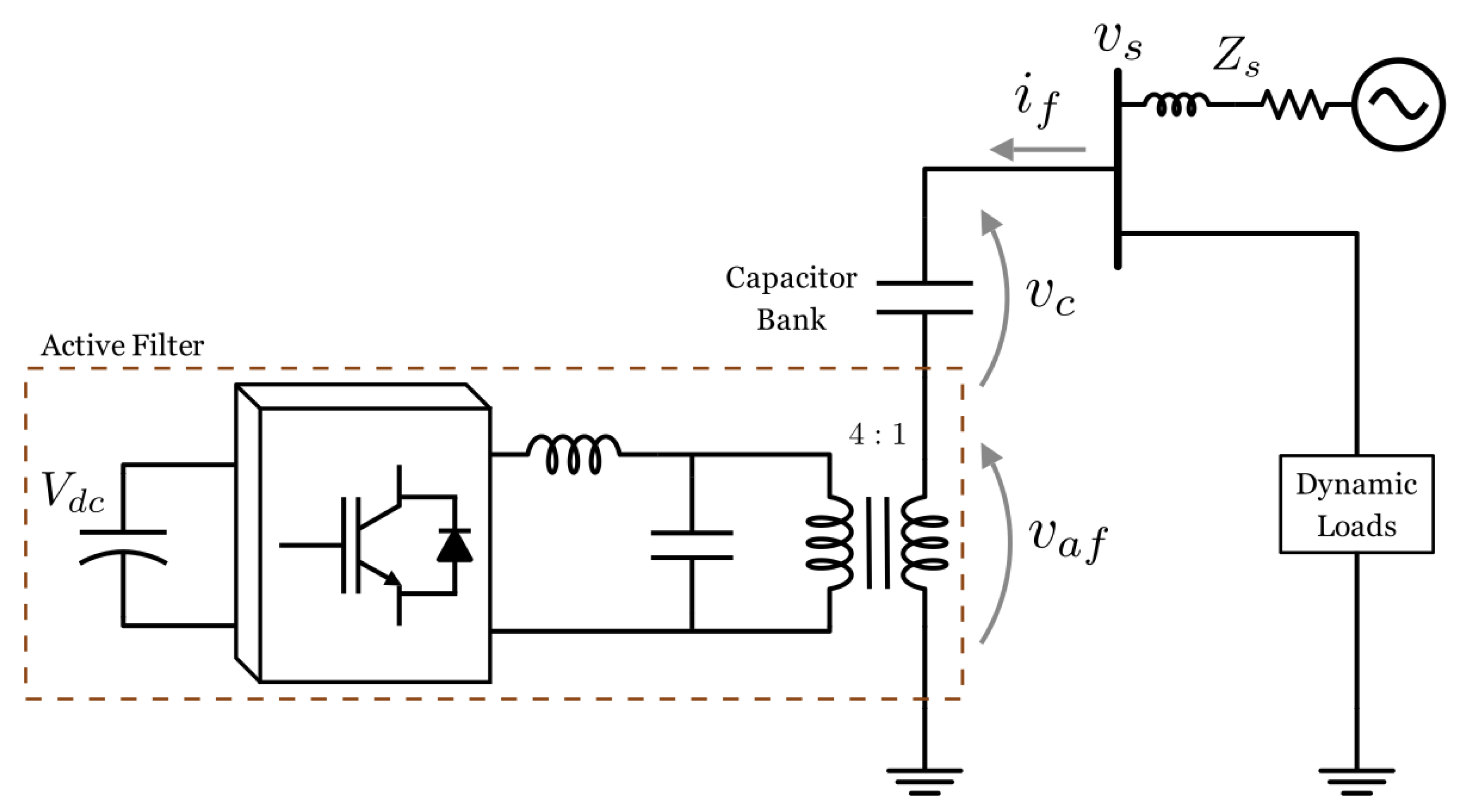
3]. In spite of the equipment’s capability to compensate for reactive power and harmonic frequencies, in this work only the reactive power control loop is explored. This equipment can be applied to compensate the reactive power of dynamic loads, such as arc furnaces, wind farms, fluctuating reactive loads, and welding operations, among others. The simplified diagram of the HAPF is shown in
Figure 2, where
,
,
and
are the active filter voltage, the capacitor bank voltage, the source voltage and the DC link voltage, respectively and
is the hybrid filter branch current, which is predominantly capacitive at the fundamental frequency due to the capacitor bank.
Proper control of the filter current () assures dynamic compensation of reactive power. In this HAPF topology, the control of is performed by applying the necessary voltage to , which, in turn, controls the voltage over the capacitor bank so that the reactive component of follows a given reference.
In [
5] the use of FCS-MPC was proposed to improve the HAPF transient response, as an alternative to classical controllers in the SRF. The FCS-MPC aims to minimize a cost function by evaluating the discrete model of the system only for the finite-set of possible switching states of the converter [
23]. The main aspects for successful implementation of FCS-MPC are proper system modeling and cost function definition, which are summarized in the next sections.
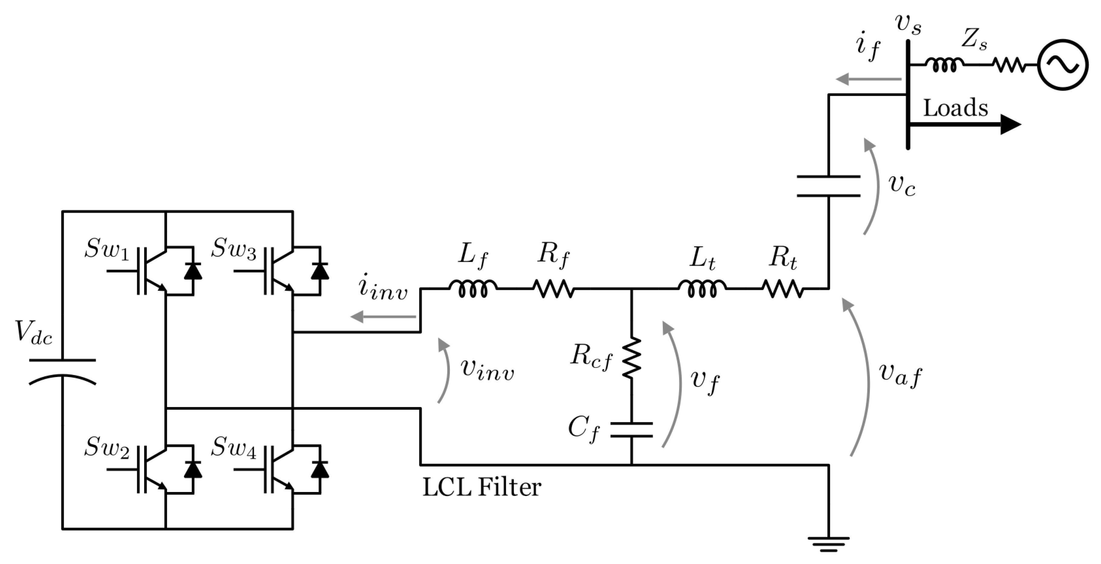
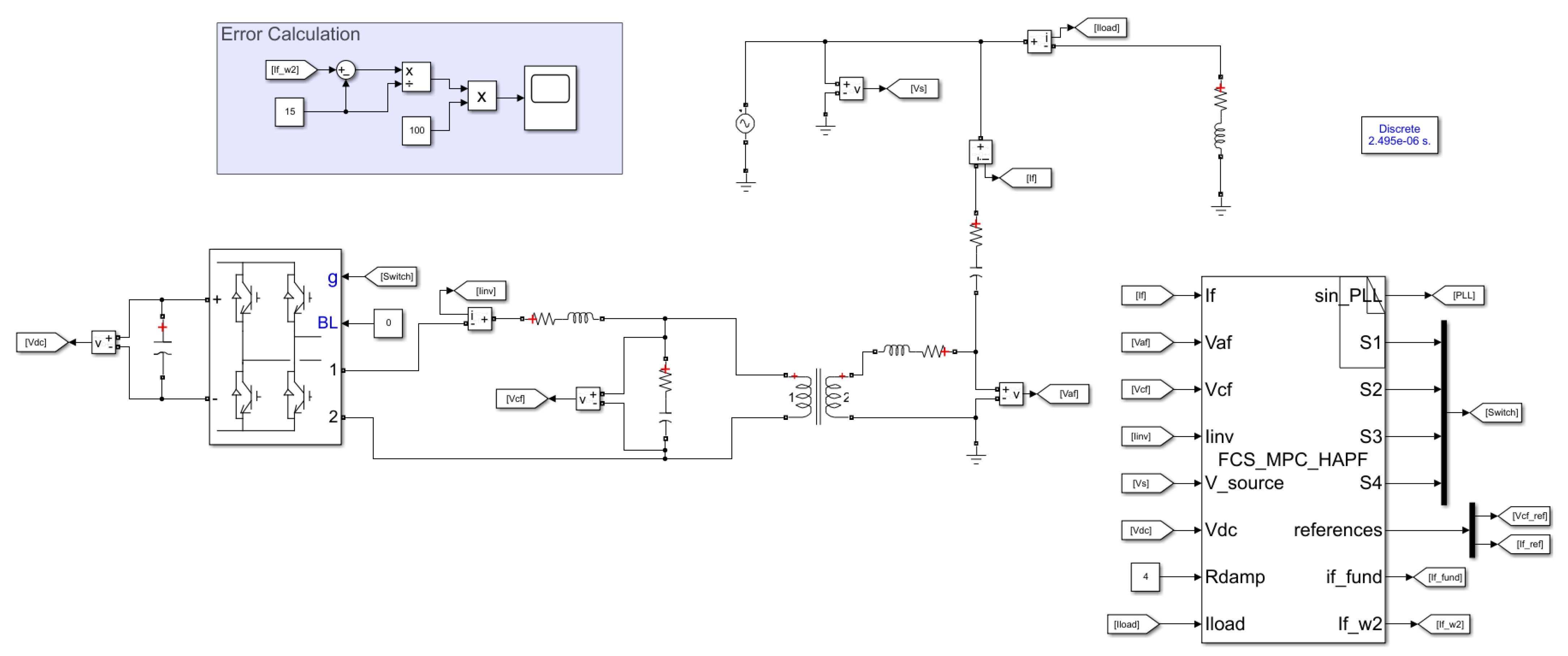
3.1. HAPF Modeling
In order to model the HAPF, its variables were considered in per-unit (
) values and the transformer was modeled by means of its series impedance, as detailed in [
5]. As a result, the complete circuit of the HAPF is presented in
Figure 3.
Note the following:
and
are the inverter filter inductance and its inner resistance;
and
are the filter parallel capacitance and its inner resistance;
and
are the short circuit transformer resistance and inductance, respectively. In addition,
and
are the inverter voltage and current,
is the filter capacitor voltage and
are the switching devices. Due to the coupling transformer, the
pu representation makes state–space modeling easier. The state–space model of the HAPF is described in [
5]:
where,
The discretization of the state–space model from (
9) is written as:
Where,
k is the sampling instant and
and
are the discrete forms of the matrices
and
shown in (
10). The system model discretization is realized by the forward Euler method and, since a high sampling frequency is used (40 kHz), it is possible to ignore higher order terms, which results in [
14]:
where
is the sampling period. The discrete HAPF model is used to predict the state variables for the next sampling instants. In this work, a single-phase H-Bridge converter was used. However, the concepts can be extended for three-phase and multilevel converters, as in [
6]. For single-phase inverters, the algorithm must consider four switching states (
), which results in the following voltage vectors:
,
,
and
.
3.2. Cost Function Definition
In LCL-Filtered converters, the direct control of
is not trivial and usually requires longer prediction horizons (
). The filter capacitor introduces a delay in the model equations, and, thus, the manipulated variable (
) is no longer related to the controlled variable (
) in the next sampling instant, as in L-Filter models [
24]. Aiming to avoid long prediction horizons and the consequent increase in processing time, the application of FCS-MPC with a multi-variable cost function was presented in [
14,
25]. According to this study, the application of a multi-variable cost function to control more than one of the LCL-Filter state variables is a simple way to assure stability and avoid resonances. So, here, the control of the inverter output current (
) guarantees the system’s stability, while the filter capacitor voltage (
) control is responsible for avoiding harmonics and resonances. As a result, the multi-variable cost function is given by:
where
and
are the cost function gains which define the control priorities,
and
are the reference and the predicted values of the inverter output current,
is the filter capacitor voltage reference, considering the resonance active damping, as shown in
Section 3.4 and
is the predicted value of the filter capacitor voltage, respectively. A prediction horizon of
was adopted. First, the state variables are estimated for the next sampling instant in order to compensate for the delay caused by the processing time, and, then, the cost function is evaluated for the predicted state variables two instants ahead [
26].
In a typical FCS-MPC application the cost function may also contain other terms that are designed to consider system nonlinearities, constraints or other secondary control objectives. Examples of these include the following: reduce common-mode voltages [
27], apply converter output current limitations [
28,
29], reduce thermal stress on semiconductor devices [
30], reduce losses by penalizing the number of semiconductor commutations [
15,
31], and control the converter switching frequency [
32], among others. However, since the objective of this paper was to demonstrate the effectiveness of the proposed parameter estimation technique, the cost function was kept as simple as possible and no constraints were considered.
3.3. Control References
The FCS-MPC with multi-variable cost function deals with the drawbacks of LCL-Filtered converter control. Nonetheless, since the control is based on the hybrid filter current reference (
), the control references for the capacitor filter voltage (
) and for the inverter current (
) must be obtained indirectly by the system model. In the following sections, a summary of the control references calculation is presented, and the detailed equations are presented in [
5].
3.3.1. Reference of Hybrid Filter Current ()
The reference current
controls the reactive power delivered by the HAPF and assures DC link voltage regulation. This current can be represented using the
dq axes:
The active current is controlled by the direct axis component (
), which is responsible for the DC link voltage regulation and is obtained by a PI controller. The reactive current is controlled by the quadrature component of the current (
), which is responsible for the reactive power control. The reactive current reference can be set manually for static operation of the equipment or, in the case of dynamic compensation of load reactive power, this reference is obtained through an ANF applied to the load current (
), which results in:
where,
is the output of the ANF, and
,
are its adaptive weights. Considering the result obtained in (
7), and the analogy to the SRF, the weight
is the quadrature, or reactive component, of the load current. Thus, the hybrid filter reactive current is controlled in such a way that
, ensuring the unit power factor in the source.
3.3.2. References of Filter Capacitor Voltage () and Inverter Output Current ()
As previously discussed, the state variables that are actually controlled are the filter capacitor voltage (
) and the inverter output current (
). The references for these variables are based on the HAPF current reference (
) and the system model. The system model is derived from the equivalent circuit, shown in
Figure 3. Using a phasor representation, the reference variables are calculated as:
where
R is the hybrid filter branch resistance-composed by the capacitor bank series resistance (
) and the transformer resistance (
) −
X is the equivalent reactance of the hybrid filter branch-composed by the inductive reactance of the transformer (
) and the capacitive reactance of the capacitor bank (
)− and
is the filter capacitor reactance. The filter capacitor series resistance is disregarded for the reference calculation. To proceed with the calculations it is assumed that:
As previously stated, the value of
is obtained through a PI controller and
is the coefficient from the ANF applied to the load current. Then, another ANF is applied to the source voltage, which provides the coefficients
and
used in the phasor representation of this variable. In addition,
and
can also be represented as:
where,
and
are the direct components of the capacitor voltage and inverter current references, and
and
are the quadrature components of the capacitor voltage and inverter current references, respectively. Finally, the time domain references,
and
, are obtained as:
It is noteworthy that this method uses the system model and one extra ANF to calculate the references for
and
. The overall control processing time is not significantly increased, and the need for long prediction horizons is avoided. In fact, in [
5,
14] the authors already demonstrated the effectiveness of using FCS-MPC with a multivariable cost function and estimated references. However, they highlighted that model inaccuracies could make this approach prone to current deviations from the set point. This can be realized by analyzing (
17), since the parameter values are directly related to the references being calculated, deviations in these values are translated into incorrect references, which are tracked by the FCS-MPC and cause the equipment to operate outside the desired point.
3.4. Resonance Damping Method
In order to dampen the resonances, and to block the circulation of harmonic currents due to source voltage distortion, a virtual resistance (
) is added to the system. The concept of virtual resistance in series with the output inductance for that purpose is not new [
33], having been adopted by several papers with FCS-MPC and other control algorithms [
14,
24]. To achieve such an effect, the hybrid filter branch current (
) is filtered by an ANF to eliminate its fundamental component, the same ANF structure from
Figure 1 is applied, and the hybrid filter harmonic content (
) is the error signal obtained. Then,
is multiplied by a virtual resistance (
) to generate a damping term to be added to the filter capacitor voltage in order to generate a new reference, as:
where
is the active term responsible for the source voltage harmonic damping.
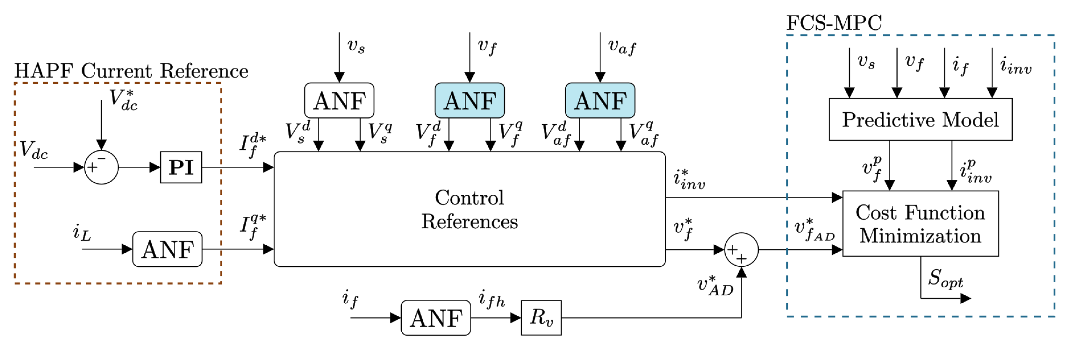
3.5. Summary of FCS-MPC Control Loop
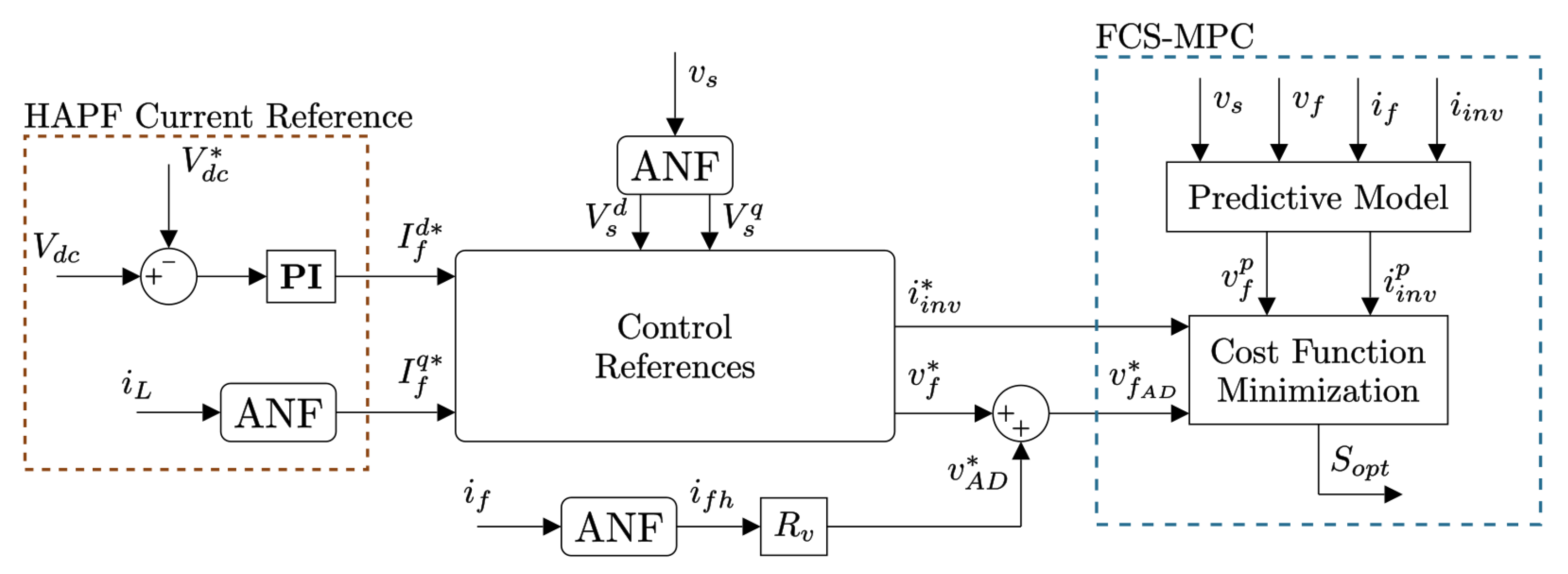
The block diagram of
Figure 4 summarizes the control strategy applied to the HAPF. The algorithm is divided into the following blocks: definition of the HAPF branch current reference (
); FCS-MPC references calculation (
and
); FCS-MPC control loop.
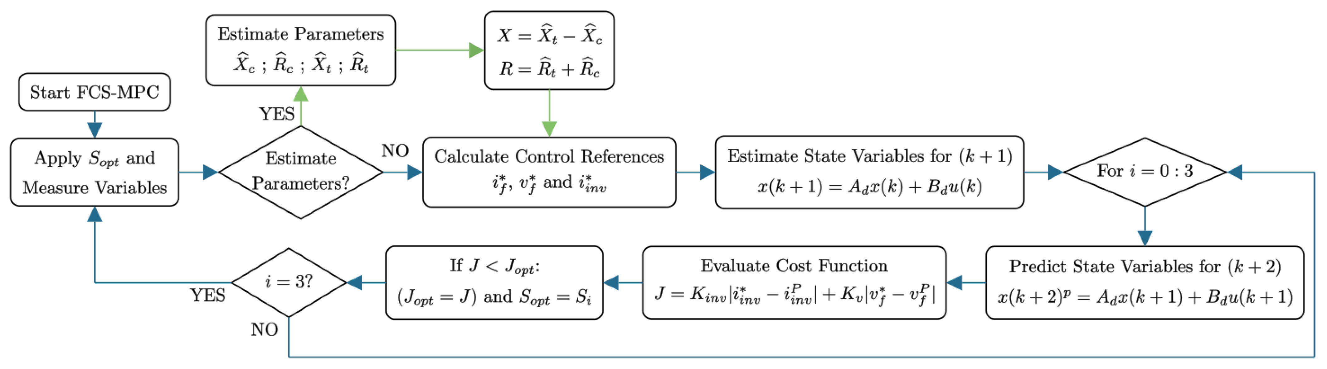
The control references are obtained according to the method described in
Section 3.3, and the FCS-MPC control loop follows the steps below:
- 1.
Estimate the system states for (
) from (
9), in order to compensate for the computation time delay;
- 2.
Predict the system states for (), considering all possible switching states;
- 3.
Evaluate the cost function based on the predicted variables and reference variables previously obtained;
- 4.
Define the optimum switching state () that minimizes the cost function, which is applied in the next sampling period.
In the following section, the influence of parameter mismatch on the control references calculation is discussed and a method to estimate the capacitor bank reactance is proposed.
5. Results
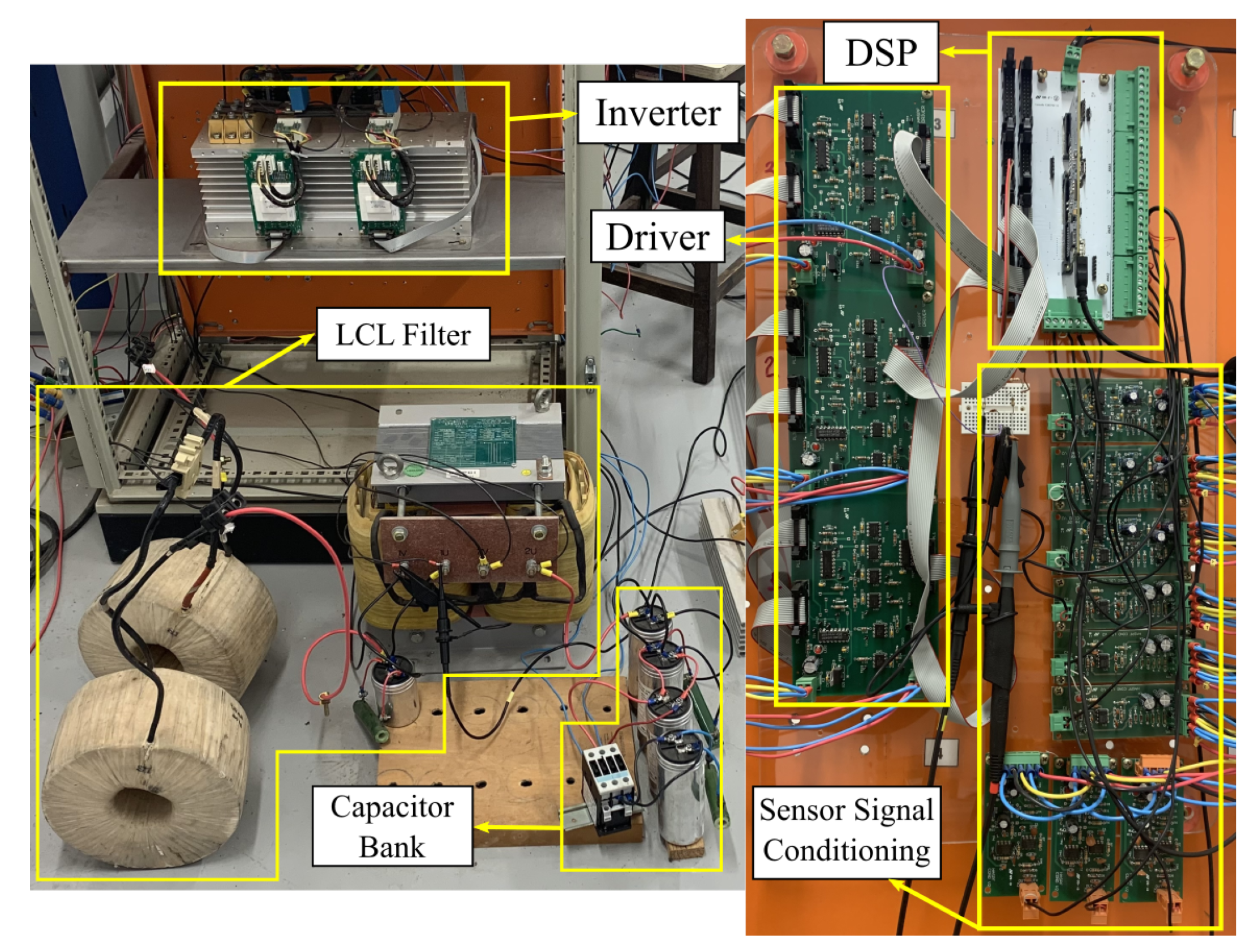
The proposed method for parameters estimation was tested in a laboratory setup assembled according to the diagram shown in
Figure 2. The system setup followed the one described in
Table 1 for the simulations and the hardware used to run the algorithm was a DSP TMS320F28379D. The HAPF laboratory setup is shown in
Figure 9.
In order to properly evaluate the algorithm response to variations in the capacitor bank reactance value, the setup was composed of 4 paralleled capacitors, one of which was connected through a contactor, which allowed the capacitor bank value to be changed during the equipment’s operation, simulating a fault in one of the capacitors. Each capacitor had a nominal value of F, which made for a total of F when all capacitors were connected and F when one of them was removed.
To test the algorithm’s response to multiple scenarios, the tests were divided into two: first, a fixed reactive power reference was provided to the FCS-MPC; and, in the second test, the HAPF compensated the reactive power from a load. In both tests the capacitor bank value was changed during the equipment’s operation. It is important to note that the capacitor bank value was set to F during the algorithm’s initialization. Therefore, this is the value considered by the reference generation algorithm when the parameter estimation is not activated, regardless of the number of capacitors connected to the capacitor bank.
5.1. Fixed Reactive Power
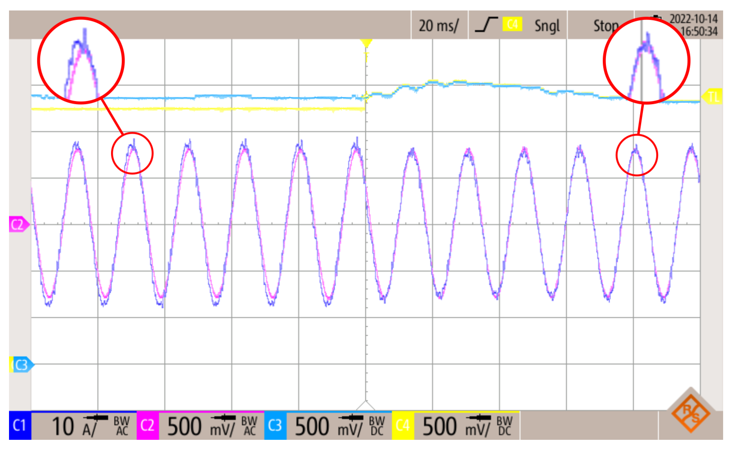
To visualize the algorithm’s capability to adjust the HAPF branch current to its reference,
Figure 10 shows the moment when the estimation algorithm is activated. The peak value for the HAPF reactive current reference (
) is set to 16 A, the oscilloscope channel 1 (Blue) shows the HAPF current, channel 2 (Pink) shows the current reference, channel 3 (Cyan) is the estimated capacitor bank capacitance and channel 4 (Yellow) is the capacitance value being used in the control reference calculation. A
F/V relation was used to plot the capacitance values from the filtered DSP PWM outputs.
Before the prediction algorithm was activated, the capacitance value used in the control reference calculations was the nominal F, shown in yellow. However, the real capacitance value estimated by the algorithm was around F. This created an error between the reference value and the actual HAPF current. Once the estimation algorithm was activated there was a little overshoot in the estimated value, due to the changes in the control references, but, after around cycles, the estimated values returned to the correct values. Nevertheless, the HAPF current followed the correct reference as soon as the estimated values began to be used in the reference calculations. After the activation of the estimation algorithm, some perceptible oscillations appeared in the estimated capacitance value. This occurred as a result of the ANF adaptation times, and ceased once the weights were fully adapted.
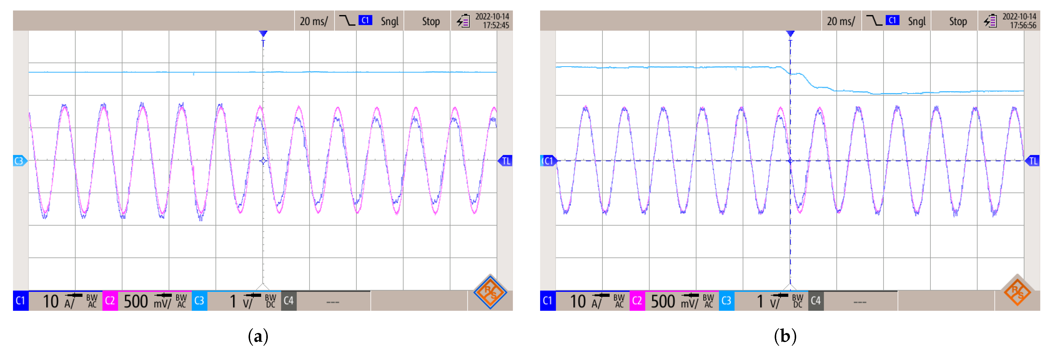
Figure 11 shows the HAPF current behavior when one of the capacitors is removed from the capacitor bank. In this figure, the cyan line indicates the capacitance value used by the control reference calculation. In
Figure 11a, the estimation algorithm was not activated, so the capacitance used in the control reference calculation kept its value of
F for the entire time, which created a considerable error between the HAPF current and its reference value.
Figure 11b shows the case where the online parameter estimation was activated. After the removal of one capacitor from the capacitor bank, its estimated capacitance changed from
F to
F. This guaranteed that the HAPF kept supplying the desired reference and the capacitance value adjustment was completed in around
fundamental cycles.
The result of
Figure 11b also demonstrates the estimated capacitance value behavior prior, during, and after a big variation in the capacitor bank value. As previously discussed, the oscillations in the estimated capacitance value, when the estimation algorithm was activated, (
Figure 10), disappeared when the ANFs’ weights were fully adapted. This was demonstrated by the estimated value prior to the capacitor bank variation, in
Figure 11b, which had no oscillations. When the capacitor was removed from the capacitor bank some oscillations were visible, due to the adaptation process of the ANFs’ weights, but, once again, these oscillations only occurred while the weights were being adapted.
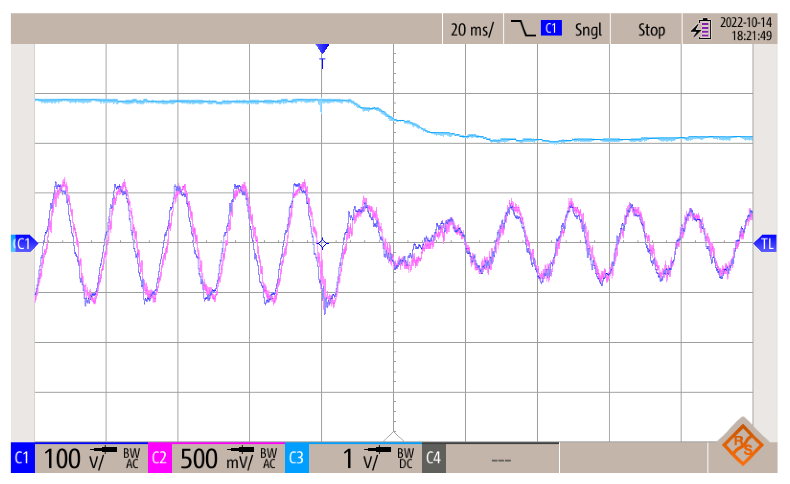
Another important variable to visualize is the filter capacitor voltage (
) when the capacitor bank value changed, which is shown in
Figure 12. Now, the oscilloscope channel 1 (Blue) shows the filter capacitor voltage, channel 2 (Pink) shows the filter capacitor voltage reference (
) and channel 3 (Cyan) still shows the capacitor bank capacitance used in the control reference calculation. As expected, when one capacitor was removed from the capacitor bank its total capacitance reduced, so, in order to keep supplying the same current, as already shown in
Figure 11b, the voltage across the capacitor bank had to be increased. This effect was achieved by reducing the voltage over the active part of the HAPF and, likewise, the filter capacitor voltage reference was reduced.
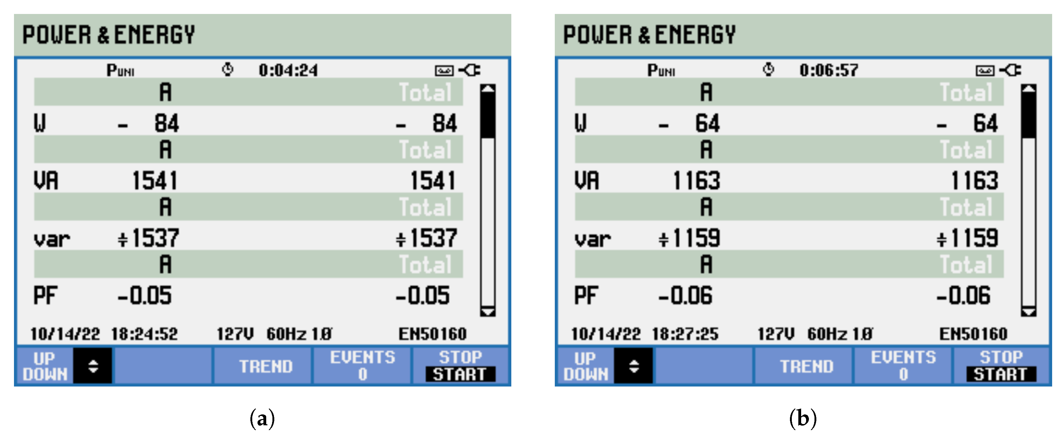
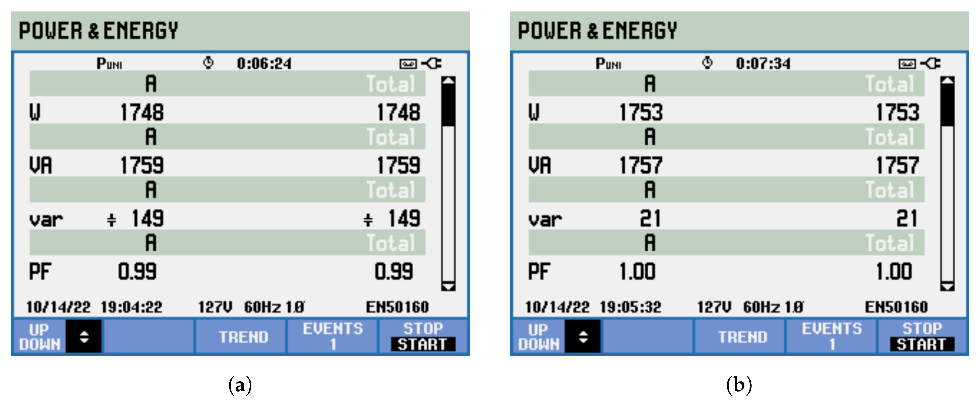
When a fixed reactive current reference was provided to the FCS-MPC algorithm the HAPF acted as a capacitor bank, supplying the desired reactive power. Before the application of the proposed algorithm for parameter estimation, the power supplied by the HAPF was measured for a configuration with four and three capacitors, respectively. In both measurements, the reactive current reference was kept at 16 A. The results are shown in
Figure 13.
The actual value that the HAPF must supply when
A should be around 1436 Var, depending on the source voltage level, but, as depicted in
Figure 13a, even when the capacitor bank was operating with its nominal value of
F, the reactive power measured was not the correct one, sitting around 1537 Var. This was due to variations in the real value of the capacitors and some source voltage fluctuations. When one capacitor was removed from the capacitor bank, the reactive power value moved even further away from the expected value, as shown in
Figure 13b.
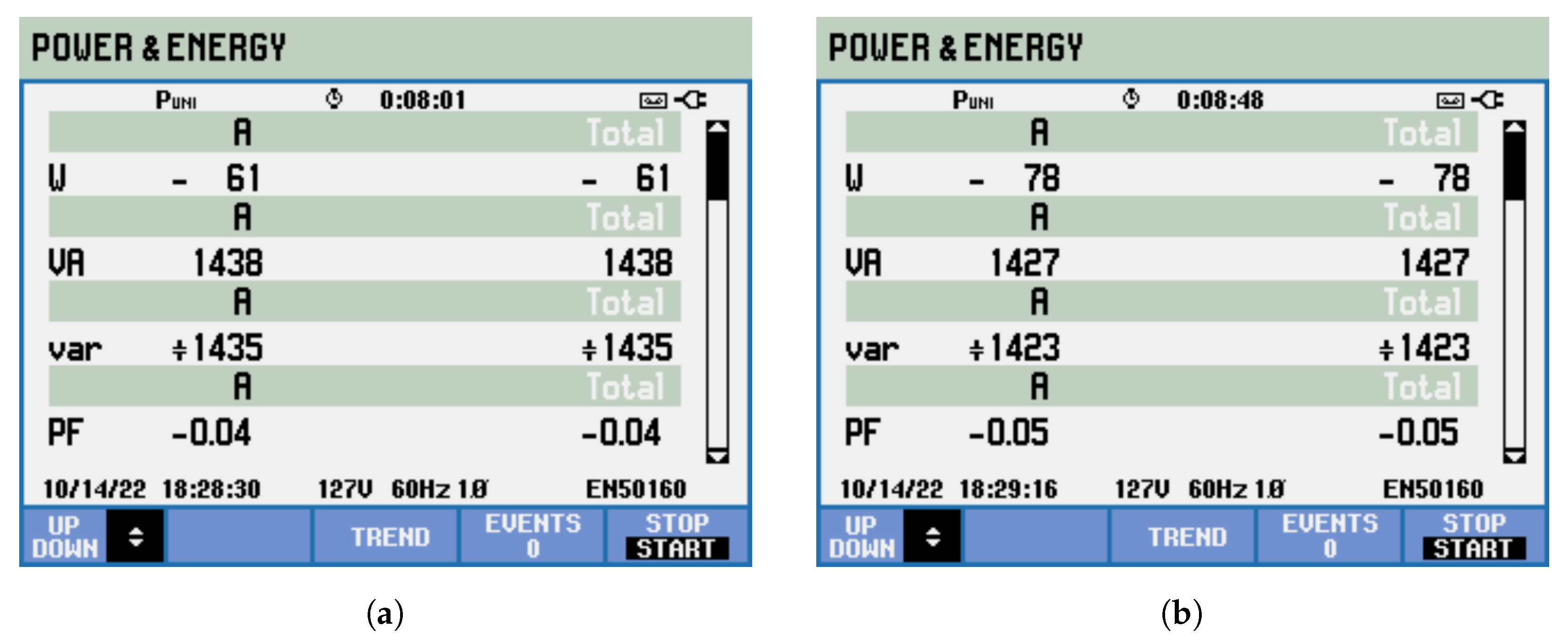
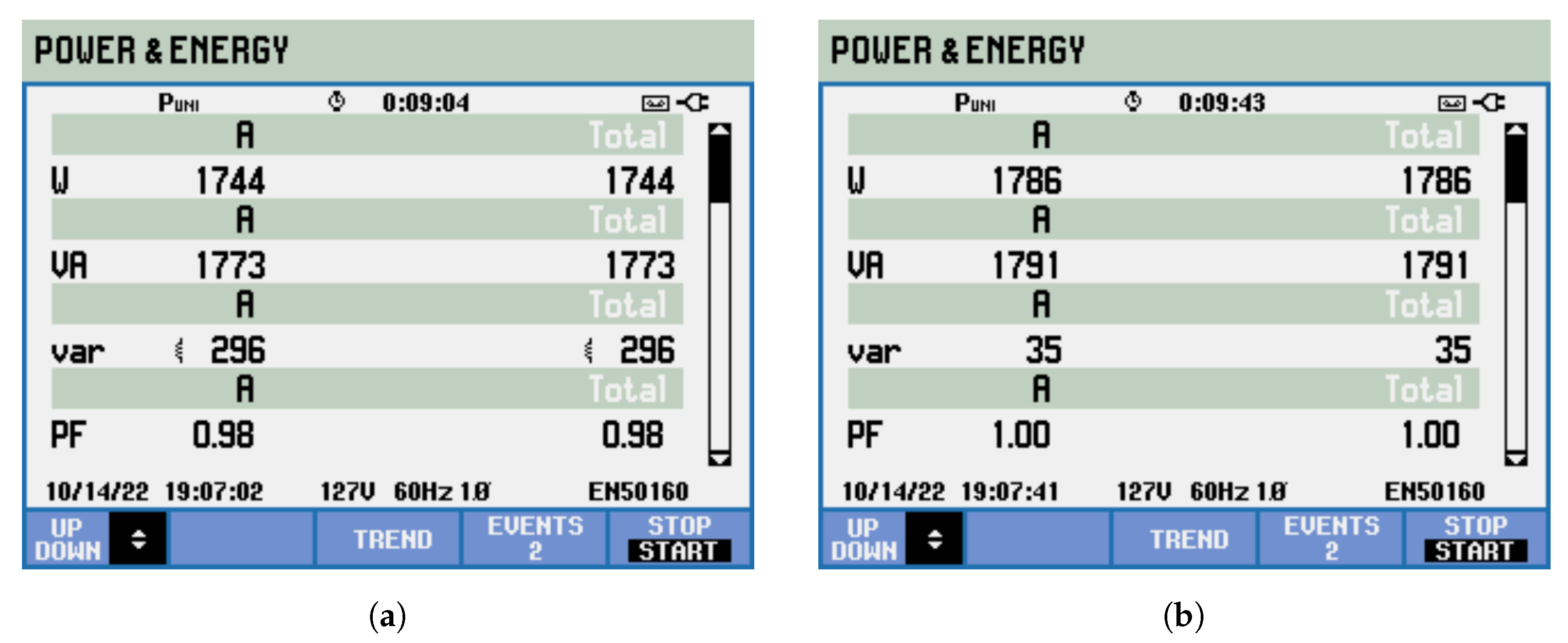
Once the online parameter estimation algorithm was activated, the reactive power supplied moved to a value closer to the expected one, as shown in
Figure 14.
Figure 14a shows the result for a capacitor bank with 4 capacitors. The equipment supplied 1435 Var, which was a value very close to the nominal. The small variation observed may be the result of a fluctuation in the source voltage value. When one capacitor was removed from the capacitor bank there was almost no change in the HAPF reactive power, as shown in
Figure 14b. This demonstrates the effectiveness of the proposed method.
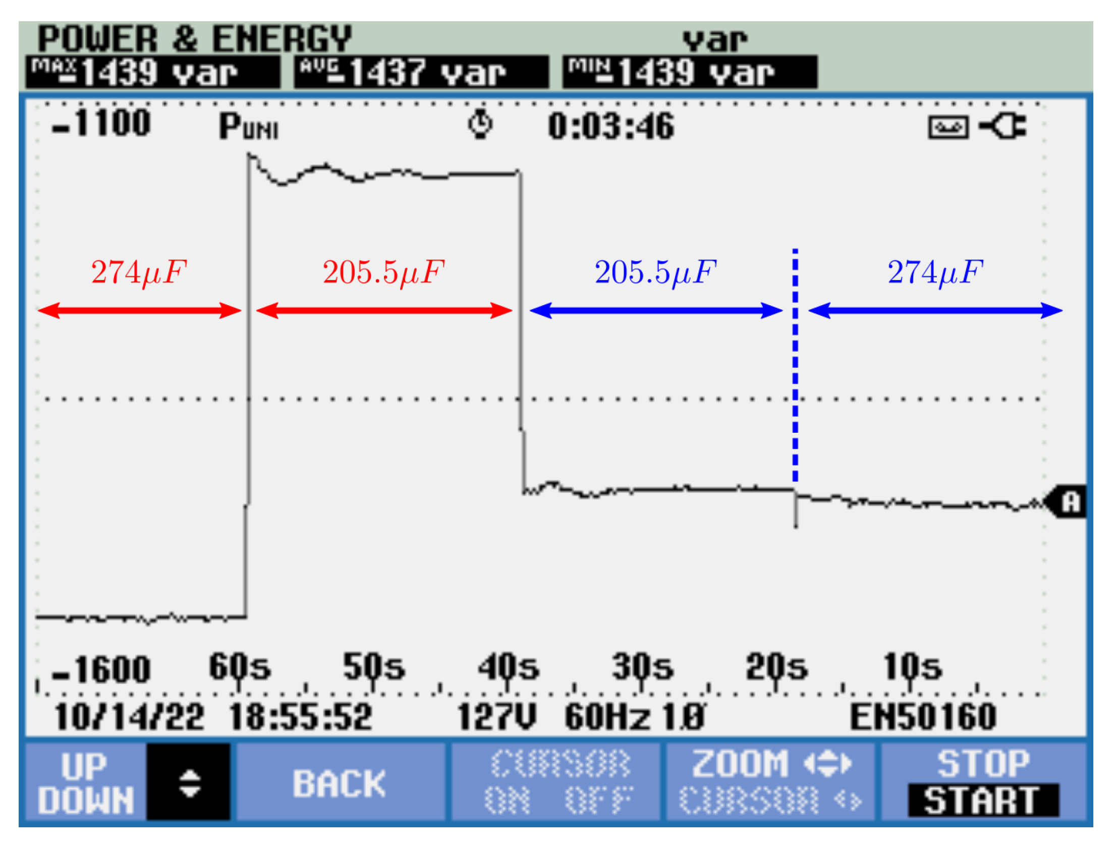
The comparison between the delivered power of the HAPF when operating with and without the estimation algorithm is shown in
Figure 15. In this test, the same 16 A reactive current reference was used. First, the online estimation algorithm was not being used, indicated by the red arrows, and, hence, the delivered power dislocated from its desired value, even for the nominal capacitance value. Once one capacitor was removed, the HAPF delivered power suffered a great change. At the point indicated by 40 s, the online estimation algorithm was activated, indicated by the blue arrows, and the delivered power shifted to the correct value. After a few seconds, the capacitor that was previously removed was once again connected to the capacitor bank, and the delivered power was kept at the reference value. The small variation that occurred at this point was the same as that shown in
Figure 14.
5.2. Dynamic Reactive Power Compensation
When a HAPF is applied to dynamically compensate the reactive power of loads connected to the system, it is important that the power factor at the point of connection is kept unitary. To test how the equipment’s load compensation capability would act under capacitor bank variations, a test load was set, and its power measurement is shown in
Figure 16.
First, the HAPF compensation was tested with the capacitor bank operating with 4 capacitors, with and without the estimation algorithm. The results are shown in
Figure 17. Without the estimation algorithm, a small error was observed at the HAPF point of coupling, as shown in
Figure 17a. This overcompensation indicated that the real value of the capacitor bank capacitance was larger than the one considered by the reference generation algorithm, also indicated by the result shown in
Figure 10. Once the estimation algorithm was activated, the HAPF compensation corrected and a unit power factor was obtained, as depicted in
Figure 17b.
The equipment was then tested with only 3 capacitors connected to the capacitor bank while the same load was being compensated, and the results are shown in
Figure 18. When the estimation algorithm was not active, the HAPF was not capable of fully compensating the load’s reactive power, as depicted in
Figure 18a. This happened because the reference generation algorithm was considering a larger value for the capacitor bank than the one actually connected to the HAPF branch. The result shown in
Figure 18b demonstrates that, when the online estimation algorithm was activated, the HAPF was able to properly compensate the load’s reactive power, and guaranteed a unit power factor at the coupling point.
Finally, regarding the computational burden, the parameters estimation algorithm used four ANFs applied to the system state variables. Each ANF had an execution time of
s (running in a TMS320F28379D at 200 MHz), which resulted in a total time of
s when all four ANFs were being executed. The ANF structure employed was chosen due to its computational efficiency and ease of implementation. As explained in
Section 3, two of the four ANFs were already required by the control reference calculation algorithm, so only two extra ANFs were added, one for
and one for
. The estimation of the system parameters was calculated by Equations (
32) through (
35), which took around
s to be executed, mainly due to the divisions required by the equations. The total execution time for the control algorithm without the parameter estimation was
s (including the PLL and the complete control strategy shown in
Figure 4). After the addition of the proposed parameter estimation algorithm, the total execution time increased to
s, which enabled a sampling frequency of 40,080 Hz.
6. Conclusions
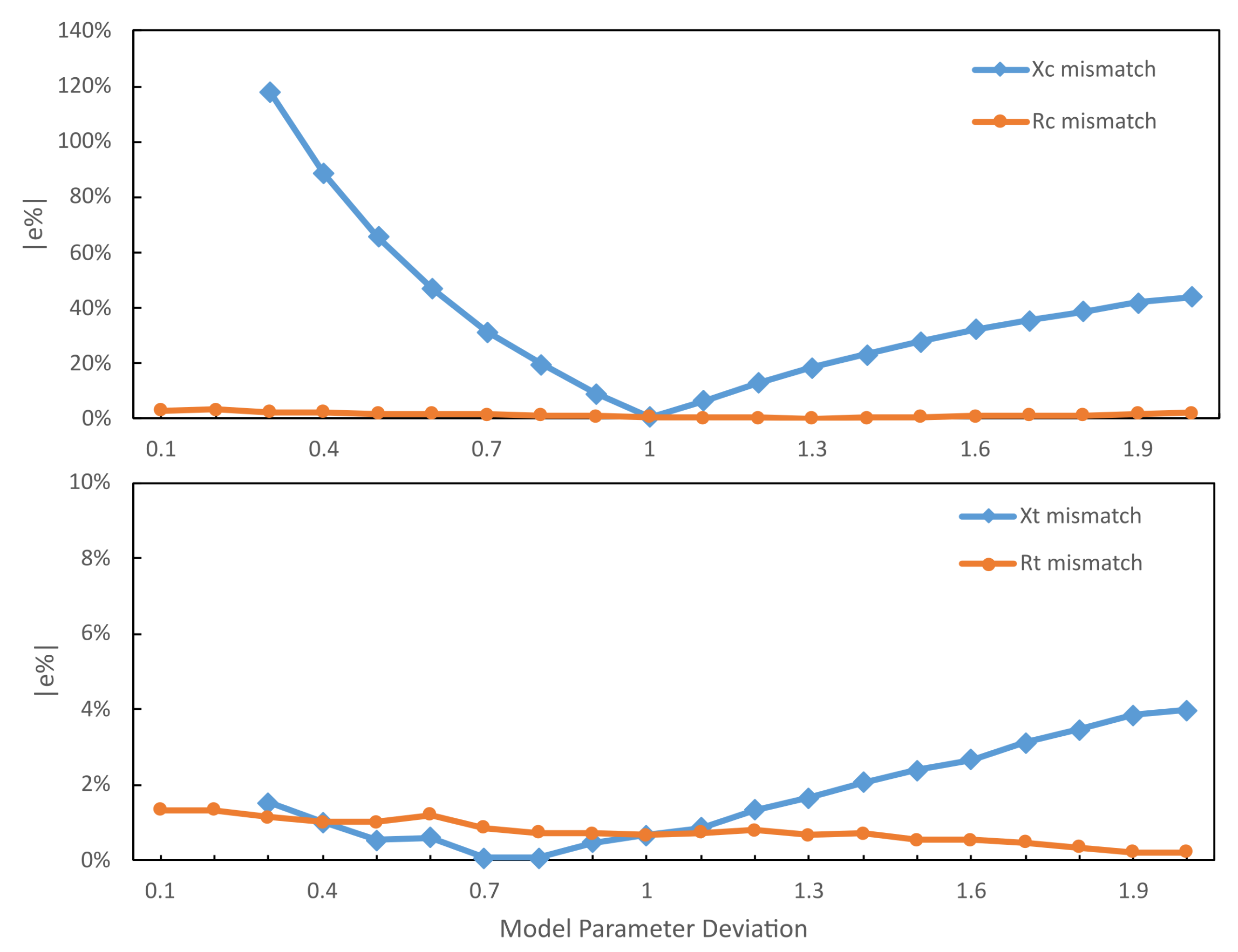
The FCS-MPC is a control technique known to suffer deviations in its response depending on the accuracy of the model parameters. This problem is even more pronounced when the control references are also obtained from the system model. Considering these problems, this work proposed an algorithm to estimate the system parameters used in the control reference calculation during the equipment’s operation. First, a study was conducted to evaluate how each of the parameters’ errors influenced the reference calculation, and it was observed that the most significant deviation was due to uncertainties in the HAPF capacitor bank impedance. Thus, the proposed algorithm was built based on the information provided by four ANFs. Only two extra ANFs were applied, since the other two were already required for the control reference calculations.
The tests performed in the laboratory setup considered, first, a given fixed reactive current reference, and, then, a current reference obtained by the algorithm to compensate load reactive power. In both cases the algorithm showed its capacity to correct the reference deviations caused by model parameter mismatches, improving the current tracking capability and, consequently, the supplied reactive power. Furthermore, since the impedances were being calculated online, the algorithm was also capable of correcting the references when equipment failure occurred, such as the loss of a capacitive cell from the capacitor bank.
The proposed algorithm is capable of estimating the HAPF branch parameters separately. Therefore, it is possible not only to obtain the needed impedances for the adaptation of the control references, but also to keep track of the capacitor bank capacitance. This feature may be used to identify faults in capacitive cells or to actively switch capacitors in and out of the capacitor bank to change the equipment’s operating point, depending on the load reactive power demand, thereby effectively increasing the equipment’s robustness, reliability and operation range for industrial applications.


 ,
, 


