1. Introduction
There are intriguing parallels between the “coal panics” that swept through Britain at the end of the nineteenth century and the “oil panics” that whirl the world today [
1]. Widespread fears exist that reserves of oil will be unable to meet world demand within a decade or so. If long-term stability is to be achieved, significant reforms must clearly be made in our global energy system [
1]. An increasing number of renewable energy technologies are getting relatively mature [
2]; however, the central issue of large scale energy storage remains to be solved. Most of the proposals consider the problem from a technological point of view by investigating new generation of batteries, fuel cells, alternative energy carriers like hydrogen or methanol, etc. There is a general belief in unbroken scientific development, therefore less attention is paid to a possible unfavorable scenario: what happens when no technologically or economically viable new solutions are found in the near future?
Our basic assumption is that existing renewable energy technologies at a sufficient level of penetration can supply most of the demand [
3,
4,
5], however in a very different way than it is provided by the traditional power systems. In the absence of large enough grid storage capacities, energy availability is strongly determined by the instantaneous availability of the resources. It is banal that solar energy is restricted to sunny hours. It is less widely known that the intermittency of wind energy remains surprisingly strong even after integrating over huge geographic areas [
6].
In this work, we compare the electricity demand of a large consumer (a big factory) with a hypothetical supply that is based on wind power exclusively. The measured consumption pattern is composed of characteristic daily, weekly and seasonal cycles following the usual rhythm of human activities. In contrast, wind power availability is determined by the meteorological circumstances and therefore very intermittent. Our analysis is entirely based on high frequency measurements in the factory (power consumption), and at two distant locations of wind turbines (power production) in Hungary. The hypothetical situation is that the factory must switch to electricity provided by wind farms at either one or the other location, furthermore we consider the case when wind electricity is integrated in a common grid.
The main findings are not very different from what one might expect, however they are quantitative. The integration from the two sources is not enough for a continuous supply, even when the wind power capacity is infinitely larger than the average consumption. This is because the area of Hungary is very small, therefore it is quite common that the wind speed nowhere exceeds the cut-in value for some period of time. We demonstrate that scaling up wind power capacities results in a slower than linear improvement in the supply at the cost of an increasing fraction of excess wind electricity. Interestingly, the distribution of length of supply and shortfall intervals exhibits a power-law (scale-free) behavior, and possible consequences are discussed. An important result is that the statistics are practically the same for cyclic and constant average loads, which makes subsequent availability studies much easier.
2. Wind Electricity Resource
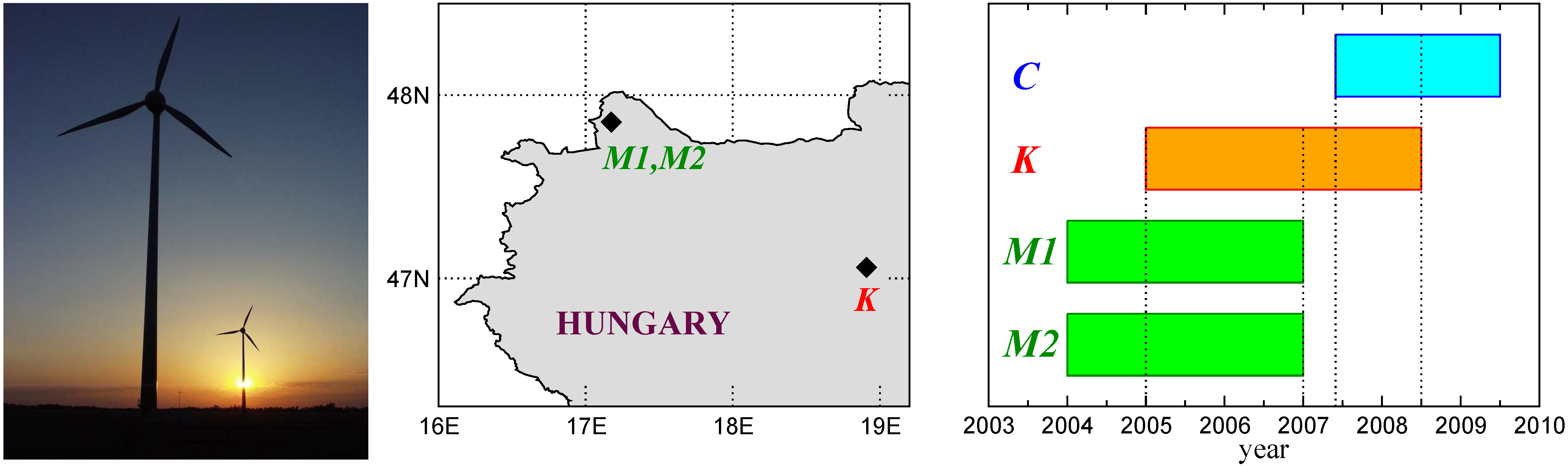
High frequency (10 min) mean wind speed (nacelle anemometer reading at 65 m above ground) and output power data are available to us for three Enercon E-40 (600 kW) wind turbines in Hungary. Two of them (
and
) are located at the geographic coordinates 47.816
N, 17.174
E, near Mosonszolnok (see the photograph in
Figure 1), the third one (
K) is installed at 47.057
N, 18.914
E, in Kulcs. The temporal coverage of the records is illustrated in
Figure 1, right panel, together with the time series for electric power consumption (
C) described in details later. Note that we adopted the standard representation of dates used in Microsoft Excel (day from 1st of January, 1900) in order to facilitate data matching from different sources and lengths.
Figure 1.
Sketch of the geographic setting of the wind turbines and timeline of the records. Heavy diamonds indicate the location of three Enercon E-40 wind turbines
,
(near Mosonszolnok, 47.816
N, 17.174
E) and
K (Kulcs, 47.057
N, 18.914
E). The timeline illustrates the overlapping periods: 06/01/2007–06/30/2008 for
C (consumer) and
K records, and 01/01/2005–12/31/2006 for
K and
M time series. (Photograph: Sándor Zátonyi,
http://www.panoramio.com)
Due to geographic constraints in the Carpathian basin, Hungary is not very rich in wind energy [
7,
8,
9,
10,
11,
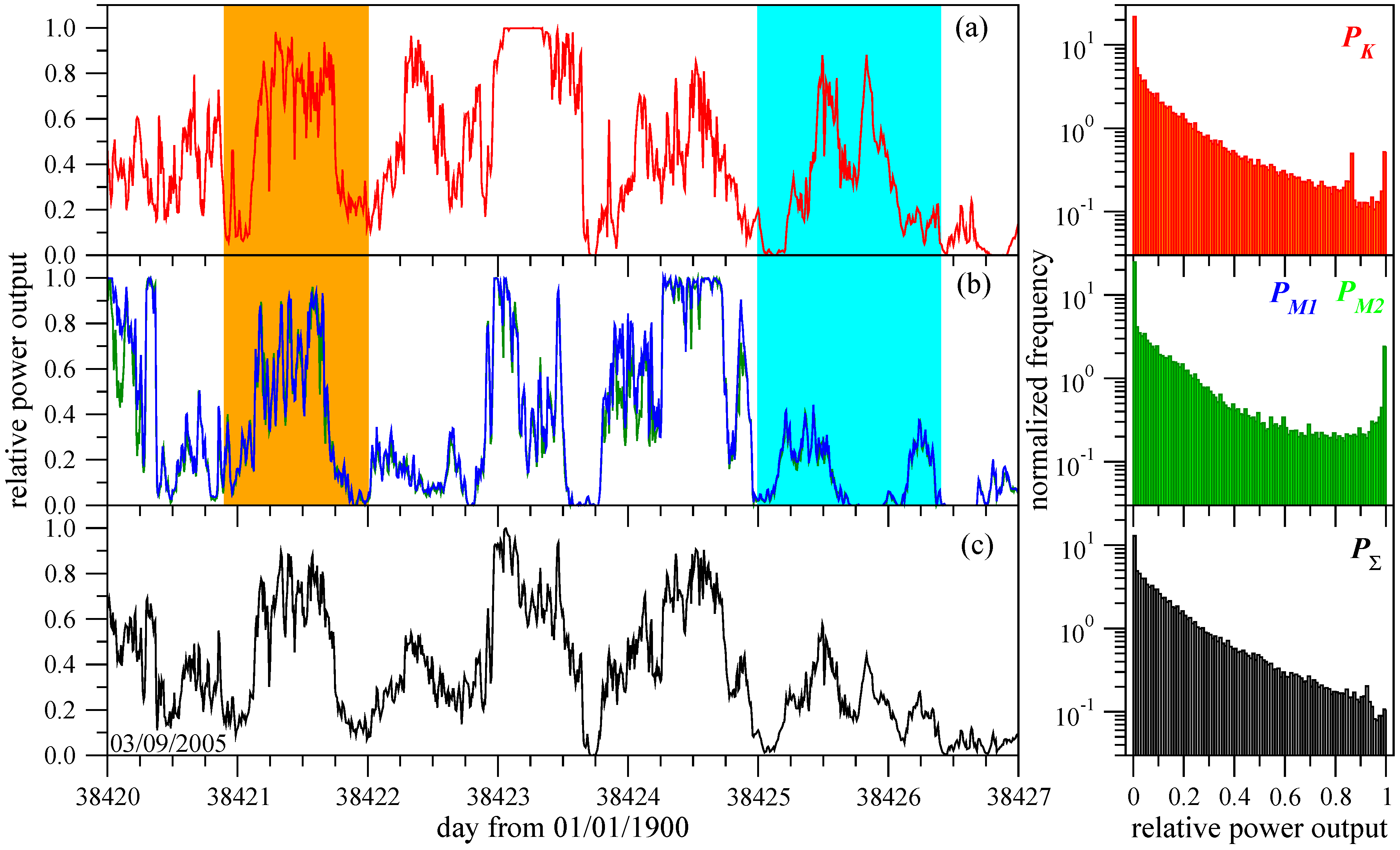
12], and electricity production is extremely intermittent at each site (see
Figure 2). Typical capacity factors (the ratio of mean and rated output power) at working turbines hardly exceed 25%, particular values are at
K: 19.92% ± 23.71%, 17.42% ± 22.61%, 20.89% ± 24.98%; at
: 20.76% ± 11.55%, 22.33% ± 12.58%, 20.27% ± 11.24%; and at
: 21.26% ± 11.66%, 23.16% ± 12.24%, 21.55%±11.58% in three consecutive full years shown in
Figure 1. The proximity of the locations for
and
turbines (their distance is 370 m) yielded almost identical time series (
Figure 2b), significant differences originated from measuring errors, or hardware breakdowns.
As a consequence of the small geographic distance between the
K and
M turbine sites (156 km), one cannot expect the independence of wind speeds. Indeed, the typical correlation length was found around 200–300 km in the study [
6] based on ERA-40 reanalysis data.
Figure 2c clearly illustrates that an integration of 10 min power output in a hypothetical common grid does not result in a drastic improvement considering intermittency. Power integration in the overlapping period of 2005 and 2006 (
Figure 1) is performed by
where we assumed that the two adjacent turbines
and
operate in a “wind farm” mode, thus the two
locations have the same weights. Sporadic missing data (
) were replaced by zeros. Substantially better aggregated output is possible when much larger distances are considered connecting climatologically separated regions [
5,
13].
Figure 2.
Relative power output (instantaneous measured value normalized by the measured peak power of 620 kW) for a period of one week beginning on 03/09/2005. (a) Turbine
K, (b) turbines
(green) and
(blue), and (c) “integrated” power [see Equation (
1)]. Orange (cyan) shading indicates almost synchronous (counter-phase) production. The probability density distributions (normalized frequencies) are shown on the right side, for the
full record lengths indicated in
Figure 1.
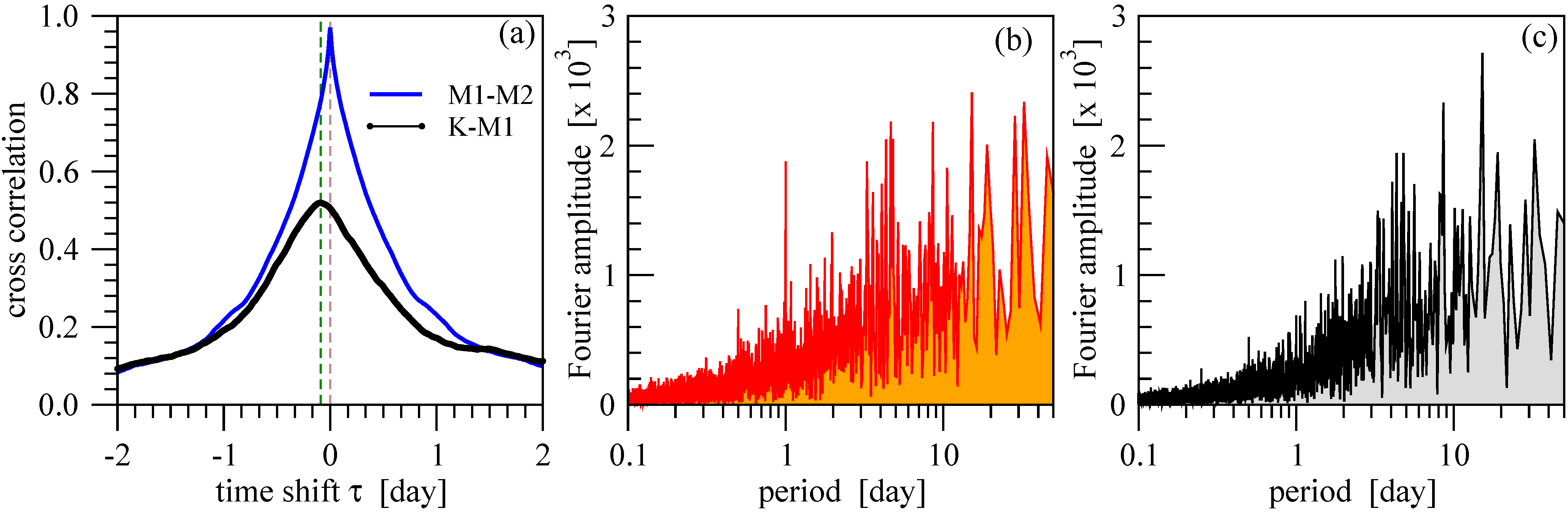
Further relationship between the two turbine sites is revealed by the cross-correlation functions
where
,
τ is the time-shift,
denotes the instantaneous power of average value
and standard deviation
σ, and
indicates temporal averaging. As
Figure 3a clearly shows, the cross-correlation between time series
K and
has a maximum at
day (
hours), the curve is practically the same for
K and
(not shown). This means that the wind speed variations at site
M often determine the changes at site
K occurring a few hours later. Precisely such behavior is expected by checking the maps of the prevailing winds in the territory [
14]. The cross-correlation function for the adjacent turbines (
Figure 3a, blue line) is centered at zero, symmetric, and almost identical with the individual autocorrelation functions given by Equation (
2) with
. This behavior explains why the integrated time series (
Figure 2c) remains almost as intermittent as the original records. The power spectrum provided by standard Fourier analysis for site
K (
Figure 3b) exhibits a weak periodic component around 1 day, which is not present neither at site
M (not shown) nor in the aggregated record (
Figure 3c). This might be connected with the neighboring river basin of Danube at Kulcs.
Figure 3.
(a) Cross-correlation function [see Equation (
2)] for the power records
K and
(black) and
and
(blue). Vertical dashed lines indicate the peak maxima. (b) Normalized Fourier amplitudes for the power record
K. (c) The same for the integrated series shown in
Figure 2c.
Figure 3.
(a) Cross-correlation function [see Equation (
2)] for the power records
K and
(black) and
and
(blue). Vertical dashed lines indicate the peak maxima. (b) Normalized Fourier amplitudes for the power record
K. (c) The same for the integrated series shown in
Figure 2c.
4. Comparison of Supply and Demand
Next we imagine a hypothetical situation where electricity is exclusively provided by wind farms installed at the test sites M and K. It is a highly unrealistic situation since nobody considers wind electricity alone as a working source of baseload supply. Nevertheless, the comparison yields quantitative information on the strength and properties of intermittency.
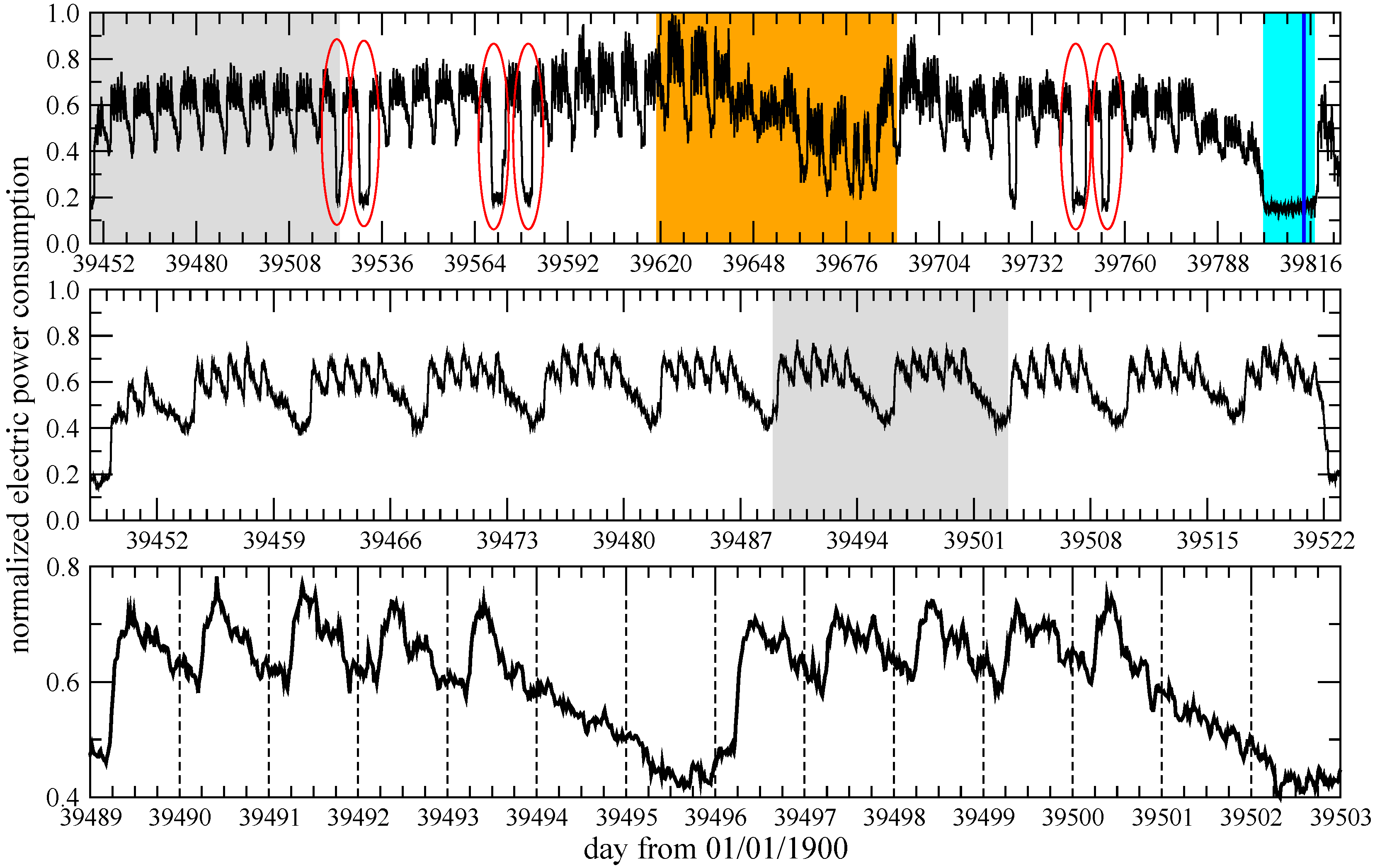
Figure 4.
Relative electric power consumption (instantaneous value normalized by the measured maximum) as a function of time in the year of 2008 (top). Gray shading indicates the period magnified in the middle panel. The orange interval is the main holidays season (from mid-June to end August), light-blue section shows the Christmas-New Year break. The ellipses denote major national holidays (15th of March, Easter, 1st of May, Pentecost, 23th of October, and Hallowmas). The gray shading in the middle panel denotes the two weeks magnified at the bottom.
A key parameter of the analysis is the total wind power capacity
. It is meaningless to “install” less capacity than it is required by the consumer in a full year. As we listed in
Section 2., typical capacity factors are around
for turbines in Hungary, thus the installed rated power
must exceed either the peak or average consumption (
or
) by a factor of 5. A coefficient
F characterizes the excess capacity through
such that
purports
.
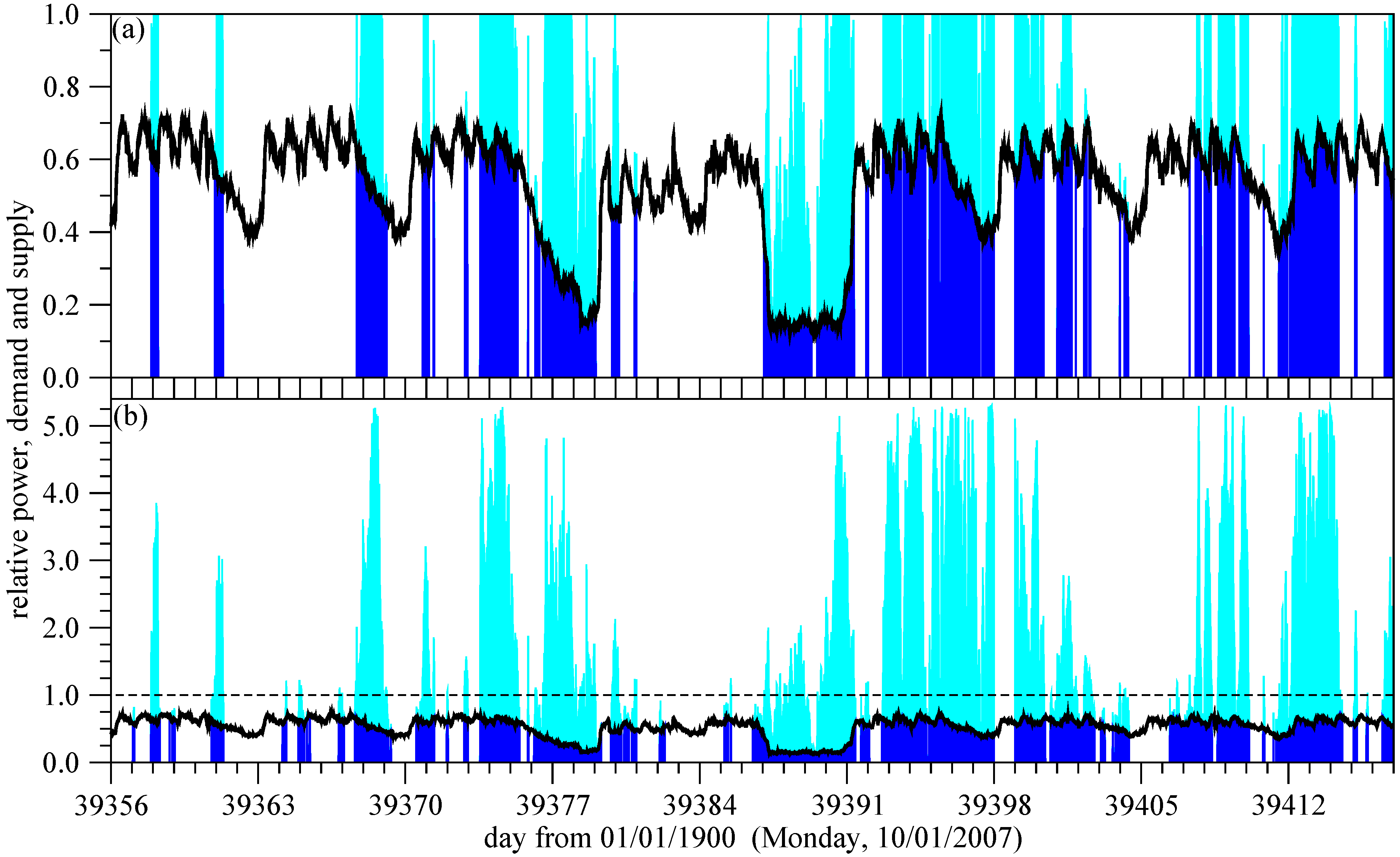
Figure 6 illustrates how supply and demand fit in two windy months in 2007 for two values of factor
F. Besides the intermittency, two aspects are remarkable. Firstly, when adequate supply is given by wind power, it is almost always in conjunction with considerable excess electricity production. Secondly, when the total rated power is increased by a factor of 2 (in the case of our consumer this means investing in many dozens of new turbines), the supply does not improve drastically; a number of white intervals remain which indicates electricity shortfall.
In order to characterize the improvement of supply by increasing the total rated capacity
, we repeated the comparison for years 2005 and 2006 with the individual and aggregated wind power records and the consumption pattern formed by gluing the average weekly cycle (
Figure 5a) as a function of
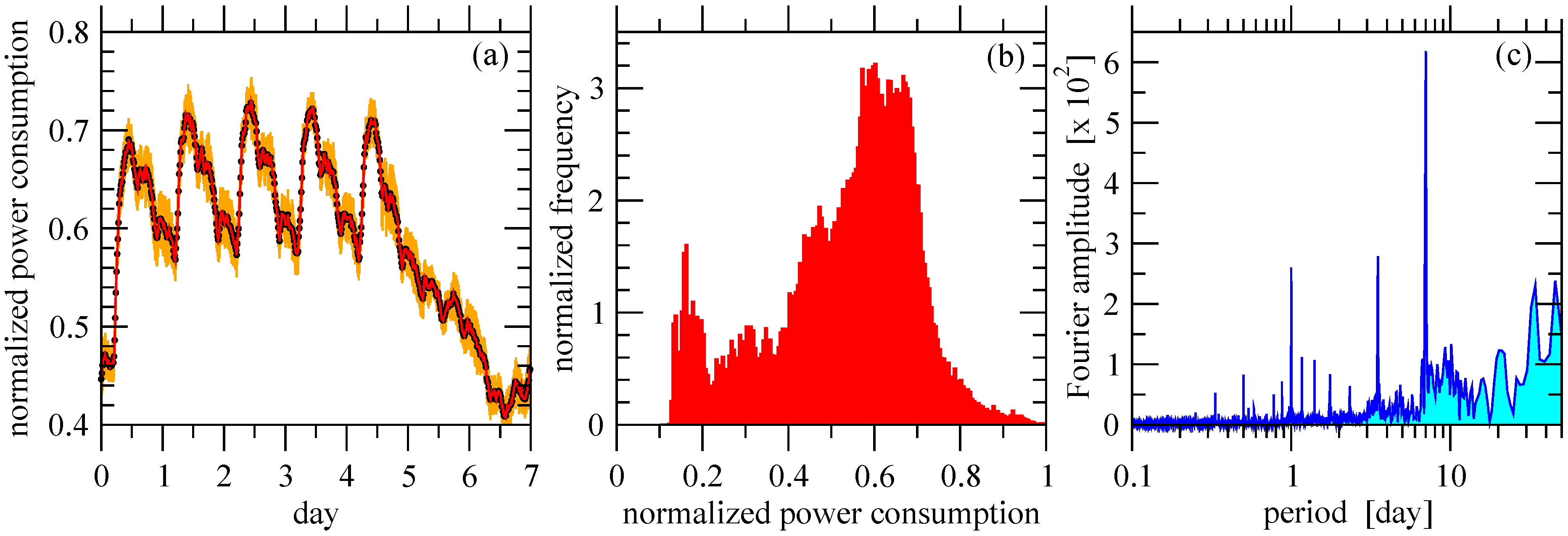
Figure 5.
(a) Weekly power consumption pattern (black) extracted by averaging 9 regular working weeks in 2008 starting from day 39454 (
Figure 4, middle). Red line shows the same curve with a temporal resolution of 10 min, orange is the standard deviation. (b) Histogram of the power consumption obtained from the
full record. (c) Fourier analysis reveals the strong daily and weekly cycles, the other thin peaks are harmonics.
Figure 6.
Matching of wind power supply (blue shading) with demand (black curve) in two full months (October–November, 2007) for wind power record
, see
Figure 2a]. Light blue shading indicates excess wind power. (a)
, (b)
[see Equation (
3)]. The vertical scale is extended to illustrate excess production.
factor
F. The result is shown in
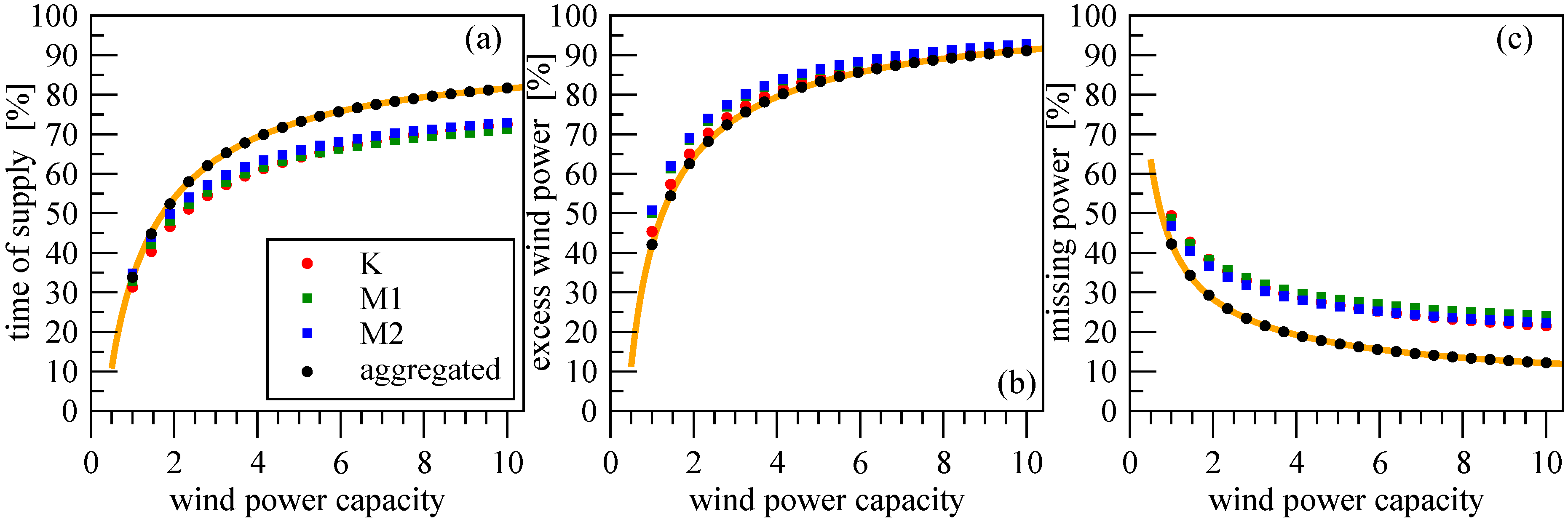
Figure 7a. The benefit of wind power aggregation from distant sites is clear, still the curve exhibits quick saturation for this case as well. The functional form for the total time of supply
:
provides a good quality fit for each curve. We show only one for the aggregated wind power (
Figure 7a, orange line) with fitted values
%,
,
, and
. The asymptotic value
% is a consequence of lull periods when the wind speeds remain below cut-in value at both sites. Note that the supply level of 1/2 (
%) requires around
, which means 10 times larger installed capacity (with
) than the mean consumption.
Figure 7.
(a) Total time of supply
as a function of installed wind power capacity [expressed through factor
F in Equation (
3)] for the individual and aggregated wind power records, see legends. 104 weeks with the pattern in
Figure 7a are considered in the comparison. The orange line illustrates the fit by Equation (
4). (b) Excess wind power
E as a function of
F. The orange line is a fit by Equation (
4) (
T is replaced by
E). (c) Missing power
in periods where wind energy production is nonzero, but remains below the demand. The orange line is a fit by Equation (
5).
It is clear that a growing total rated capacity results in an increasing fraction of excess wind power
E not required by the very consumer (see
Figure 6b).
Figure 7b illustrates this fraction as a function of factor
F, the behavior is also stretched exponential according to Equation (
4). The essential difference is that the asymptotic value (belonging to the limit
) converges to the maximum
% for each curve, the other parameters for the aggregated wind power record are
,
, and
. This can be understood, because the consumption is finite, but nothing limits (mathematically) the installed capacity
.
Finally, we evaluated the decreasing portion of periods when nonzero wind power—less than the demand—is produced. In such situations the missing power
must be complemented from other sources. Limiting cases are the full supply periods with
, and the opposite case when arbitrarily small wind power production is scaled up by
F to fulfill the instantaneous requirement, thus
is the total demand when the wind power is exactly zero. The orange line in
Figure 7c indicates again a stretched exponential relaxation
with parameter values
%,
,
, and
. We emphasize that the functional forms Equations (
4) and (
5) serve only to estimate results out of the tested range of
F, and a theoretical explanation is not intended.
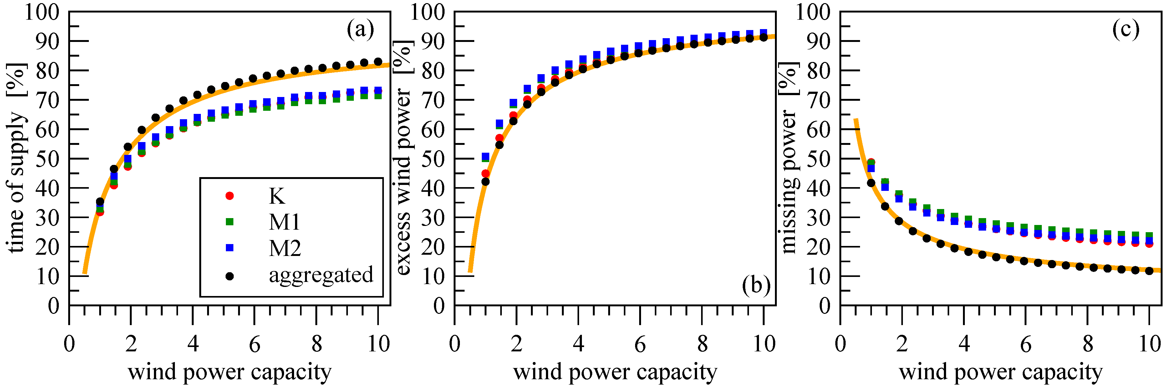
Figure 8.
The same as
Figure 7, by assuming a
constant relative power consumption of 0.59. Note that the orange lines are
not fitted here, there are identical with the ones in
Figure 7.
Figure 8.
The same as
Figure 7, by assuming a
constant relative power consumption of 0.59. Note that the orange lines are
not fitted here, there are identical with the ones in
Figure 7.
Figure 8 exhibits curves almost identical to
Figure 7, however we think that this is an important result. Here the consumption pattern is simply replaced by the constant average value, nevertheless the results remain very close to the above ones. To illustrate this fact, we show exactly the same fits obtained in
Figure 7 (
Figure 8, orange lines), the symbols belong to the repeated evaluation assuming constant consumption.
Figure 6b demonstrates that the fluctuations of power consumption are are much smaller than the production, therefore the former can be replaced by a constant value, indeed. Further studies can benefit a lot from this observation, because it seems that power consumption data with high resolution are not imperative to characterize intermittency of electricity production, when data of the resource are available.
The intermittent behavior of wind energy production is related to turbulence in the wind field. It is known for decades that the so called “level-crossing” statistics, i.e., the length distribution of time intervals above or below a given threshold value, has a power-law shape for horizontal wind speeds [
15,
16]. In our analysis, a closely related statistics is the length distribution of continuous time intervals of adequate supply
or electricity shortfall
. Level-crossing statistics of wind speeds is certainly in the background, however wind electricity generation represents a nonlinear filter by the power-curve of turbines [
6,
13], and the “level” to cross (power demand) is changing in time. Nevertheless we found that the empirical frequency distributions for both continuous intervals
and
obey power law, examples for two series (
and
) presented in
Figure 9 and
Figure 10. We emphasize that we extracted the frequency distributions for records
and
as well, and they have the same shape.
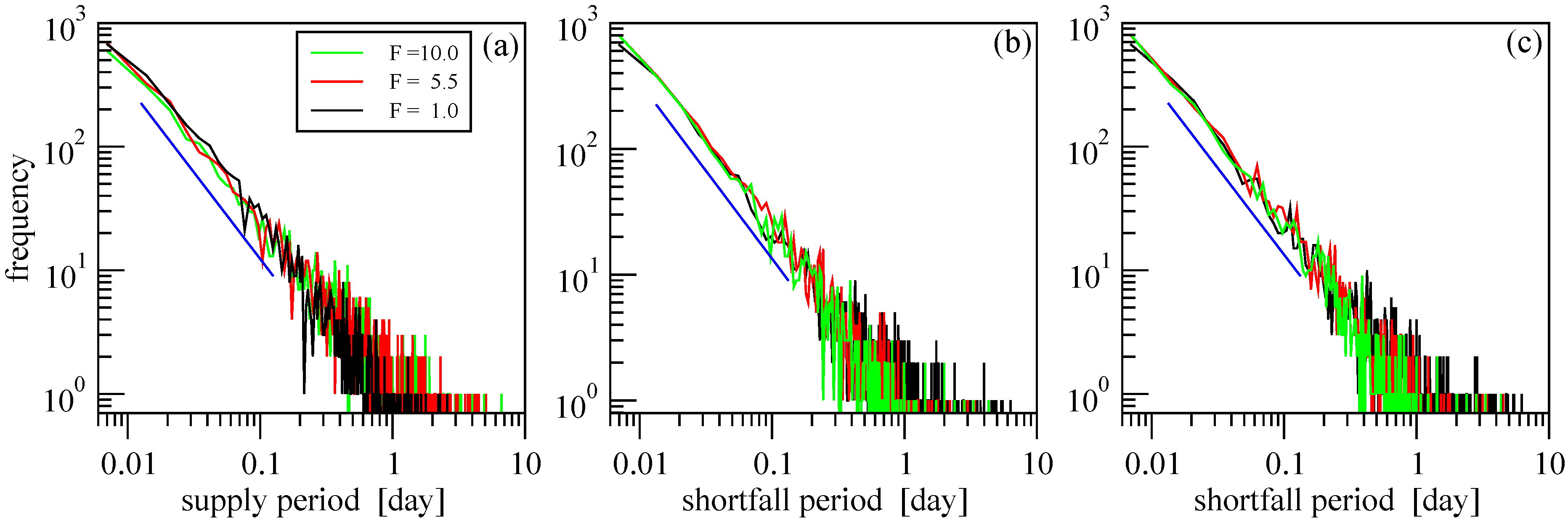
Figure 9.
Length distribution of continuous periods of (a) supply, (b) shortfall, and (c) shortfall with constant consumption at three values of F (see legends) for wind power record . (Note the double logarithmic scale.) Blue lines indicate a power-law with exponent value .
Figure 9.
Length distribution of continuous periods of (a) supply, (b) shortfall, and (c) shortfall with constant consumption at three values of F (see legends) for wind power record . (Note the double logarithmic scale.) Blue lines indicate a power-law with exponent value .
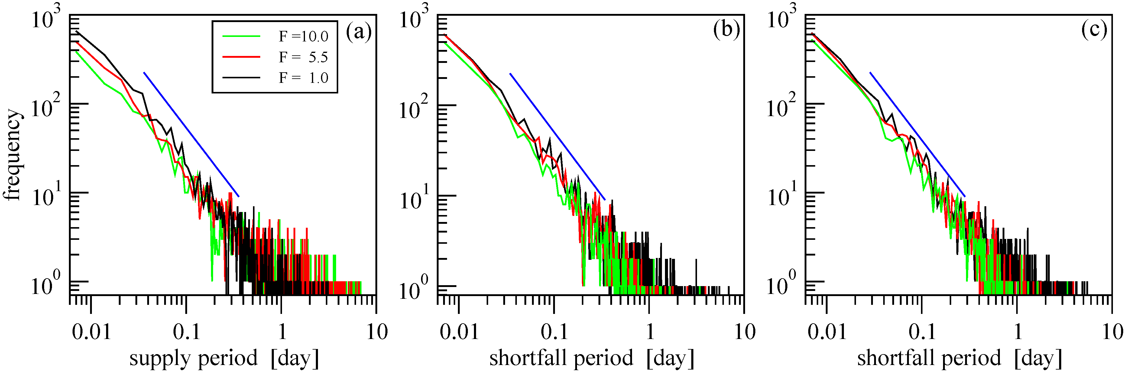
Figure 10.
The same as
Figure 9, for the aggregated wind power record
.
Figure 10.
The same as
Figure 9, for the aggregated wind power record
.
Table 1.
Maximum period lengths (in days) for continuous supply (
) and shortage (
) at three different total power factor
F. Wind power records
and the aggregated one
[see Equation (
1)] are evaluated in years 2005–2006.
Table 1.
Maximum period lengths (in days) for continuous supply () and shortage () at three different total power factor F. Wind power records and the aggregated one [see Equation (1)] are evaluated in years 2005–2006.
| F | | | | |
|---|
| 1.0 | 2.62 | 3.18 | 6.48 | 7.02 |
| 5.5 | 5.08 | 6.64 | 4.38 | 4.11 |
| 10.0 | 6.64 | 6.86 | 4.38 | 3.50 |
A closer look of the curves reveals that a simple power law cannot fit all the data, and systematic deviations are characteristic mostly at the tails. The decay gets slower for periods of supply when the total installed capacity
is increased, while the opposite is true for periods of shortfall. The exponent values are difficult to obtain because of the apparent noise, instead we show the absolute maxima in 2005–2006 (
Table 1) which indicate the same tendency. A saturation effect is also obvious here, as no further increase of
can elongate supply periods when all the intervals of shortage have exactly zero wind power production.
5. Conclusions
It is almost trivial that at a single location, it is not possible to guarantee power from wind turbines at any time. With the large-scale deployment of intermittent resources today, backup generators that can be quickly connected to the grid are needed, which increases the cost of investment and maintenance. When different intermittent energy sources are combined with each other or over large geographical regions, they are much less intermittent than at one location [
13,
17]. Nevertheless a quantitative characterization of different sources is a difficult task, the design of an optimal “energy portfolio” is far from being solved [
17,
18].
Here we presented a case study on supply and demand relationship based on measured data in Hungary. We have found that the aggregated output from two wind farms, designed to produce the same amount of electric power as the annual demand, can provide adequate supply for 34% in a year. The rest of the output arises due to the unused excess electricity. Two times larger total installed capacity increases this interval to be 52%, however any further increase has far less efficiency due to a stretched exponential saturation to the limiting value of 87%.
Although the consumption pattern is composed of regular daily and weekly cycles (interrupted by shorter or longer periods of low activity), the length distribution of supply and shortfall periods has a scale-free, power-law decay, even when the time integrated wind energy production is ten times larger than the annual consumption. It is obvious, that supply intervals shorter than a few hours cannot be exploited economically, therefore wind (in Hungary) can never provide the baseload power, irrespective of the total installed capacity.
Further studies on the availability of renewable energy sources are strongly promoted by the finding that the periodic consumption pattern is statistically very close to the case of steady demand. This is again the consequence of strong intermittency: wind energy is produced by huge fluctuations between exactly zero and five times of the mean value.


