1. Introduction
The lithium-ion battery (LIB) is popular in consumer electronics. Beyond consumer electronics, the LIB is also growing in popularity for automotive applications such as hybrid electric vehicles and battery electric vehicles and stationary energy storage systems for renewable energy produced by sunlight and wind. Lithium iron phosphate (LiFePO
4 or LFP), which was reported by Padhi
et al. [
1] in 1997, is one of the most promising cathode materials for a LIB owing to its low cost, non-toxicity, and high abundance of iron. Despite the numerous advantages of LFP, its low electronic and ionic conductivities seriously limit its rate capability [
2,
3,
4]. To overcome these limitations, many studies have been carried out, including particle size reduction [
5,
6,
7], coating [
8,
9,
10], and doping [
11,
12,
13]. Even though the proper fabrication process of LFP has been identified, the composition of a LFP cathode consisting of active material, conductive additives, and binders should be optimized in order to tailor the LFP battery to a specific application.
Mathematical modeling serves an important role when optimizing the composition of battery electrodes because almost limitless design iterations may be performed by using simulations [
14]. There have been many previous studies on modeling LIBs, and reviews of LIB models are available in references [
15,
16,
17]. Doyle
et al. [
18] developed a one-dimensional model for a LIB derived from a porous electrode and concentrated solution theory. Others [
19,
20,
21,
22] used or modified the model of Doyle
et al. [
18]. Kwon
et al. [
23] presented a different approach from the rigorous porous electrode model [
6,
7,
8,
9,
10] to predict the discharge behavior of a LIB cell. They developed a model to calculate the potential and current density distribution on the electrodes of a LIB cell on the basis of charge conservation. Even though they do not include lithium ion transport and the potential distribution in the electrolyte phase in their model, the modeling results are in good agreement with the experimental measurements. By not calculating the distributions of the lithium ion concentration and electrolyte-phase potential, the model of Kwon
et al. [
23] significantly saves computation time as compared to the rigorous porous electrode model, while maintaining the validity of the model, even at high discharge rates. Kim
et al. [
24,
25,
26] performed two-dimensional thermal modeling to predict the thermal behavior of a LIB cell during discharge and charge on the basis of the potential and current density distributions obtained by the same procedure used by Kwon
et al. [
23]. They reported good agreement between the modeling results and the experimental data. Kim
et al. [
27] extended their thermal model [
24,
25,
26] to accommodate the dependence of the discharge behavior on the environmental temperature.
In this work, a one-dimensional model obtained by reducing the spatial dimension of the two-dimensional model of Kim
et al. [
24,
25,
26] owing to the cylindrical symmetry of a coin cell is presented to investigate the effects of the cathode composition on the discharge behavior of a LFP battery cell comprising a LFP cathode, a lithium metal anode, and an organic electrolyte. Validation of the modeling approach is provided via a comparison of the modeling results with experimental measurements.
2. Mathematical Model
A coin-type LFP battery cell comprising a LFP cathode, a lithium metal anode, and an organic electrolyte is modeled in this work.
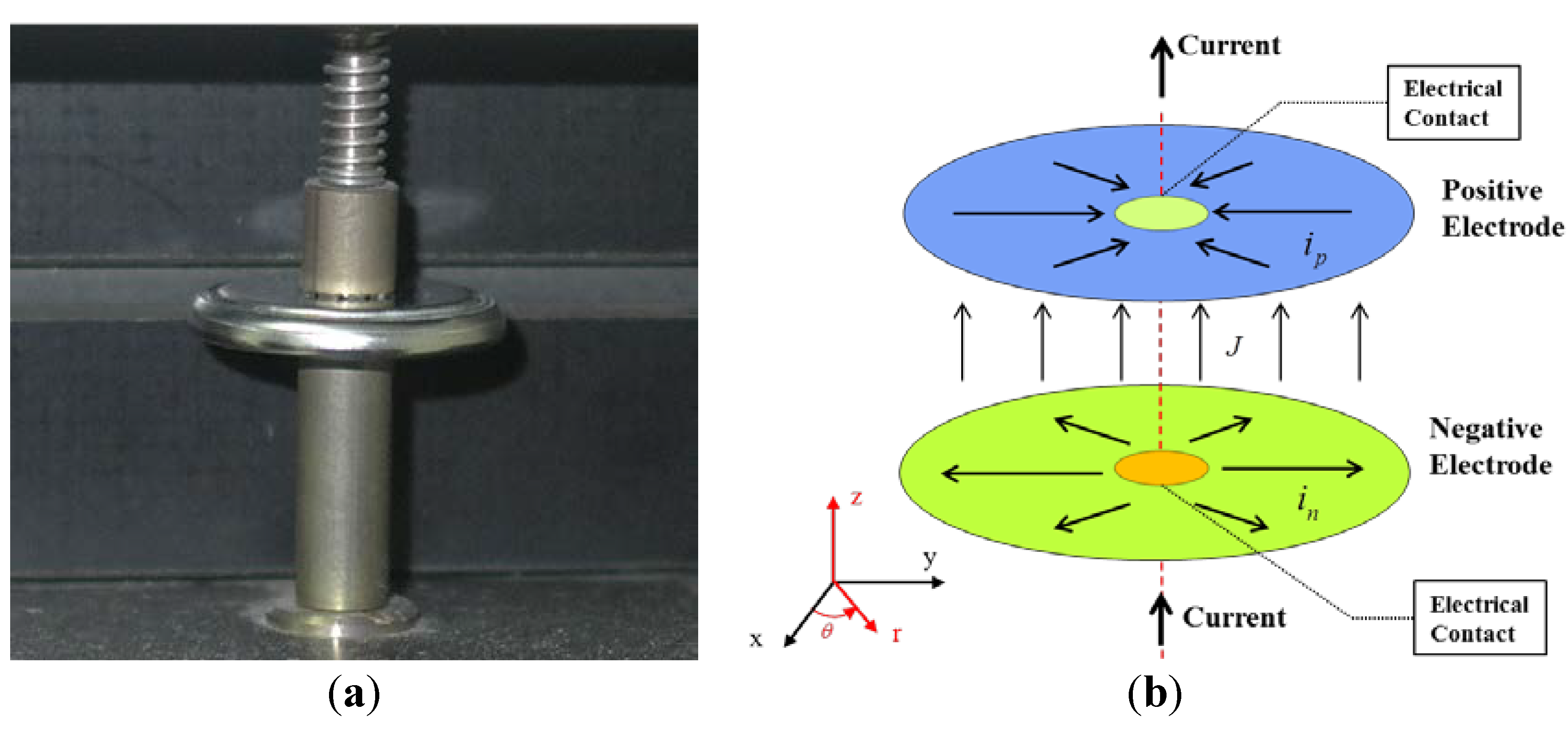
Figure 1a shows a photograph of the coin cell mounted on a jig. The electrical components of the jig are plated with gold to create good electrical contact between the electrical lead from the battery cycler and the battery sample. A schematic diagram of the two-dimensional currents in the two parallel circular electrodes during discharge is shown in
Figure 1b. The distance between the electrodes is assumed to be so small that the current between the electrodes would be perpendicular to them. The two-dimensional currents on the positive and negative electrodes in
Figure 1b are assumed to have circular symmetry with respect to the axis passing through the centers of the circular electrodes. Then, the two-dimensional currents on the electrodes may be reduced to one-dimensional currents in terms of the radial coordinate,
r, in
Figure 1b.
Figure 1.
(a) Photograph of the coin cell mounted on the jig; and (b) schematic diagram of the currents in the two parallel circular electrodes during discharge.
Figure 1.
(a) Photograph of the coin cell mounted on the jig; and (b) schematic diagram of the currents in the two parallel circular electrodes during discharge.
The modeling procedure used to calculate the potential and current density distribution on the electrodes is similar to that of the two-dimensional model of Kwon
et al. [
23]. From the continuity of the current on the electrodes, the following equations are derived:
where
ip,r and
in,r are the
r components of the linear current density vectors [current per unit length (A·m
−1)] in the positive and negative electrodes, respectively; and
J is the current density [current per unit area (A·m
−2)] transferred through the separator from the negative electrode to the positive electrode.
Rc and
R denote the radii of the electrical contact and the coin cell, respectively. According to Ohm’s law,
ip,r and
in,r are expressed as follows:
where
rp and
rn are the resistances (Ω) of the positive and negative electrodes, respectively;
Vp and
Vn are the potentials (V) of the positive and negative electrodes, respectively;
rp and
rn are calculated as described in references [
23,
24,
25]. The following Poisson equations for
Vp and
Vn are obtained by substituting Equations (3) and (4) into Equations (1) and (2), respectively:
The relevant boundary conditions for
Vp are:
The first boundary condition in Equation (7) means that the linear current density through the electrical contact of length
(cm) has a value of
.
I0 is the total current (A) through the electrical contact in the constant-current discharge mode, which is a function of time. The second boundary condition in Equation (8) implies that there is no current through the electrode edge. The boundary conditions for
Vn are:
The first boundary condition in Equation (9) means that the potential at the electrical contact of the negative electrode has a fixed value of zero as the reference potential. The second boundary condition in Equation (10) implies the same as in the case of Vp.
The current density,
J, of Equations (1) and (2) is a function of the potentials of the positive and negative electrodes. The functional relationship between the current density and the electrode potentials depends on the polarization characteristics of the electrodes. In this study, the following polarization expression used by Tiedemann and Newman [
28] and Newman and Tiedemann [
29] is employed:
where
Y and
U are the fitting parameters. The physical meaning of
U is similar to the equilibrium potential of the battery cell, and
Y may be regarded as a reaction rate constant of an electrochemical reaction as discussed in reference [
27]. As suggested by Gu [
30],
U and
Y are expressed as functions of the depth of discharge (
DOD) as follows:
where
a0–
a11 are the fitting parameters. The details of the procedures to obtain
a0–
a11 are given in reference [
27]. The fitting parameters used to calculate the potential distributions on the electrodes are listed in
Table 1. The meaning of cases A–B in
Table 1 is given in the following Experimental Section.
Table 1.
Fitting parameters used to calculate the potential distributions on the electrodes.
Table 1.
Fitting parameters used to calculate the potential distributions on the electrodes.
| Parameter | Case A | Case B | Case C |
|---|
| a0 (V) | 3.57 | 3.51 | 3.61 |
| a1 (V) | −7.31 | −3.24 | −6.81 |
| a2 (V) | 58.47 | 23.97 | 52.13 |
| a3 (V) | −169.47 | −67.31 | −148.56 |
| a4 (V) | 202.64 | 78.68 | 175.68 |
| a5 (V) | −85.12 | −32.38 | −73.08 |
| a6 (S m−2) | 362.95 | 269.72 | 236.88 |
| a7 (S m−2) | −228.76 | −163.33 | 3.62 |
| a8 (S m−2) | 298.66 | 425.62 | −509.07 |
| a9 (S m−2) | −2554.81 | −989.2 | 3.13 |
| a10 (S m−2) | 4129.45 | 318.89 | 729.42 |
| a11 (S m−2) | −2000.35 | 159.13 | −440.37 |
3. Experimental Section
To obtain LFP, a solid state reaction using ball milling was performed for 3 h at a rotational speed of 250 rpm with stoichiometric amounts of lithium carbonate (Li
2CO
3, Sigma-Aldrich, St. Louis, MO, USA), iron(II) oxalate (FeC
2O
4·2H
2O, Sigma-Aldrich), ammonium di-hydrogenophosphate (NH
4H
2PO
4, Sigma-Aldrich), and 3% carbon black as a carbon source precursor. The resulting mixture was dried at 50 °C for 16 h in a drying oven and then heated in a tube furnace at 600 °C in an atmosphere with a gas mixture of 95% Ar and 5% H
2 for 10 h. The carbon-coated LFP was mixed with polyvinylidene fluoride (PVDF) as binder and acetylene black (
w/
w) as conductive additive in N-methylpyrrolidone (NMP) solvent and coated onto an Al foil. After drying in a vacuum oven at 80 °C for 12 h, the electrode thickness was measured to be 60 μm, and the mass of active material was about 5–7 mg·cm
−2. The cathode was placed in a standard coin cell (2032 type) with 1 M LiPF
6 in an ethylene carbonate/dimethyl carbonate/ethylmethyl carbonate (EC/DMC/EMC) solution as an electrolyte and a lithium foil as a counter electrode. A Maccor 4000 battery cycler (Maccor, Tulsa, OK, USA) with a cut-off voltage of 2.5 V was used to carry out galvanostatic discharging of the LFP battery cell at discharge rates of 0.1C, 0.5C, 1.0C, and 2.0C for three different compositions of the LFP cathode. The three different compositions of the LFP cathode are referred to as cases A–C and are listed in
Table 2.
Table 2.
Compositions of the lithium iron phosphate (LFP) cathode for cases A–C.
Table 2.
Compositions of the lithium iron phosphate (LFP) cathode for cases A–C.
| Case | Composition of the cathode (wt%) |
|---|
| Active material | Conductive additive | Binder |
|---|
| Case A | 85 | 10 | 5 |
| Case B | 87.5 | 7.5 | 5 |
| Case C | 90 | 5 | 5 |
4. Results and Discussion
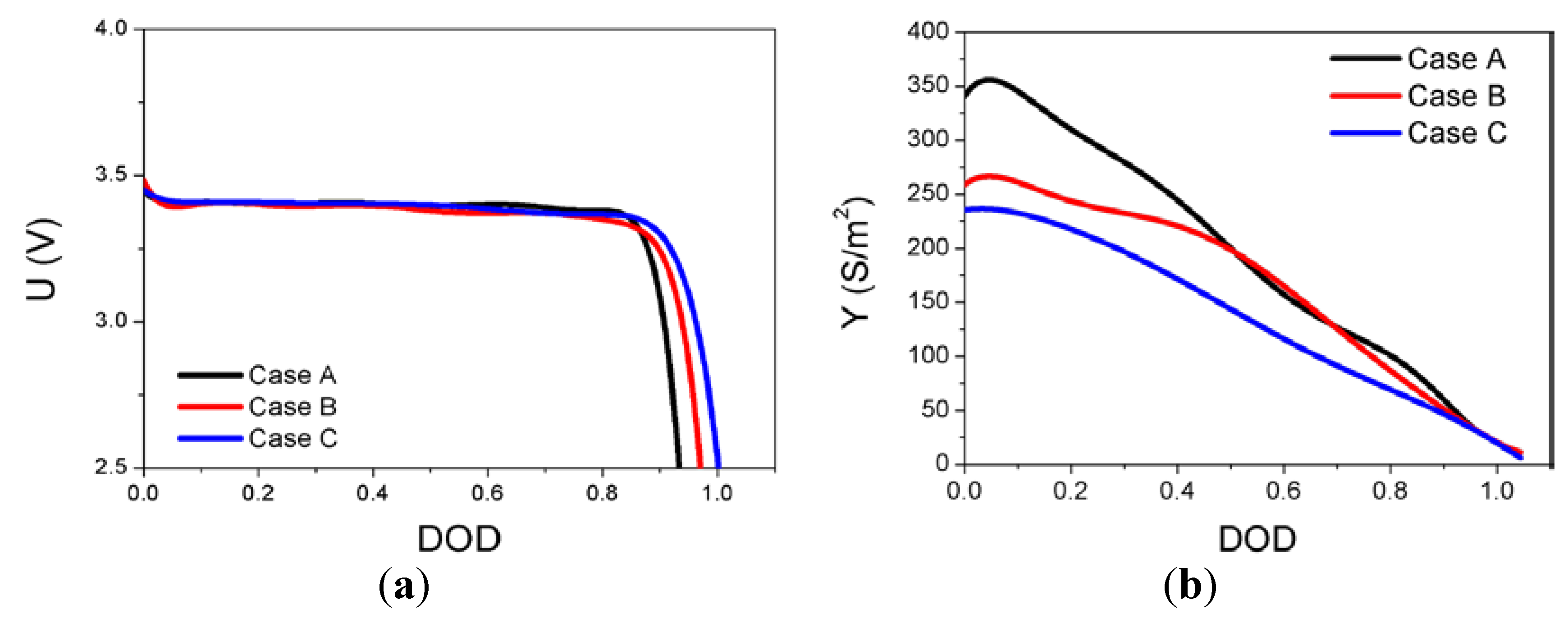
The solutions to Equations (5) and (6) subject to the associated boundary conditions are obtained by using a finite element method. For three different compositions of the LFP cathode,
U and
Y are obtained as functions of
DOD, as expressed in Equations (12) and (13), to provide the best fit of the modeling results to the experimental data and are plotted in
Figure 2.
Figure 2.
(a) U as a function of depth of discharge (DOD); and (b) Y as a function of DOD.
Figure 2.
(a) U as a function of depth of discharge (DOD); and (b) Y as a function of DOD.
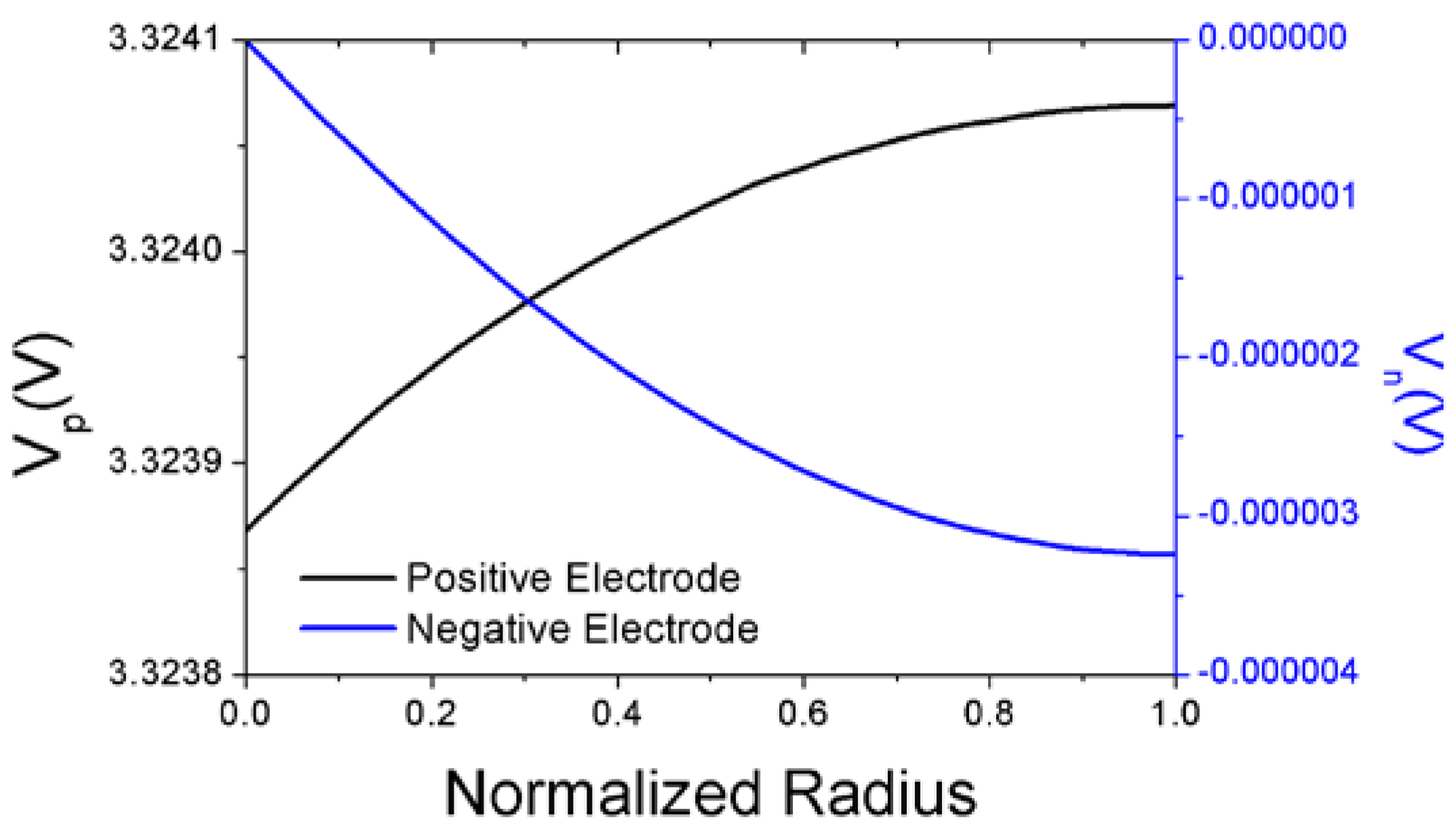
In
Figure 3, the potential distributions of the positive and negative electrodes are plotted when the battery cell of case A is discharged with the discharge rate of 2.0C at the
DOD value of 0.2 as a demonstration of the potential distributions obtained from the solutions of Equations (5) and (6). The potential of the positive electrode near the outer edge of coin-type cell has a higher value as compared to that near the electrical contact at the center of coin-type cell. This conforms to the expectation that the current flows from the outer edge of the coin-type cell to the center of the cell in the positive electrode during discharge as shown schematically in
Figure 1b. The potential of the negative electrode near the center of coin-type cell has a higher value as compared to that near the outer edge of coin-type cell. This seems rational, because the direction of current flow is from the center of the cell to the outer edge of the cell during discharge as shown in
Figure 1b. The battery cell potential calculated from modeling is the difference between the values of
Vp and
Vn shown in
Figure 3 when the normalized radius defined as (
r−Rc)/(
R−Rc) is zero.
Figure 3.
Potential distributions of the positive and negative electrodes as a function of normalized radius.
Figure 3.
Potential distributions of the positive and negative electrodes as a function of normalized radius.
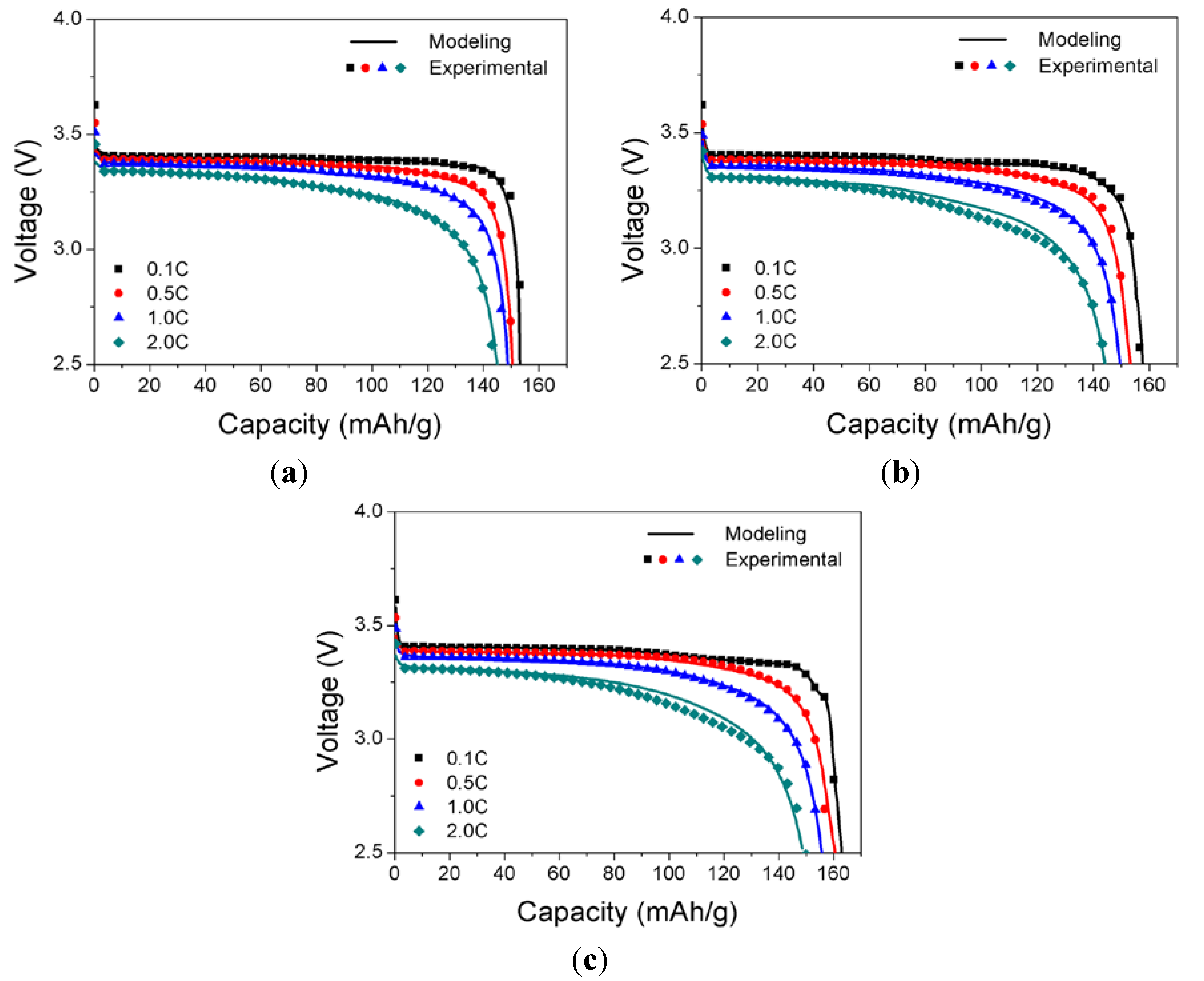
To test the validity of the modeling approach, the cell voltage of the LFP battery calculated from the modeling as described in the above has to be compared with the experimental measurements obtained with various discharge rates for the different compositions of the LFP cathode. With the object of the model validation, the calculated discharge curves from the model using
U and
Y presented in
Figure 2 are compared with the experimental data with discharge rates ranging from 0.1C to 2.0C for three different compositions of the LFP cathode in
Figure 4. The experimental discharge curves are generally in good agreement with the modeling results based on the finite element method, although there is some deviation between the experimental and modeling discharge curves for cases B and C at high C rates. The modeling approach presented in this work is simply changing the key modeling parameters
U and
Y as the functions of
DOD for different compositions of cathode. This approach enabled the model to capture all of the salient features of the discharge characteristics of the cell voltage, such as the initial rapid drop and subsequent plateau followed by a continuous decrease to the cutoff voltage of 2.5 V at various discharge rates from 0.1C to 2.0C for the three different compositions of the LFP cathode. This demonstrates the validity of the modeling approach for predicting the effects of the cathode composition on the discharge behavior of a LFP battery cell comprising a LFP cathode, a lithium metal anode, and an organic electrolyte.
Figure 4.
Comparison between the experimental and modeling discharge curves with discharge rates ranging from 0.5C to 5C: (a) case A; (b) case B; and (c) case C.
Figure 4.
Comparison between the experimental and modeling discharge curves with discharge rates ranging from 0.5C to 5C: (a) case A; (b) case B; and (c) case C.
In order to estimate the discharge behavior of a LFP battery cell for a broader range of cathode compositions other than the three compositions in
Figure 4 for which the experiments are performed,
U and
Y are calculated as functions of
DOD and the cathode composition by using the Kriging method. The Kriging method is widely used in the geostatistical science and the software library is open to the public [
31]. The Kriging method provides an optimal interpolation or extrapolation for the unknown values of the function with multiple parameters from the observed data at known locations based on regression. In this work, the functional relationships between
U and
Y and the
DOD values for the three cathode compositions in
Figure 2 are provided as input to the Kriging software and the Kriging software generates the
U and
Y as a function of
DOD for the cathode compositions other than the three cathode compositions in
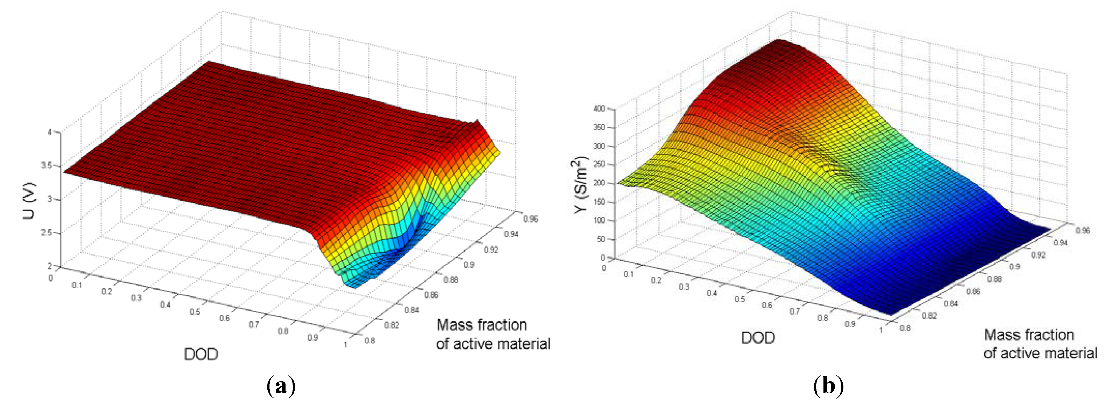
Figure 2. These results are given as the three-dimensional surface plots of
U and
Y as functions of
DOD and the mass fraction of active material in the cathode in
Figure 5. As shown in
Figure 5,
Y has a higher functional sensitivity to the mass fraction of active material than
U.
Figure 5.
Three-dimensional surface plots of (a) U; and (b) Y as functions of DOD and the mass fraction of active material in the cathode.
Figure 5.
Three-dimensional surface plots of (a) U; and (b) Y as functions of DOD and the mass fraction of active material in the cathode.
By using the values of
U and
Y in
Figure 5, the discharge capacities at the discharge rates of 0.1C, 0.5C, 1.0C, and 2.0C are estimated for compositions of the cathode ranging from 80% to 92.5% of the active material in the cathode, and the results are plotted in
Figure 6. At a discharge rate of 0.1C, the discharge capacity decreases monotonically with the mass fraction of the active material in the cathode for the range of cathode compositions investigated in this work. At discharge rates greater than 0.1C, the discharge capacity decreases as the mass fraction of active material in the cathode decreases up to 0.875. However, the discharge capacity increases as the mass fraction of active material in the cathode reaches 0.825, and it then decreases again as the mass fraction of the active material in the cathode decreases.
Figure 6.
(a) Discharge capacities with discharge rates ranging from 0.1C to 2.0C for various cathode compositions; and (b) three-dimensional surface plot of the discharge capacity as a function of the discharge C-rate and the mass fraction of active material in the cathode.
Figure 6.
(a) Discharge capacities with discharge rates ranging from 0.1C to 2.0C for various cathode compositions; and (b) three-dimensional surface plot of the discharge capacity as a function of the discharge C-rate and the mass fraction of active material in the cathode.
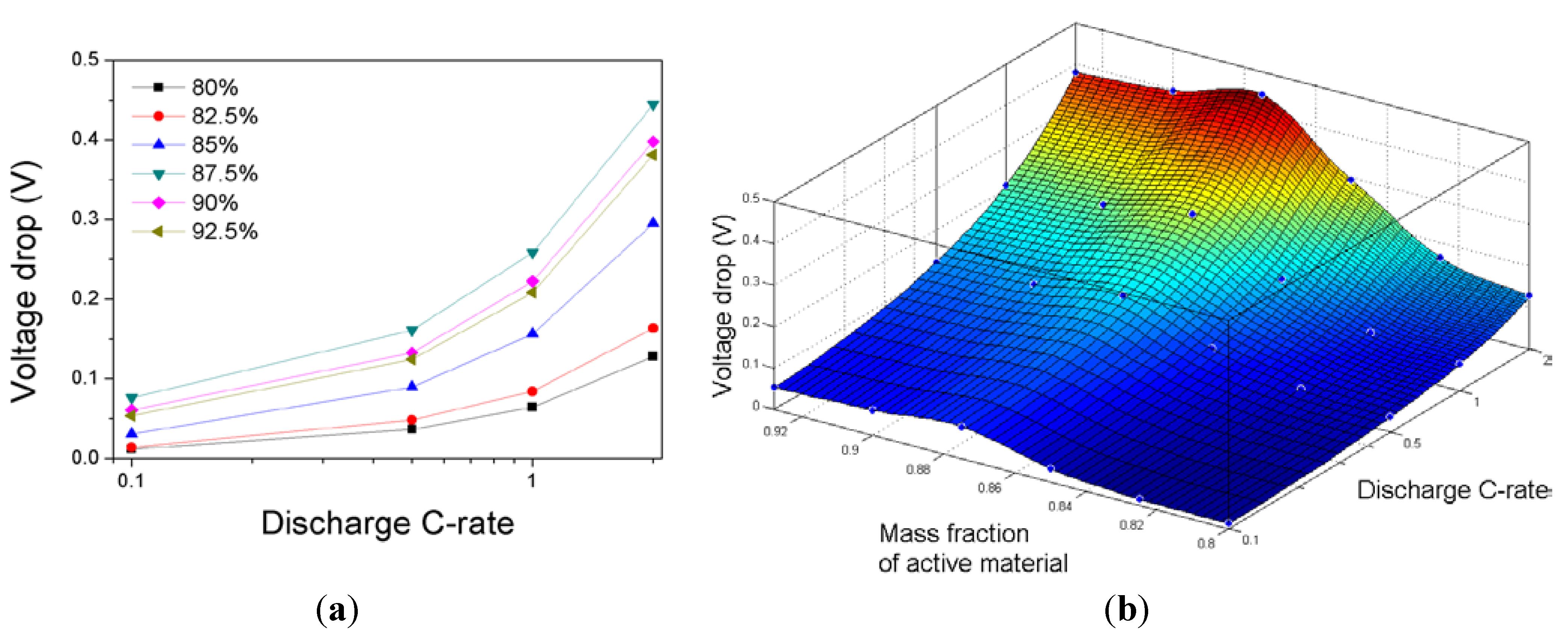
The battery cell voltage depends on many factors such as the discharge rate,
DOD, and cell chemistry. The cell voltage drops owing to an increase in
DOD from 0.2 to 0.8 with discharge rates ranging from 0.1C to 2.0C are calculated with the values of
U and
Y in
Figure 5 for various compositions of the cathode and are plotted in
Figure 7.
Figure 7.
(a) Voltage drops due to an increase in DOD from 0.2 to 0.8 with discharge rates ranging from 0.1C to 2.0C for various compositions of the cathode; and (b) three-dimensional surface plot of the voltage drop due to an increase in DOD from 0.2 to 0.8 as a function of the discharge C-rate and the mass fraction of active material in the cathode.
The voltage drops increase monotonically as the discharge rates increase; however, they increase as the mass fraction of the active material in the cathode increases up to 0.875, and they then decrease as the mass fraction of the active material in the cathode increases. Because the discharge capacity and the cell voltage drop owing to an increase in DOD exhibit highly nonlinear dependencies on the discharge C-rate and the mass fraction of active material in the cathode, it is necessary to develop an efficient modeling tool to estimate the effect of the cathode composition on the discharge behavior of a LFP battery cell. Modeling may save a considerable amount of time and money to identify the optimal composition of the electrodes, particularly when the battery performance depends nonlinearly on many factors through the limitless iterations performed using simulations.


