1. Introduction
With the deterioration of the environment and depletion of conventional resources, it has become imperative and advisable to search for alternative energy resources that are sustainable, clean and environmentally respectful. As a result, most industrialized countries have adopted policies to increase installed power with renewable energy power plants in order to comply with international environmental agreements. In particular, at the European Council in March 2007, the European Union endorsed a mandatory target of a 20% share of energy from renewable sources in overall community energy consumption by 2020. Also imposed on the Member States are individual targets in order to enable them to decide on their own, the preferred energy mix of alternative energy sources to fulfill this objective [
1].
Among renewable energy sources, wind power is undoubtedly the one that has experimented the greatest growth over recent years, turning into a base pillar of the energy system in many countries and, thus, becoming the true alternative to fossil fuels. As a result, the worldwide installed wind power capacity has increased considerably in these early years of the 21st century, and it is estimated that by 2013, installed wind power worldwide would amount to 318.0 GW, compared to 120.0 GW at the close of 2008 [
2].
In this regard, the principal feature of wind power concerning its integration into the grid is that it is not programmable. In contrast to conventional energy sources, wind power production cannot be specified beforehand, but depends on the incoming wind on various wind farms. Moreover, if wind power production is not known with sufficient accuracy, the power system regulators should make detailed schedule plans and set reserve capacity to prevent the possible fluctuation of this. To reduce the reserve capacity and increase the penetration of wind power, accurate forecasting of wind speed is needed [
3].
Numerous studies about wind speed prediction or wind power prediction can be found in the scientific literature. The calculation of wind power production is carried out by means of the relationship between electric power production and wind speed, obtained empirically for the park itself or using the power curve provided by the manufacturer of the wind turbine. In addition to the variable of prediction, the forecasting models are classified according to the prediction horizon, the forecasting methodology and the type of data.
Short-term predictions are usually based on time series analysis, from simpler (autoregressive models, linear multiple regression and persistence) to complex structures (computational fluid dynamic, neural networks and fuzzy logic). Taylor
et al. [
4] compared the methods. Lei
et al. [
5] gave a survey on the general background and developments in wind speed and wind power forecasting. This study is completed by consulting Foley
et al. [
6], who gave a review of the current methods and advances.
It is well known that artificial neural networks (ANNs) are used to predict wind parameters: hourly wind speed, wind directions, wind farm production,
etc. By way of example, the following references are available, which apply ANN-based models [
7,
8,
9,
10,
11,
12,
13,
14]; hybrid methods can be found in [
15,
16,
17,
18,
19]. The availability of many measuring points of wind speed might be conducive to the performance of works, like [
20,
21]. Bilgili
et al. [
22] made a study to predict the monthly mean wind speed in the eastern Mediterranean region of Turkey using high-quality measurements.
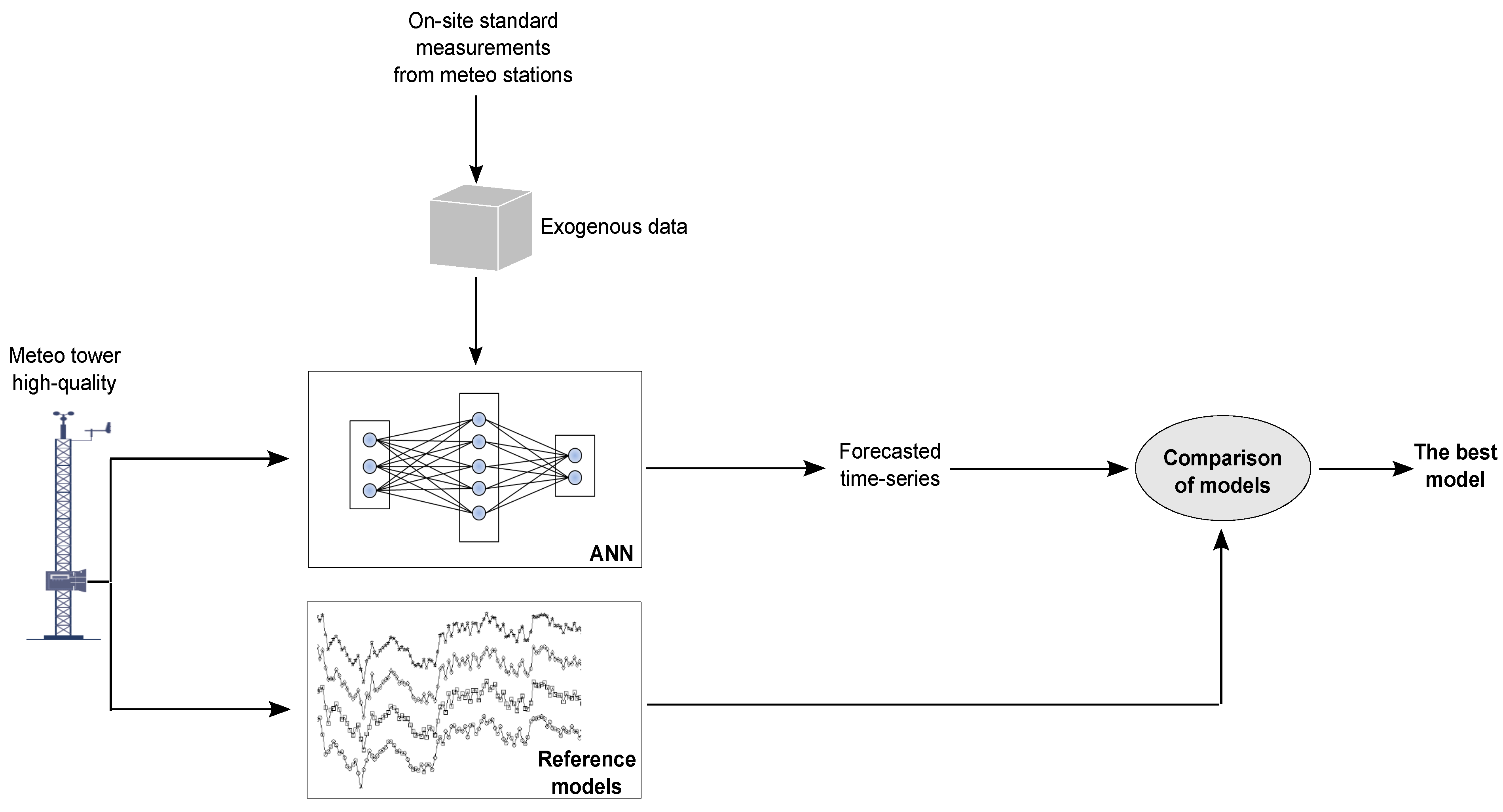
This work uses exogenous data, from standard weather stations in the surroundings of the target area, to improve short-term forecasting of ANNs. The value-added novelty of the paper lies in the fact that these stations are not yet considered by the World Meteorological Organization [
23]. In this sense, these papers establish a scientific proposal and a method for them to be included [
24,
25].
The paper is organized in the following way:
Section 2 presents the region and the raw data from the on-site equipment;
Section 3 summarizes the theoretical framework; the experimental procedure is outlined in
Section 4; and results are analyzed in
Section 5; finally, conclusions are drawn in
Section 6.
2. Data Description
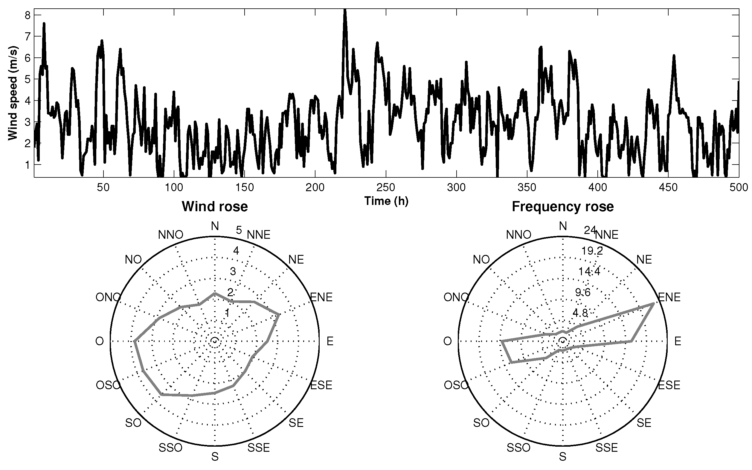
The target 20 m-high wind measurement tower, located at Universal Transverse Mercator coordinates (294,284.4175161) in Northern Andalusia (Peñaflor, Sevilla, Spain), acquires data at 10 min intervals, covering the period from September 2007 to August 2008.
Table 1 lists the main characteristics of the measured variables.
Table 1.
Main characteristics of the target station.
Table 1.
Main characteristics of the target station.
| Variable | Speed at 20 m (m/s) | Temperature (C) | Pressure (mb) | Density (kg/m) |
|---|
| Mean | 2.75 | 17.89 | 1010.54 | 1.2108 |
| Standard Deviation | 0.60 | 7.78 | 5.70 | 0.0344 |
| Max | 15.70 | 41.20 | 1027.00 | 1.2863 |
| Min | 0.40 | 1.40 | 983.00 | 1.1162 |
| Turbulence index | 0.22 | - | - | - |
| Calm | 18.12% | - | - | - |
Figure 1 shows the wind singularities at the target station through a wind speed graph, and the frequency and speed rose (only 500 records are displayed for better visualization).
Figure 1.
Wind characteristics at the target station.
Figure 1.
Wind characteristics at the target station.
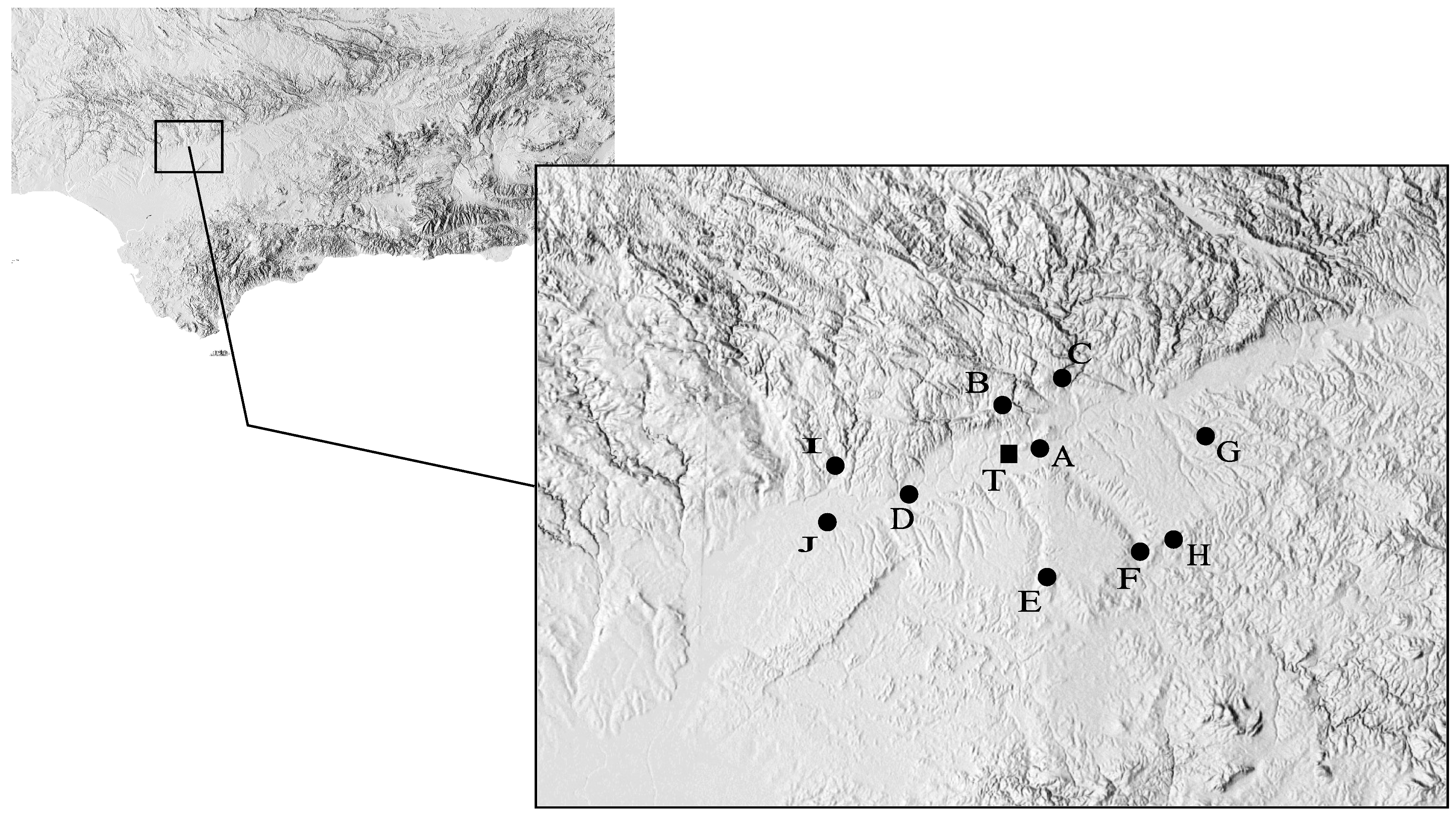
To improve predictions, the ten closest stations have been selected within a radius of 40 km, and initially conceived to measure agriculture variables (Andalusian agriculture-climate information network [
26]), providing hourly measurements. Wind records are not reliable enough, because most of them are located in the open air, being highly affected by obstacles (the anemometer’s height is 2 m).
Figure 2 shows the location of the target and reference stations.
Figure 2.
Map of the studied zone. T = target station.
Figure 2.
Map of the studied zone. T = target station.
Table 2 summarizes the geographical coordinates, average wind speed, distances and correlation coefficients of the stations with respect to the target. Note that the order shown in the
Table 2 is from lowest to highest separation distance relative to the target station.
Table 2.
Information of the used stations in this study.
Table 2.
Information of the used stations in this study.
| ID | Location | Latitude | Longitude | Altitude (m) | Distance (km) | Mean wind speed (m/s) | Correlation coefficient |
|---|
| (T) | Peñaflor | 37.71 | −5.35 | 42 | 0.0 | 2.75 | 1.00 |
| (A) | Palma del Río | 37.68 | −5.28 | 57 | 6.41 | 0.87 | 0.67 |
| (B) | La Puebla de los Infantes | 37.79 | −5.41 | 350 | 9.56 | 0.75 | 0.62 |
| (C) | Hornachuelos | 37.72 | −5.16 | 157 | 16.64 | 1.4 | 0.68 |
| (D) | Lora del Río | 37.66 | −5.54 | 68 | 17.69 | 1.66 | 0.66 |
| (E) | La Luisiana | 37.53 | −5.23 | 188 | 22.64 | 1.35 | 0.63 |
| (F) | Écija | 37.59 | −5.08 | 125 | 26.99 | 1.77 | 0.63 |
| (G) | Guadalcázar | 37.72 | −5.01 | 173 | 30.14 | 0.91 | 0.71 |
| (H) | Écija CA | 37.51 | −5.09 | 130 | 31.05 | 2.43 | 0.58 |
| (I) | Villanueva del Río y Minas | 37.61 | −5.68 | 38 | 31.34 | 1.21 | 0.62 |
| (J) | Tocina | 37.61 | −5.71 | 22 | 34.24 | 1.24 | 0.52 |
4. Development of the Proposed Models
After the experimental procedure has been explained in
Section 3, the reference models (persistence and ARIMA model) are assessed using the wind speed time series acquired at the target station (the wind speed in Peñaflor).
The implementation of the persistence model does not present any problems. However, the ARIMA model needs preliminary actions to establish the order
p,
d and
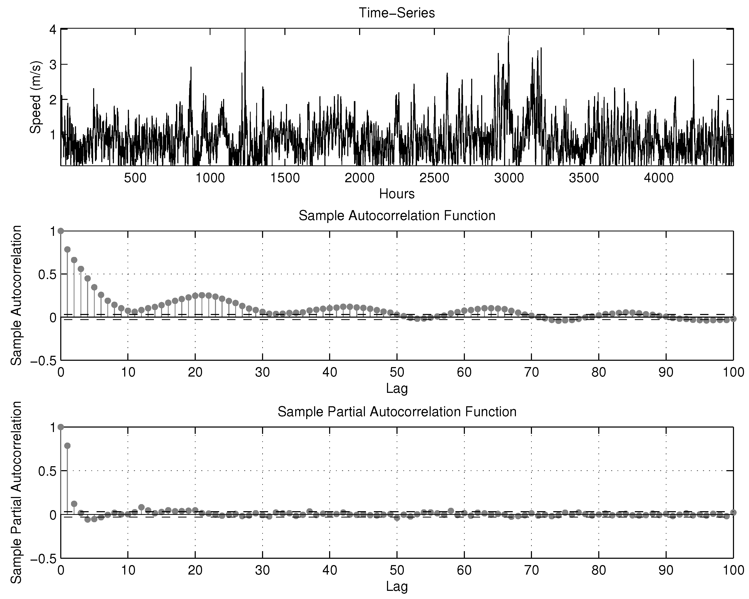
q which best fit the target time series. The Box-Jenkins methodology is adopted to identify these parameters. In the Box-Jenkins methodology, a differencing approach is used to stabilize the original data, and both an autocorrelation function (ACF) and a partial autocorrelation function (PACF) are utilized to decide the autoregressive or moving average component, which should be included in the ARIMA model. The choice of the appropriate values of the model is based on the ACF and PACF characteristics shown in
Table 3. With this goal, the autocorrelation coefficients and the partial autocorrelation coefficients are evaluated and depicted in
Figure 8.
Table 3.
Autocorrelation patterns of autoregressive integrated moving average (ARIMA) models. ACF: autocorrelation function; PACF: partial autocorrelation function; AR: autoregressive model; MA: moving average model; and ARMA: autoregressive-moving-average model.
Table 3.
Autocorrelation patterns of autoregressive integrated moving average (ARIMA) models. ACF: autocorrelation function; PACF: partial autocorrelation function; AR: autoregressive model; MA: moving average model; and ARMA: autoregressive-moving-average model.
| Process | ACF | PACF |
|---|
| AR(p) | Infinite, but convergent | Finite: cut off at lag p |
| MA(q) | Finite: cut off at lag q | Infinite, but convergent |
| ARMA (p,q) | Infinite: exponential and/or sine-cosine wave decay | Infinite: exponential and/or sine-cosine wave decay |
The autocorrelation coefficients shown in
Figure 8 decay as the time-lag increases, but they have positive correlations for many time-lags. This conveys the idea that one order of differentiating is needed [
36].
Figure 8.
Time series wind speed, autocorrelation function (ACF) and partial autocorrelation function (PACF) plots at Peñaflor.
Figure 8.
Time series wind speed, autocorrelation function (ACF) and partial autocorrelation function (PACF) plots at Peñaflor.
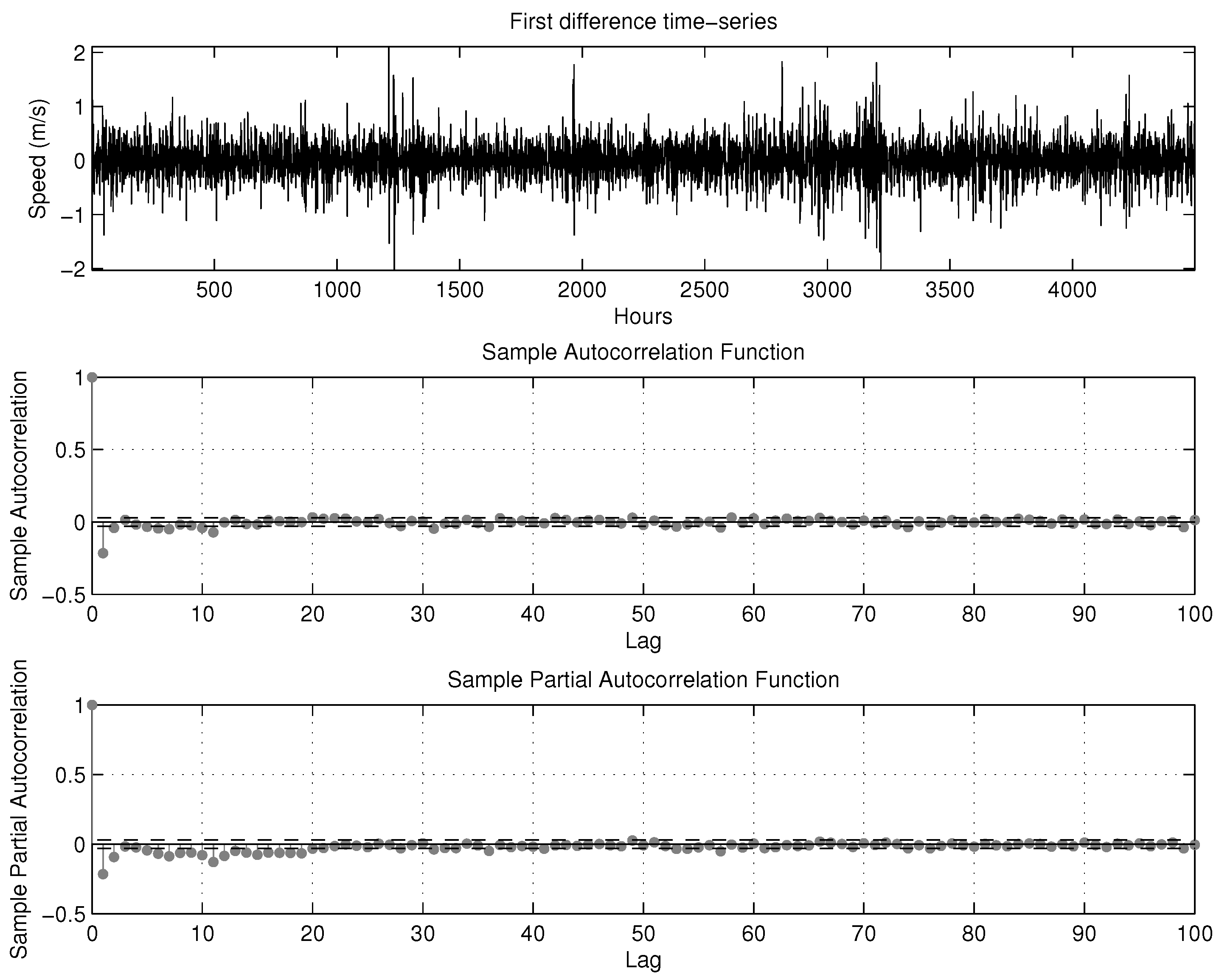
Figure 9 shows the prospective results of the model from the first derivative time series. The selection of three potential models has been established based on the inspection of this graph:
PACF cuts beyond the second lag. According to the above explanations, ARIMA (2,1,0) should be selected;
ACF decays in the second lag. Thus, ARIMA (0,1,2) is selected;
ACF and PACF have a decreasing and oscillating phenomenon that begins in the second lag. Consequently, ARIMA (2,1,2) has been selected.
Figure 9.
Differentiated original time series wind speed, ACF and PACF plots at Peñaflor.
Figure 9.
Differentiated original time series wind speed, ACF and PACF plots at Peñaflor.
In the estimation process, the errors of each model [ARIMA (2,1,0), ARIMA (0,1,2), and ARIMA (2,1,2)] have been calculated along with their parameters attending to the maximum likelihood paradigm. The best model is selected with the help of Akaike and Bayesian information criteria [
37]: ARIMA (2,1,0) with coefficients
0.2352 and
0.0922.
The last step of the ARIMA process is the diagnosis testing. In this step, the assumptions on the residuals are validated, so that the model can be used to forecast.
For the predictor, MLR, which is based on a statistical linear model, no tuning parameters are needed, and the inputs used for training and validation are the same as those used in the ANNs.
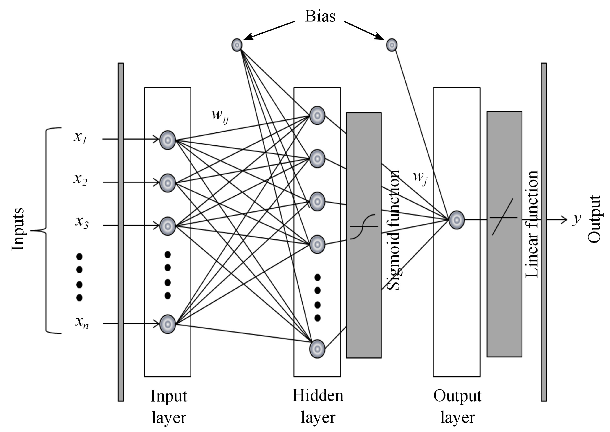
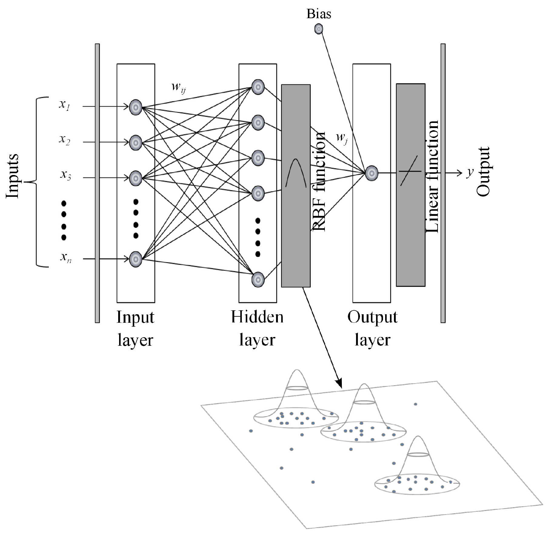
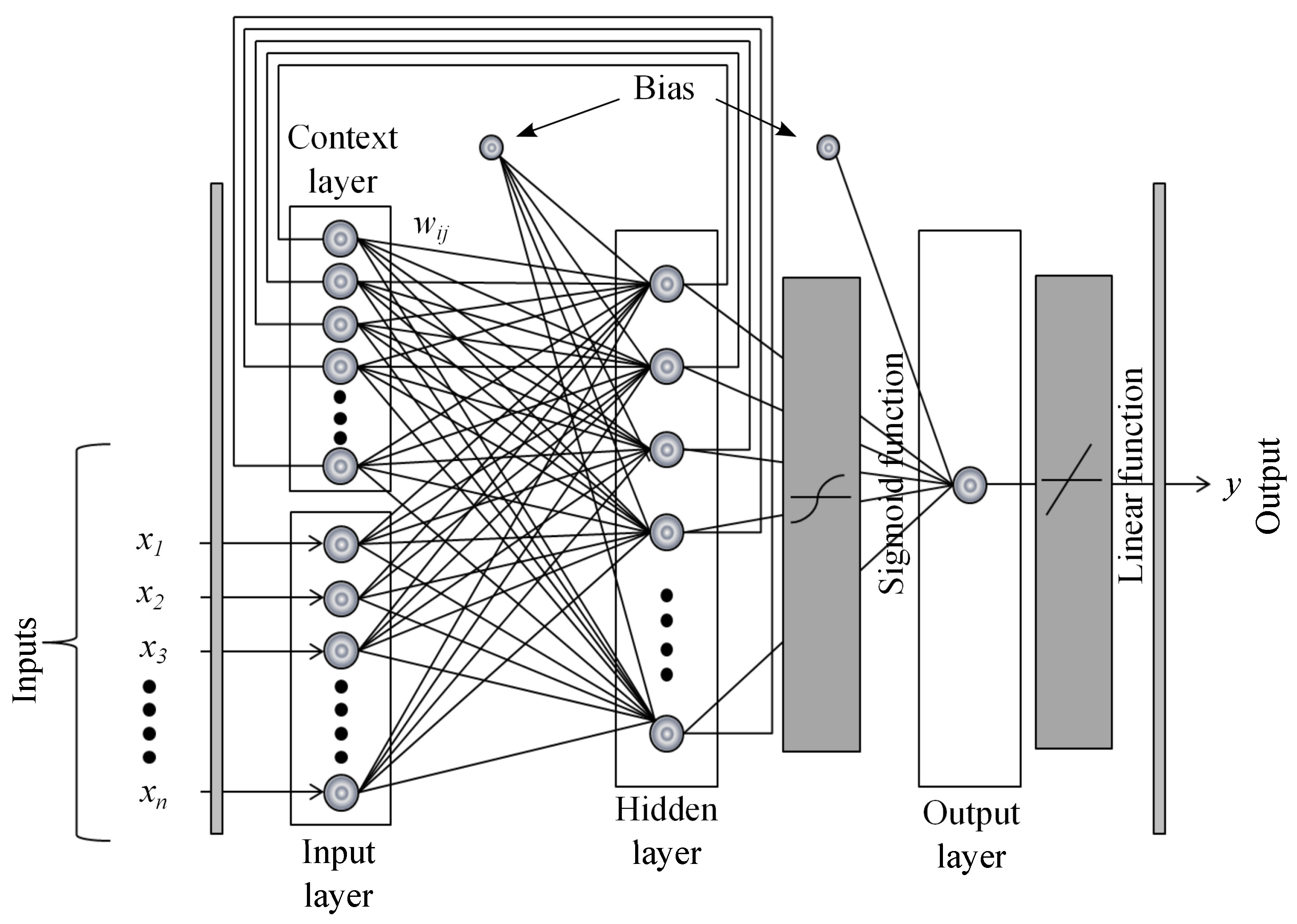
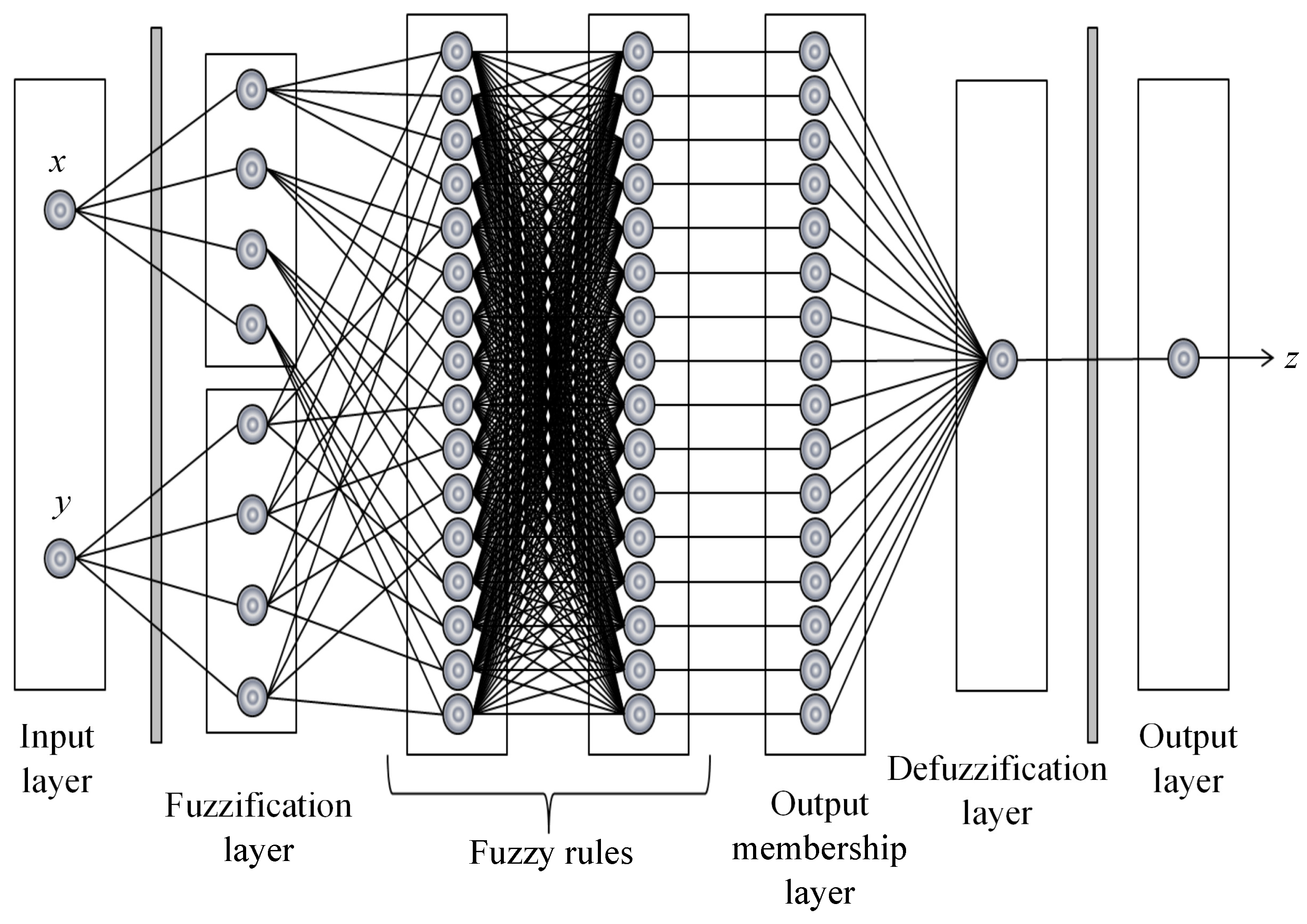
The following models are tested in this paper: backpropagation network with one and two hidden layers (BP1 and BP2), RBF network, Elman neural network (ELM) and ANFIS. The following premises are considered:
the reference stations in
Section 2 have been used as exogenous variables to improve the prediction;
data are normalized, so that they are in the interval [−1, 1] for a faster computation;
the dataset was divided into three subsets: training, evaluation and test sets. The training and validation sets, with 70% and 15% of the data, respectively, were used for ANN model building; and the third set, with the last 15%, was used to test the predictive power of a model on the out-of-sample set. The building model is performed in two phases: the first one uses the training set to obtain the parameters for non-linear predictors; and, the second phase uses the validation set to choose the optimum;
the training of the tested networks is carried out until the validation error starts increasing. At this point, we stop the training, and the performance of the network is measured in the test. One hundred experiments have been launched for each model in order to achieve statistically meaningful results which rule out the random factors influencing the ANN, and we keep the best results.
Hereinafter, we detail the particularities of the models.
Table 4 collects parameters, corresponding to the network architecture and activation functions of neural networks.
Table 4.
Parameters of the network models used. BP: backpropagation; RBF: radial basis function; ELM: Elman neural network.
Table 4.
Parameters of the network models used. BP: backpropagation; RBF: radial basis function; ELM: Elman neural network.
| Parameter | BP1 | BP2 | RBF | ELM |
|---|
| Hidden layers | 1 | 2 | 1 | 1 |
| Neurons in hidden layer 1 | [4,10] | [4,10] | [1,150] | [4,10] |
| Neurons in hidden layer 2 | - | - | [2,5] | - |
| Transfer function (TF) | Sigmoid | Sigmoid | Gaussian | Sigmoid |
| TF output layer | Linear | Linear | Linear | Linear |
| Training algorithm | Levenberg Marquardt | Levenberg Marquardt | k-means | Gradient descent |
| Spread | - | - | [1,20] | - |
The rule to select the range of neurons in the hidden layers for BP1, BP2 and ELM models is as follows. The number of neurons in the first hidden layer is the mean of the neurons between the input and output layers, and the number of neurons in the second hidden layer is one half of the neurons in the first hidden layer [
38]. As the maximum number of inputs is eleven and the number of outputs is one, the ranges for the first and second hidden layers are [4,10] and [2,5], respectively, as shown in
Table 4.
For the RBF model, we must specify the appropriate value of the Gaussian Kernel width or spread. The higher the value assigned to this parameter, the smoother the approximation function. Too large a spread means a lot of neurons are required to fit a fast-changing function. Conversely, too small a spread means many neurons are required to fit a smooth function, and the network might not generalize well. Different training architectures were analyzed depending on the spread and the number of hidden neurons. We specify the first variable in the range of [1,20] and the second variable between 1 and 150 neurons.
A total of 500 ANFIS models have been designed considering different combinations of inputs and rules. Similar to ANNs, the input space is divided into two groups: one with 70% of the data for the training and the other with the remaining 30% for validation of the model.
Table 5 resumes the parameters used to specify the assessed ANFIS models.
Table 5.
ANFIS parameters. MF: member function.
Table 5.
ANFIS parameters. MF: member function.
| Parameters | Value | Function |
|---|
| Input MFs | 8 | - |
| Number of input MFs | [3,7] | - |
| Output MFs | - | Linear |
| Optimization method | - | Hybrid |
| Epochs | 500 | - |
In all tested models (ANNs and MLR), the wind speed and direction data of the reference stations have been applied as exogenous variables. The prediction of the objective variable at an instant,
t, is done using the exogenous data of a previous time (
1). Then, data are presented in an autoregressive matrix. For example, the autoregressive matrix shown in
Table 6 is associated with wind speed prediction supported by four exogenous variables.
Table 6.
Example of the autoregressive matrix.
Table 6.
Example of the autoregressive matrix.
| Target | Target | Exogenous | Exogenous | Exogenous | Exogenous |
|---|
| variable | variable | variable 1 | variable 2 | variable 3 | variable 4 |
|---|
| | | | | |
| | | | | |
| | | | | |
| | | | | |
| | | | | |
| | | | | |
| | | | | |
| ⋮ | ⋮ | ⋮ | ⋮ | ⋮ | ⋮ |
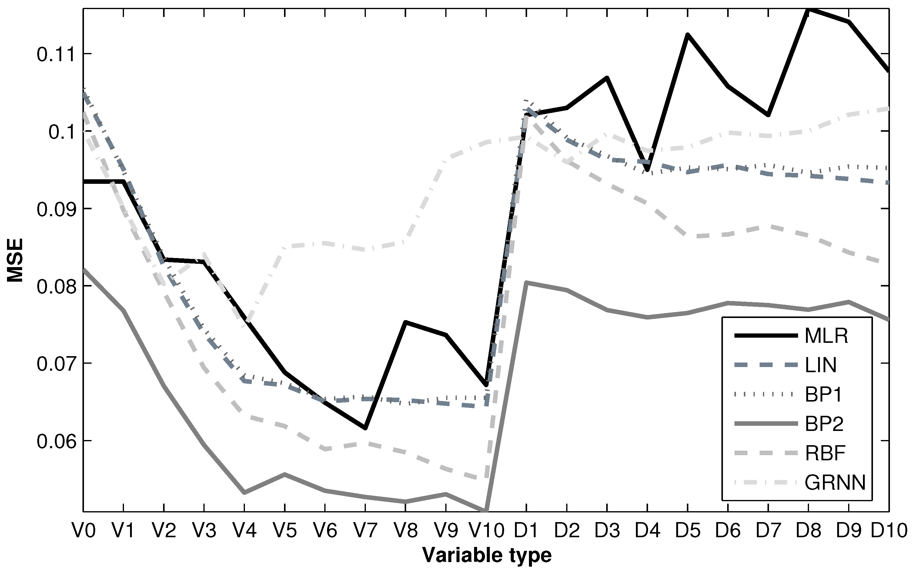
Figure 10 shows the evolution of the performance of the models based on the MSE criterion and the type of variable used. As can be seen, first, the simulations begin without exogenous variables, and then, they are progressively inserted from one to ten stations (from highest to lowest correlation). In principle, simulations only consider the wind speed time series at each station as exogenous variables; then, both wind speed and direction are applied. On the basis of a visual assessment, it is evident that the insertion of wind direction data does not lead to the improvement of the performance of the models; so henceforth, only the wind speed data for each station will be taken into account as exogenous variables. Each model’s performance is summarized by the former four quality indexes.
Figure 10.
Evolution of the performance of the models.
Figure 10.
Evolution of the performance of the models.
5. Results
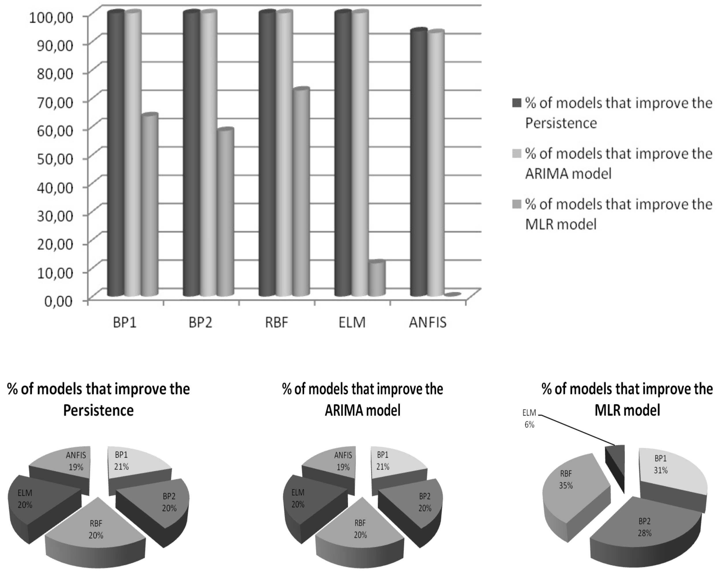
The number of models tested in this work amounts to more than 3200 configurations, attending to their typology (BP, RBF, ELM or ANFIS), tuning parameters and exogenous variables used in the simulations: 98.72% of them are better than persistence, 98.60% are better than the ARIMA (2,1,0) model and 41.30% are better than the MLR model. For the sake of comparison,
Table 7 shows the results of the quality indexes on the test set obtained by the ten best models that generated the smallest MSE and also the values associated with the reference models [persistence, ARIMA (2,1,0) and MLR]. Note that these results are ordered in terms of the MSE criterion, because this is the objective function adopted in the learning process of the models.
Table 7.
Parameters and results achieved on the test set by the reference models vs. the ten best models. IOA: index of agreement; MAE: mean absolute error; MAPE: mean absolute percentage error; and MSE: mean squared error.
Table 7.
Parameters and results achieved on the test set by the reference models vs. the ten best models. IOA: index of agreement; MAE: mean absolute error; MAPE: mean absolute percentage error; and MSE: mean squared error.
| Model | Exogenous speed | | | Spread | R | IOA | MAE | MAPE | MSE |
|---|
| Persistence | - | - | - | - | 0.7779 | 0.8800 | 0.9191 | 48.8027 | 1.5495 |
| ARIMA (210) | - | - | - | - | 0.7807 | 0.8809 | 0.9069 | 49.8449 | 1.4636 |
| MLR | 9 | - | - | - | 0.8777 | 0.9332 | 0.6854 | 39.6604 | 0.7866 |
| BP1 | 6 | 5 | - | - | 0.8917 | 0.9400 | 0.6516 | 38.9846 | 0.6735 |
| BP2 | 7 | 10 | 2 | - | 0.8825 | 0.9323 | 0.6981 | 44.1851 | 0.6737 |
| RBF | 8 | 86 | - | 5 | 0.9021 | 0.9448 | 0.6429 | 38.4153 | 0.6756 |
| RBF | 10 | 116 | - | 6 | 0.8932 | 0.9422 | 0.6546 | 40.7415 | 0.6762 |
| RBF | 9 | 93 | - | 5 | 0.8945 | 0.9435 | 0.6348 | 36.9671 | 0.6804 |
| BP1 | 10 | 10 | - | - | 0.8885 | 0.9384 | 0.6433 | 37.0831 | 0.6815 |
| BP2 | 8 | 9 | 5 | - | 0.8919 | 0.9408 | 0.6484 | 38.0996 | 0.6825 |
| BP1 | 5 | 4 | - | - | 0.8945 | 0.9395 | 0.6489 | 40.9397 | 0.6922 |
| BP2 | 7 | 7 | 5 | - | 0.8924 | 0.9390 | 0.6418 | 43.2729 | 0.6949 |
| RBF | 7 | 56 | - | 4 | 0.8965 | 0.9412 | 0.6466 | 39.5675 | 0.6987 |
As shown in
Table 7, the results of the models supported by low-quality stations significantly improve the reference models: the persistence, ARIMA (2,1,0) and MLR. The best of all the models tested is a backpropagation network with one hidden layer (BP1) and five neurons within the hidden layer. There are seven inputs for this model: one of them is the wind speed of the target station, and the rest are exogenous speed values registered at the six closest stations. This model reduces the MAE and MSE with respect to the persistence model by 29.10% and 56.54%, respectively. The percentages of improvement over the ARIMA (2,1,0) model are 28.15% and 53.99%, and the percentages of improvement over the MLR model are 4.93% and 14.38%. None of the ten best models uses directions as exogenous variables, indicating that this information is not significant.
Once the analysis based on quality indexes has been completed, a multiple comparison procedure is carried out with the best models selected in the
Table 7. As was discussed in
Subsection 3.2, the analysis is composed of the parametric test (ANOVA) and the
Bonferroni adjustment.
Table 8 shows the results, in terms of MSE, obtained for each of the ten best models selected in
Table 7. One hundred experiments were performed for statistical analysis. As illustrated in
Table 8, the model,
ExogVar, proves the robustness and capacity for enhancing the prediction errors of the reference models. This is confirmed by means of the statistical tests (ANOVA and Bonferroni’s test).
Table 8.
Evaluation of MSE for the 10 best models. The results are averaged over 100 runs.
Table 8.
Evaluation of MSE for the 10 best models. The results are averaged over 100 runs.
| Model | MSE Mean | SD | Min | Max |
|---|
| 0.8647 | 0.0683 | 0.6735 | 1.0535 |
| 1.0054 | 0.4392 | 0.6737 | 2.9510 |
| 0.8425 | 0.0555 | 0.6756 | 0.9659 |
| 0.8211 | 0.0611 | 0.6762 | 0.9600 |
| 0.8717 | 0.0591 | 0.6804 | 0.9944 |
| 0.8670 | 0.0655 | 0.6815 | 1.0379 |
| 0.8700 | 0.0687 | 0.6825 | 1.0104 |
| 0.8884 | 0.0619 | 0.6922 | 1.0545 |
| 0.8789 | 0.0641 | 0.6949 | 1.0012 |
| 0.9008 | 0.0641 | 0.6987 | 1.0367 |
Table 9 shows the models, the corresponding mean errors and the Bonferroni’s test results. The order shown in this table is from lowest to highest MSE mean. As we can see, Model 1 belongs to the group of models that do not have significantly different means. Therefore, this model should be selected coinciding with the results obtained in
Table 7.
Table 9.
Bonferroni’s test results.
Table 9.
Bonferroni’s test results.
| Model | Error mean | Models not significantly different |
|---|
| 4 | 0.8211 | 4 3 6 1 7 5 9 8 10 |
| 3 | 0.8425 | 4 3 6 1 7 5 9 8 10 |
| 6 | 0.8607 | 4 3 6 1 7 5 9 8 10 |
| 1 | 0.8647 | 4 3 6 1 7 5 9 8 10 |
| 7 | 0.8700 | 4 3 6 1 7 5 9 8 10 |
| 5 | 0.8717 | 4 3 6 1 7 5 9 8 10 |
| 9 | 0.8789 | 4 3 6 1 7 5 9 8 10 |
| 8 | 0.8884 | 4 3 6 1 7 5 9 8 10 |
| 10 | 0.9008 | 4 3 6 1 7 5 9 8 10 2 |
| 2 | 1.0054 | 10 2 |
As mentioned before, results show that the best model using the two selection processes (quality indexes and statistical analysis), called ExogVar, enhances the effectiveness of the forecast through exogenous information received from agricultural measurement stations.
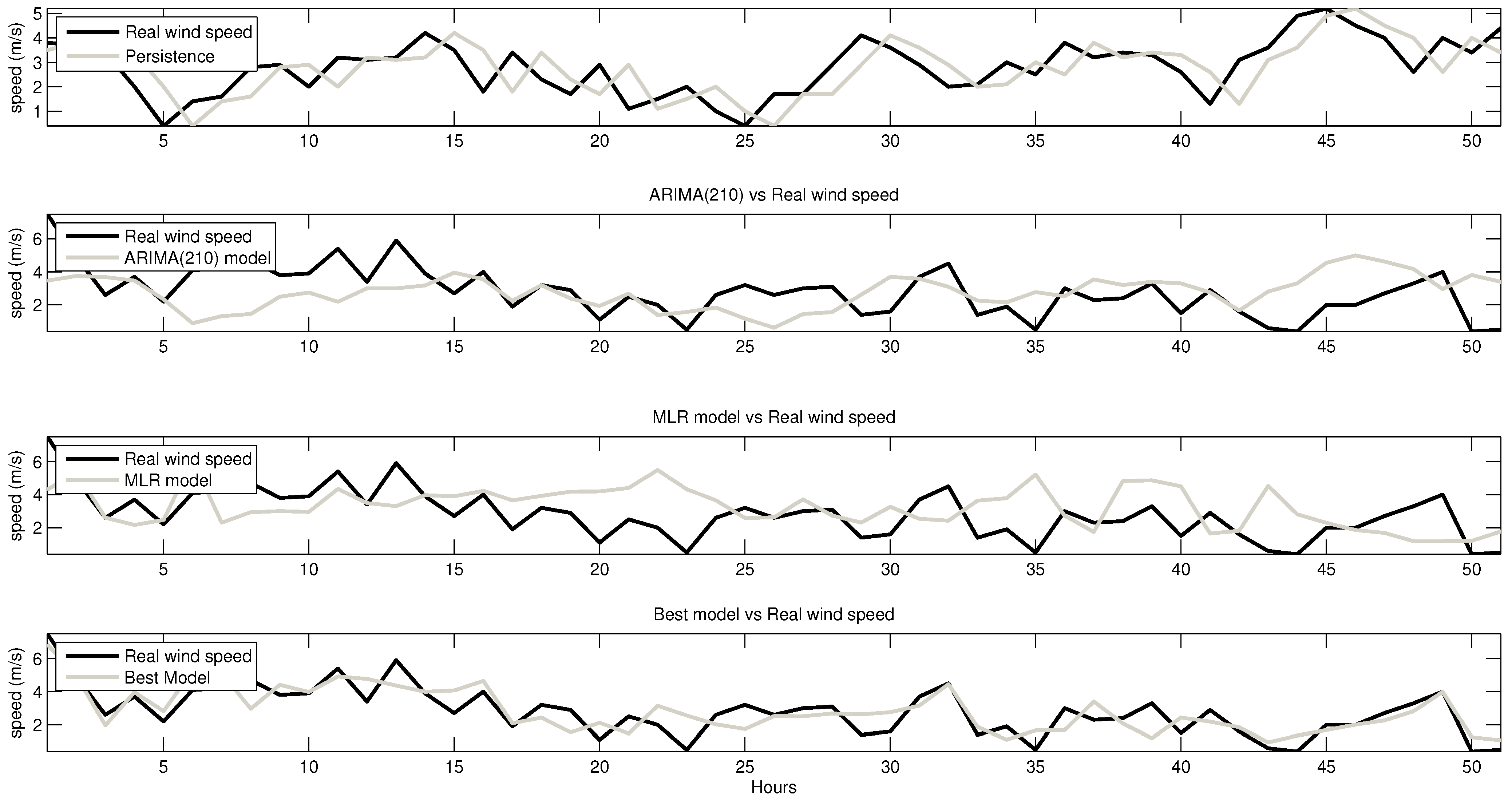
Figure 11 depicts the performance of the best model, i.e., the one shown in
Table 7 with the best quality indexes. The same graph also shows the three reference models (persistence, ARIMA and MLR). The data belong to the test set, and only 50 h are shown for a better visualization of the results. As expected, the time series by the best model based on the ANN is clearly more accurate than the reference ones.
Figure 11.
Original time series and forecasted data with the best obtained model.
Figure 11.
Original time series and forecasted data with the best obtained model.
The overall improvements obtained by the selected neural network models on the reference models are shown in
Figure 12. In addition, the improvements of the models are also depicted, ranked by percentage.
Figure 12.
Overall improvements of the models.
Figure 12.
Overall improvements of the models.
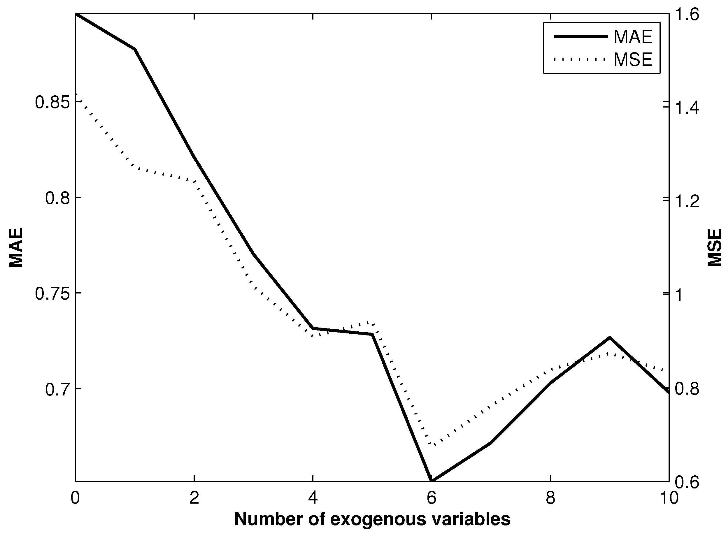
Once the best model has been selected through the two procedures, it is assessed in terms of the number of exogenous variables used. Hence, we started using the time series registered in the target as the sole input (without exogenous variables). Then, one by one, the exogenous time series were used to evaluate their benefits. As is possible to see in
Figure 13, the MAE and MSE indexes are improved by the inclusion of exogenous measurements. The achievement is optimum using the speed registers from the six nearest stations.
Figure 13.
Evolutions of the mean absolute error (NAE) and mean squared error (MSE) errors obtained by the best model in the function of the exogenous variables used.
Figure 13.
Evolutions of the mean absolute error (NAE) and mean squared error (MSE) errors obtained by the best model in the function of the exogenous variables used.
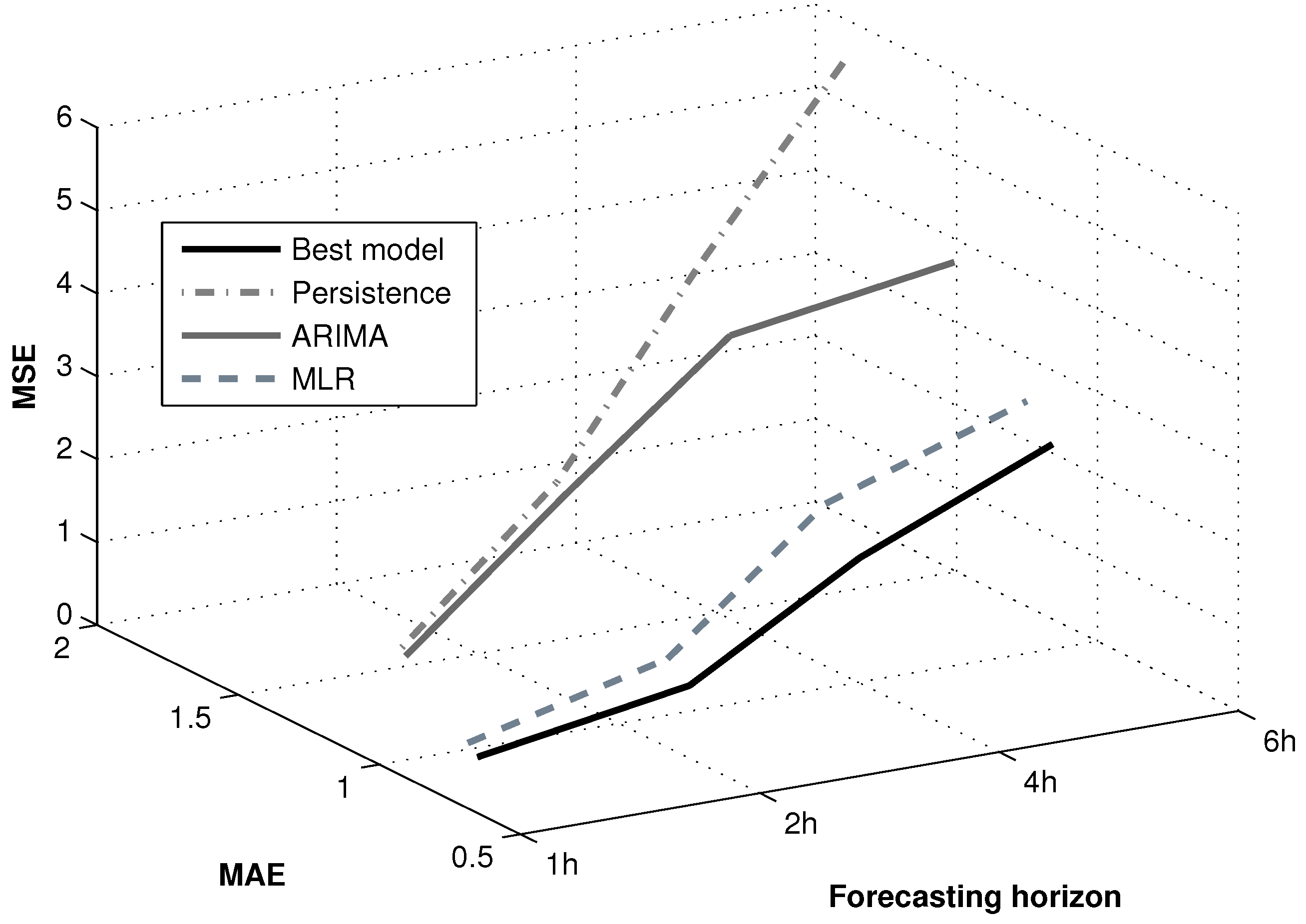
Finally, and to complete this study, the best architecture (BP1: five hidden neurons) is analyzed in the function of the forecasting horizon. The assessment is based on the forecasting horizons of 1, 2, 4 and 6 h. As
Figure 14 shows, the MSE and MAE indexes get worse as the forecasting horizon progresses, although the best model still exceeds the three reference models.
Figure 14.
Evolutions of the MAE and MSE errors obtained by the best model in the function of the forecasting horizon.
Figure 14.
Evolutions of the MAE and MSE errors obtained by the best model in the function of the forecasting horizon.
6. Conclusions
The main contribution of this work is that wind speed predictions in a target station can be significantly improved by the use of low-quality wind data acquired at surrounding agriculture measurement stations. The originality of this study concerns the application of stations which are generally excluded from wind assessment. These low-quality data are excluded because of their low reliability, and the measurements locations are not optimal.
In the present case, the best model to perform 1 h-ahead prediction is a backpropagation network with one hidden layer and five neurons. This model uses six exogenous speed values and meaningfully improves the three witness models according to four quality indexes: ρ, IOA, MAE and MSE. The main enhancements are more visible in MAE, which achieves a value of 0.65 m/s, and MSE with 0.67 m/s. The percentages of improvement with respect to the reference models are 29.10% and 56.54% for the persistence, 28.15% and 53.99% for the ARIMA (2,1,0) and 4.93% and 14.38% for the MLR model.
In summary, it might be concluded that data from low-quality stations, which are ruled out because of low reliability and do not achieve the World Meteorological Organization requirements, provide useful information for the control of a wind farm. This information optimizes the control in two aspects: short-term predictions and wind farm maintenance. This fact could benefit the insertion of this renewable energy source into areas where the wind energy represents a high percentage of the total electric power.


 ,
, 


