Altering Kinetic Energy Entrainment in Large Eddy Simulations of Large Wind Farms Using Unconventional Wind Turbine Actuator Forcing ^†

Abstract

In this study, horizontally periodic large eddy simulations (LES) are utilized to study turbulent atmospheric boundary-layer flow over wind turbines in the far-downstream portion of a large wind farm where the wakes have merged and the flow is fully developed. In an attempt to increase power generation by enhancing the mean kinetic energy (MKE) entrainment to the wind turbines, hypothetical synthetic forcing is applied to the flow at the turbine rotor locations. The synthetic forcing is not meant to represent any existing devices or control schemes, but rather acts as a proof of concept to inform future designs. The turbines are modeled using traditional actuator disks, and the unconventional synthetic forcing is applied in the vertical direction with the magnitude and direction dependent on the instantaneous velocity fluctuation at the rotor disk; in one set of LES meant to enhance the vertical entrainment of MKE, a downward force is prescribed in conjunction with a positive axial velocity fluctuation, whereas a negative axial velocity fluctuation results in an upward force. The magnitude of the forcing is proportional to the instantaneous thrust force with prefactors ranging from 0.1 to 1. The synthetic vertical forcing is found to have a significant effect on the power generated by the wind farm. Consistent with previous findings, the MKE flux to the level of the turbines is found to vary along with the total power produced by the wind turbine array. The reverse strategy of downward forcing of slow axial velocity flow is found to have almost no effect on the power output or entrainment. Several of the scenarios tested, e.g., where the vertical force is of similar magnitude to the horizontal thrust, would be very difficult to implement in practice, but the simulations serve the purpose of identifying trends and bounds on possible power increases from flow modifications through action at the turbine rotor.

1. Introduction

To meet the world’s growing energy demands while minimizing the emission of greenhouse gases, developers around the world have installed over 35 GW of wind energy capacity in the year 2013 [1]. These new wind turbines are often installed in clusters or arrays to take advantage of available land and infrastructure, but when wind turbines are placed in proximity to one another, the wakes of upstream turbines can reduce the available energy to nearby downstream turbines, while simultaneously increasing undesirable small-scale turbulent fluctuations (see e.g., [2,3,4,5,6]). The authors in [7,8,9,10,11] provide examples of optimization strategies, which consider the trade-off between efficient land use and minimization of turbulent wake interaction. Any modification to wind farm design that can offset this detrimental “wake effect” has the potential to improve the performance and lifetime of these wind farms, thereby reducing the cost of energy.

Previous research has shown that increasing the distance between wind turbines is beneficial, as it allows for wake recovery (e.g., [3,8,12]), but achieving this separation is especially difficult when the direction of the wind changes significantly over the course of the year; an efficient layout for one wind direction could be extremely undesirable for another wind direction (see e.g., the design of the Middelgrunden wind farm). Designing optimal layouts for a wind farm is one approach to addressing this issue (see e.g., [13,14]); changing the design or operation of the wind turbine itself is another. Specifically, we are interested in the question of whether wind turbines could operate to enhance wake recovery and, therefore, benefit downstream turbines. One operational approach might be to direct the wake horizontally, right or left, while another might be to enhance the kinetic energy entrainment by directing the wake vertically, up or down [15,16]. In this paper, we explore the latter approach and perform a proof of concept study, a “what if” numerical experiment to test one of many possible approaches to turbine redesign.

Turbulent transfer of kinetic energy from above replenishes energy extracted by the turbine wakes, and this kinetic energy entrainment becomes the limiting factor in wind farm performance for very large wind farms [12,17,18,19,20,21]. The entrainment of kinetic energy, and the means to modify it, is the focus of the present study. A wind turbine operator might attempt to alter this transfer by tilting the rotor upward or downward according to the instantaneous measured velocity. Adapting the rotor operation (e.g., via tilting, yawing, turning the blades; see [22]) to induce a downward force when encountering high-speed streamwise flow, for example, has the potential to enhance the already existing turbulent transfer. This effect would be especially pronounced for very large wind farms in which the atmospheric boundary layer has found an equilibrium with the wind turbines; in this state, the power tends to level off (as seen in [2]) as the flow becomes well mixed, and the turbine wakes are less able to recover by horizontal expansion. We explore the question of whether modifications to individual wind turbine aerodynamic characteristics, represented here in an exploratory attempt by synthetic vertical forcing at the turbine rotor, could affect the overall vertical kinetic energy flux in very large wind turbine arrays. The results are intended to provide information about the possibilities and inherent limitations of using modified rotor designs or control schemes to affect the entrainment of kinetic energy in the wind turbine array boundary layer.

The primary measure of success is whether this unconventional vertical forcing has a discernible impact on the wind farm power production. Fatigue loading is also an important issue to keep in mind, and thus, we also report the changes in turbulence intensities in the wind farm for various forcing scenarios. In addition, the spatial and temporal variability of the wind farm power is also of interest and will therefore be considered as an additional output to be monitored from the simulations. Since the motivation for this operational strategy is to enhance the kinetic energy entrainment, we also measure the degree to which the entrainment changes and whether this change is coincident with a change in the turbulent kinetic energy dissipation (or the production of small-scale turbulence) in the flow.

2. Large Eddy Simulation Framework

The fully-turbulent atmospheric boundary layer considered in this study is represented using large eddy simulation (LES) and the Lagrangian scale-dependent dynamic model [23]. The details of the code can be found in prior publications [17,21,23,24], so here, we mention only the most relevant features of the atmospheric modeling and wind turbine modeling in Section 2.1 and Section 2.2, respectively.

2.1. Atmospheric Boundary Layer Modeling

The LES code used for this analysis solves the incompressible Navier–Stokes equations for pressure-driven flow without thermal stratification:

$${\partial }_i{u}_i=0$$

(1)

$${\partial }_{\mathrm{t}}{u}_i+u_j({\partial }_j{u}_i-{\partial }_i{u}_j)=-{\partial }_i(p*/\mathrm{\rho })+v{\partial }_j{\partial }_j{u}_i+f_i-{\partial }_j{\tau }_{ij}^d-{\partial }_1(p_{\infty }/\mathrm{\rho }){\mathrm{\delta }}_{i1}$$

(2)

where ui represents the implicitly-filtered velocity, and p^∗ is the modified pressure equal to p + 1/2ρu_ju_j + 1/3ρτ_kk. The deviatoric part of the subgrid-scale stress tensor, ${\tau }_{ij}^{\mathrm{d}}$, is modeled using the Lagrangian scale-dependent dynamic model [23] as , is modeled using the Lagrangian scale-dependent dynamic model [23] as ${\tau }_{ij}^{\mathrm{d}}$ = −2 (c_s∆)2|S|S_ij, where c_s is determined by two test-filtering operations. The flow is driven by a mean pressure gradient $\frac{\mathrm{d}{p}_{\infty }}{\mathrm{d}x}$, and the Reynolds number is taken to be high enough that the viscous term is neglected. An aerodynamic surface roughness of z₀ = 1×10^-4H = 0.1 m is modeled at the bottom boundary. As described in Section 2.2, the wind turbines exert a drag force opposite the mean pressure-driven flow, and this force is included in the fi term. Repeated indices in Equations (1) and (2) imply summation, following the Einstein summation Energies 2015, 8 373 convention, and the pressure gradient forcing in the last term of Equation (2) is only applied in the streamwise x₁-direction. In the following text, the streamwise, spanwise and wall-normal directions and velocities will be referred to as x, y, z and u, v, w, respectively.

The domain is periodic in the streamwise (x) and spanwise (y) directions, which allows us to consider a very large wind farm without significant computational expense. The height of the domain is H = 1000 m, and the length of the domain in the horizontal directions is roughly L ≈ 3000 m. This volume is represented by 192 × 192 × 97 computational grid points with ∆x = ∆y = 16.4 m and ∆z = 10.4 m.

For each LES case, the driving non-dimensional pressure gradient $\frac{\mathrm{d}{p}_{\infty }}{\mathrm{d}x}$ and the height of the boundary layer H are the same, though in practice, the boundary layer height would vary with the effective roughness of the wind farm. The unconventional vertical forcing scheme changes the effective roughness of the wind farm, but the degree to which this occurs is impossible to predict a priori. Since we are unable to easily alter the domain height during the simulation and therefore opt to use a fixed height, the roughness change affects the bulk flow velocity with respect to the velocity scale u_p = and the height of the boundary layer H are the same, though in practice, the boundary layer height would vary with the effective roughness of the wind farm. The unconventional vertical forcing scheme changes the effective roughness of the wind farm, but the degree to which this occurs is impossible to predict a priori. Since we are unable to easily alter the domain height during the simulation and therefore opt to use a fixed height, the roughness change affects the bulk flow velocity with respect to the velocity scale up = $\sqrt{\frac{H}{\mathrm{\rho }}\frac{\mathrm{d}{p}_{\infty }}{dx}}$ To account for this change in velocity with respect to u_p, we normalize all results by the mean velocity at the top of the domain, U. One could alternatively run the simulation with a variable pressure gradient that enforces a given mean velocity (the same between all runs) at the top of the domain, but our post-processing approach is simpler and yields the same results.

2.2. Unconventional Wind Turbine Modeling

Within the computational domain, we model an aligned array of wind turbines with four rows in the streamwise direction and six columns in the spanwise direction. The turbines are positioned such that each column of turbines is aligned with the mean wind direction. The spacing in the streamwise and spanwise directions is 7.85D and 5.24D, respectively, where D is the turbine diameter. To investigate fully-developed flow in a very large wind farm without extreme computational expense, we employ periodic boundary conditions in the streamwise and spanwise directions. Thus, our 24 explicitly-modeled turbines are effectively situated within an infinitely large wind farm. The same wind farm layout was also used in previous LES studies of wind farm dynamics [17,21,24].

2.2.1. Actuator Disk Thrust Force

The wind turbines are modeled as actuator disks [25,26,27] to avoid the need for high resolution in time and space. The effect of each wind turbine on the flow is represented by the thrust force given by:

$$F_x=-\frac{1}{2}\mathrm{\rho }{C}_{\mathrm{T}}^{\prime }{(u_{\mathrm{d}}^T)}^2{A}_{\mathrm{T}}$$

(3)

where $C_{\mathrm{T}}^{\prime }$ is the modified thrust coefficient (corresponding to the reference velocity at the disk rather than far upstream; see [17] for details), is the modified thrust coefficient (corresponding to the reference velocity at the disk rather than far upstream; see [17] for details), $u_{\mathrm{d}}^T$ is the velocity averaged across the rotor disk and smoothed in time using a one-sided exponential filter (first-order relaxation process) with a characteristic time T ≈ 10 s, and A_T is the swept area of the turbine rotor. Each of the 24 wind turbines has a diameter D = 0.1H = 100 m and a hub height z_h = 0.1H = 100 m. The thrust force is distributed onto the grid using a Gaussian-filtered indicator function, which varies smoothly in space to avoid numerical errors during the calculation of derivatives using the pseudo-spectral method. Lastly, the instantaneous power extracted from the flow by each turbine is approximated as the product of the drag force and the time-filtered disk-averaged velocity:

$$P=-F_x{u}_{\mathrm{d}}^T=\frac{1}{2}\mathrm{\rho }{C}_{\mathrm{T}}^{\prime }{(u_{\mathrm{d}}^T)}^3{A}_{\mathrm{T}}$$

(4)

More details about the implementation of the actuator disk model can be found in prior publications [17,21,24]. We would like to note that the resolution of the computational domain, comparable to previous studies [17,19,20,21,24], exceeds the minimum resolution guidelines specified in [27] for LES of very large wind farms: five grid points across the rotor in the spanwise direction and seven grid points in the vertical direction. This low resolution requirement for the actuator disk model allows for simulations of infinite wind farms in large domains that are able to capture variation in the atmospheric boundary layer that span several turbine rows.

One limitation of the present study is the lack of rotation in the actuator disk model, which has been shown to affect the flow up to three diameters downstream for fully-developed flow [27]. A previous study [19] found that inclusion of rotation can alter axial momentum transport, but the effect on mean-flow mechanical energy transport is minimal. While a simulation meant to test a specific physical mechanism or design would likely require high resolution and the inclusion of rotation, that is beyond the scope of this article, which is only intended as a proof of concept to demonstrate that forcing at the turbine rotors can affect kinetic energy entrainment. For the purposes of this study, we therefore assume that the lower accuracy in the near wake of the actuator disk model without rotation is sufficient.

2.2.2. Synthetic Vertical Force

In an attempt to increase the net kinetic energy flux to the turbines, synthetic forcing is applied to the flow at the turbine rotors. In our simulations, this approach is meant to mimic the effects of, e.g., rotor tilting or fast-acting blade control schemes, which could generate net thrust components in the vertical directions by suitably-controlled angle-dependent pitch variations (see e.g., Figure 6 in [15]). We stress that these numerical “what if” experiments are not meant, as of yet, to represent the effects of any particular device or control scheme.

The motivation for our synthetic forcing scheme is the simple observation that the mean wind speed is larger at higher altitudes and that accumulated velocity deficits from wakes in large wind farms are replenished in part by vertical mixing with the high-speed flow above the turbines. We seek to enhance this mixing by applying a vertical force to the flow in the region near the turbine rotors:

$$F_z=A{F}_x\mathrm{s}\mathrm{i}\mathrm{g}\mathrm{n}\left(u_{\mathrm{d}}^T-\overline{u_{\mathrm{d}}^T}\right)$$

(5)

The vertical force, F_z, is proportional to the thrust force, F_x, with a constant of proportionality |A| ≤ 1. LES with A > 0 are meant to improve wind turbine power extraction by forcing high-speed flow downward (note that F_x is negative in the chosen coordinate system, recalling that this is a thrust force on the turbine and a drag force acting on the flow), and the A < 0 cases are conducted to see if the reverse forcing scheme (forcing high-speed flow upward) could have a negative impact on power extraction. The mean value of the non-dimensional disk-averaged velocity, used to differentiate between high- and low-speed flow, is a priori estimated to be approximately $\overline{u_{\mathrm{d}}^T}$/u_p = 7.2 for all cases, based on the A = 0 case.

For this analysis, we chose a suite of values to be tested: $A=\left[-1,-\frac{3}{4},-\frac{1}{2},-\frac{1}{4},-\frac{1}{10},0,\frac{1}{10},\frac{1}{4},\frac{1}{2},\frac{3}{4},1\right]$ The cases with large |A| would likely be unrealistic to implement in practice, but they serve to accentuate the differences between cases, so as to ensure that the observed trends are not merely a result of noise in the calculations. Regardless, at this stage, the investigation is primarily intended as a proof of concept to identify whether such synthetic forcing near the turbine disk could have an appreciable effect on wind farm performance and the flow’s rate of vertical entrainment of mean kinetic energy (MKE), while maintaining other control parameters fixed.

Since, according to Equation (5), stronger winds imply higher F_x (and, therefore, higher F_z for a given A), we expect the net forcing to be in the downward direction for A > 0 and in the upward direction for A < 0. To examine whether the results could be attributed to the net upward or downward forcing, we also perform two test cases in which the instantaneous farm-averaged vertical force is subtracted from each wind turbine to ensure that the net vertical force is 0.

3. Results and Discussion

We first consider the turbine power extraction and turbulence intensity (TI) results, which are of primary interest to this study. The three-dimensional velocity field is then examined to ascertain the cause of the observed changes in power extraction and kinetic energy flux. Following this, we examine the kinetic energy balance to determine if the wind farm power extraction corresponds to an expected increase in kinetic energy entrainment and the extent to which the turbulent dissipation negates these effects.

3.1. Power Extraction and Turbulence Intensity

For each LES case, represented by the forcing parameter A, the power at each wind turbine is calculated according to Equation (4) and averaged in time (denoted by an overbar). The average power for each turbine is presented in Figure 1, normalized by a scale corresponding to the energy flux in the high-altitude flow: P_U = $\frac{1}{2}\mathrm{\rho }{A}_{\mathrm{T}}{U}^3$ Note that the high-altitude velocity scale U is taken to be the mean velocity at the top of our computational domain. These data are temporally averaged over a time equal to 1500 tU/H. For the A > 0 cases, we see an increase in mean power extracted by the wind farm as compared to the baseline A = 0 case and the A < 0 cases. The most extreme case, A = 1 (likely unattainable, in practice), increases the mean wind farm power extraction at the turbines by 95%.

In addition to an increase in the mean power, however, we also see an increase in the spatial variation within the wind farm (indicated by the scatter in the symbols for the A > 0 cases). Since all of the turbines in the simulation are statistically equivalent, the variation in power among the wind turbines for large A > 0 indicates variations in power over time scales up to several hundred tU/H, which occur due to variations in the turbulent atmospheric flow. The cause of the long-time variations and the spatial variability is the presence of high- and low-speed streaks in the velocity field, which will be discussed in Section 3.2. The results presented here are averaged over 1500 tU/H, with the mean advection time between turbine rows as roughly 0.9 tU/H, which is not long enough to eliminate the effect of the streaks; this gives a sense of the time scales associated with the meandering of the streaks. As individual turbines pass into and out of the high- and low-speed regions of the flow, the velocity (and therefore power) fluctuates, as can be seen in the sample disk-averaged velocity time-series given in Figure 2. The power generated in the A = 1 case, presented in Figure 2b, shows significant long-time variations (order 100 tU/H) that are not present in the A = −1 case presented in Figure 2a.

Figure 1. Wind farm power production, normalized by power available in the high-altitude flow, is shown for each individual wind turbine (symbol) and for the wind farm mean (solid line) as a function of the forcing parameter A. Cases that correlated high-speed flow with upward and downward forcing are colored in red and blue, respectively.

Figure 1. Wind farm power production, normalized by power available in the high-altitude flow, is shown for each individual wind turbine (symbol) and for the wind farm mean (solid line) as a function of the forcing parameter A. Cases that correlated high-speed flow with upward and downward forcing are colored in red and blue, respectively.

Figure 2. Time series of the power at three turbines in the same row are shown for the (a) A = −1 and (b) A = 1 cases.

Figure 2. Time series of the power at three turbines in the same row are shown for the (a) A = −1 and (b) A = 1 cases.

The unconventional forcing scheme also has an effect on the TI at the height of the turbine rotors. Figure 3a shows the horizontally-averaged TI (with the averaging denoted by 〈·〉_xy ) for each forcing case as a function of the height above ground. The average TI across the turbine rotor height (the region between the dashed lines) is lower for the A > 0 cases than for the A < 0 cases, and the most extreme A < 0 cases show lower TI at the top tip than at the bottom tip of the turbine rotor, which could have an impact on the wind turbine fatigue-loading properties. As shown in Section 3.2, the mean streamwise velocity is higher for the A > 0 cases, so it is worthwhile to also examine the magnitude of the streamwise fluctuations as compared to the high-altitude velocity, shown in Figure 3b. Although the TI is lower for A > 0, the absolute magnitude of the fluctuations is increased compared to the A = 0 baseline case.

Figure 3. (a) The turbulence intensity (TI) and (b) the streamwise root mean square velocity, averaged across entire horizontal planes, are shown as a function of the height above ground for each forcing case, with the forcing parameter A given in the legend. The turbine rotors are located in the region between the dashed lines.

Figure 3. (a) The turbulence intensity (TI) and (b) the streamwise root mean square velocity, averaged across entire horizontal planes, are shown as a function of the height above ground for each forcing case, with the forcing parameter A given in the legend. The turbine rotors are located in the region between the dashed lines.

Although it seems that correlating the vertical forcing direction with wind speed leads to an increase in the power extraction by the wind turbines, there is another possible explanation: for all cases with A ≠ 0, the synthetic vertical forcing has a non-zero mean in time and space. This bias is due to the quadratic dependence of the forcing magnitude on the velocity at the turbine rotor; for downward forcing that corresponds to high velocity, the net force will be downward. To test whether the observed power increase may be attributable to the net downward forcing, rather than the correlation between the direction of forcing and disk velocity, we perform two test cases (for A = ±$\frac{3}{4}$ wherein the net instantaneous vertical force averaged across the whole wind farm is zero. For these test cases, the vertical force is calculated at every instant according to the scheme described in Section 2.2; then, the farm-averaged mean force is subtracted from each individual wind turbine forcing. Enforcing mean-zero vertical force within the wind farm changes the power extraction by less than 1% for both cases, which is well within the uncertainty associated with the simulation statistics and, therefore, suggests that the power increase is not due to the net upward or downward forcing, but rather, the correlation between the forcing direction and the incoming velocity.

3.2. Mean Velocity Profiles and Wind Farm Variability

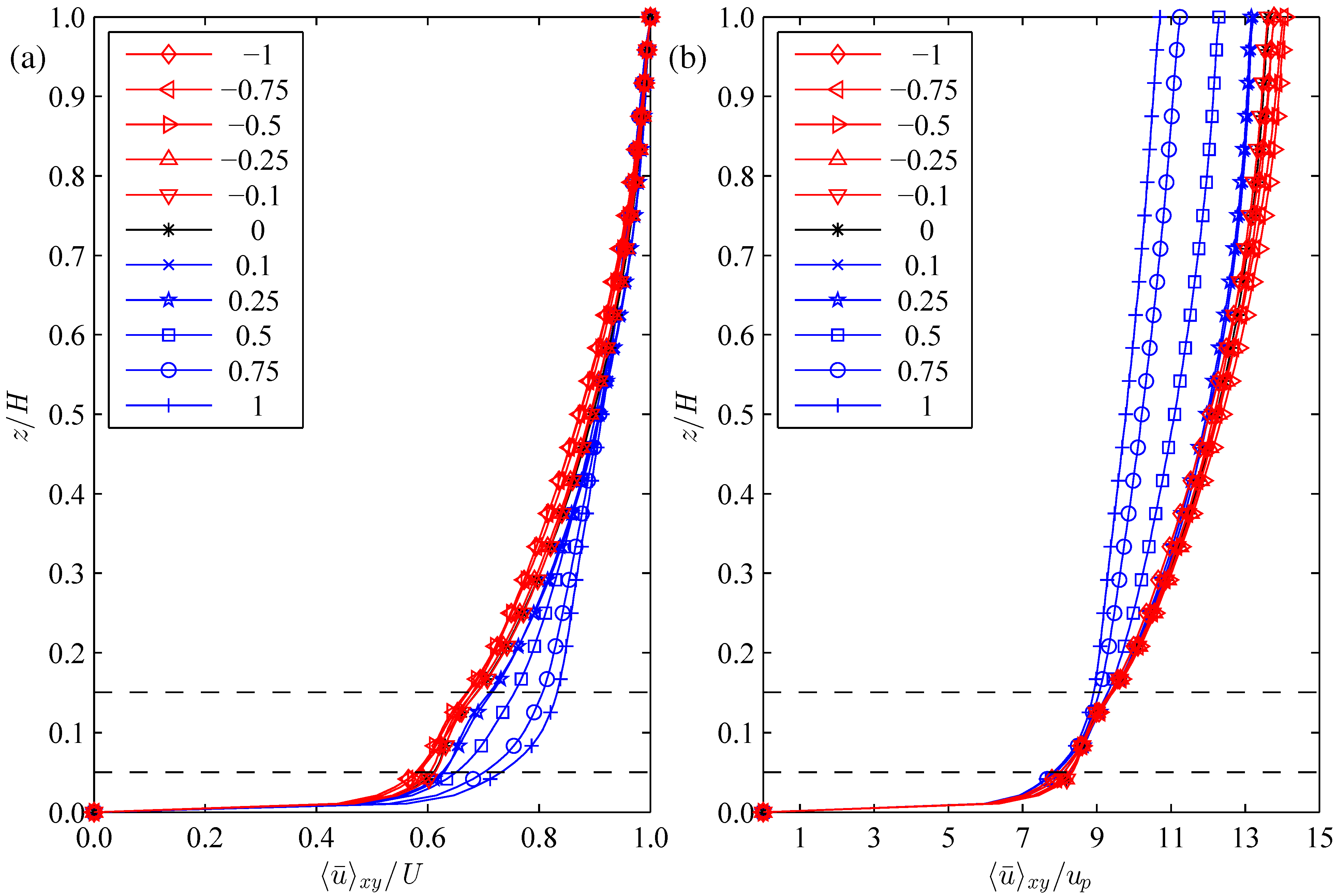
To better understand the increase in wind farm power generation for the A > 0 cases, we now examine the effect of the unconventional forcing scheme on the time-averaged velocity fields. In particular, we focus on the streamwise velocity, which is most directly related to power generation. Figure 4a presents the time-averaged and horizontally-averaged streamwise velocity as a function of the height above ground. Compared to the baseline A = 0 case, the A > 0 forcing scheme blunts the velocity profile, reducing the difference between the high-altitude velocity and the velocity at the turbine hub height. This increase in hub-height velocity correlates with the increase in power extraction shown in Figure 1.

Figure 4. The time-averaged and horizontally-averaged streamwise velocity profiles are shown for all cases (with A given in the legend), normalized by (a) the velocity at the top of the domain and (b) the pressure forcing velocity scale. The turbines rotors are located between the horizontal dashed lines.

Figure 4. The time-averaged and horizontally-averaged streamwise velocity profiles are shown for all cases (with A given in the legend), normalized by (a) the velocity at the top of the domain and (b) the pressure forcing velocity scale. The turbines rotors are located between the horizontal dashed lines.

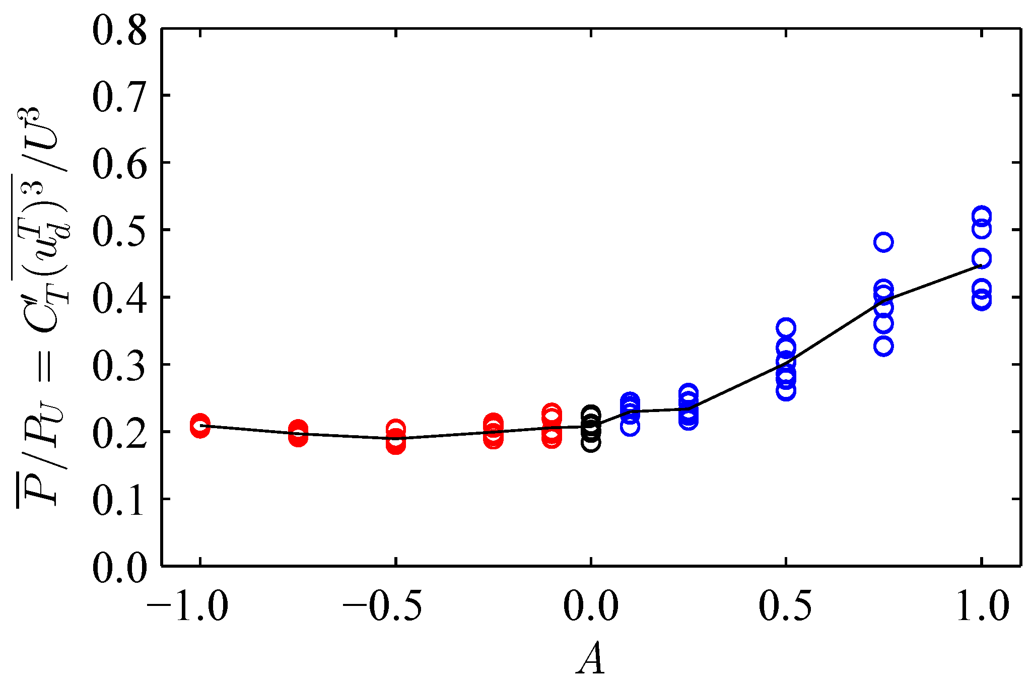
In Section 2.1, we discuss the presentation of the results in terms of the high-altitude velocity U , rather than the pressure-forcing velocity scale u_p. The relationship between these two velocity scales, for each of the forcing cases, is presented in Figure 5. For the A > 0 cases, the pressure-forcing velocityscale is larger compared to the high-altitude velocity, which corresponds to an increase in the height of the boundary layer or the magnitude of the pressure-forcing.

Figure 5. The relationship between the two velocity scales (the pressure-forcing velocity up and the high-altitude velocity U ) is shown for each forcing case. Cases that correlated high-speed flow with upward and downward forcing are colored in red and blue, respectively.

Figure 5. The relationship between the two velocity scales (the pressure-forcing velocity up and the high-altitude velocity U ) is shown for each forcing case. Cases that correlated high-speed flow with upward and downward forcing are colored in red and blue, respectively.

As can be seen in Figure 4b, the average velocity at hub-height (z/H = 0.1), measured in units of the pressure-forcing velocity scale, is independent of the forcing parameter A. The maximum variation in $\overline{u_{\mathrm{d}}^T}$/u_p between cases is found to be 2%, small enough that the predetermined fixed threshold of $\overline{u_{\mathrm{d}}^T}$ = 7.2 in Equation (5) is verified as an appropriate selection. The use of this fixed threshold is additionally desirable, as it uncouples the forcing condition from the flow, thus avoiding one possibility of oscillatory behavior that could arise.

Spatial variation of the streamwise and vertical velocities in the wind farm can be seen in Figure 6 and Figure 7. The length of the time averaging is approximately 1500 tU/H. Figure 6 shows a birds-eye view of the hub-height velocity field for cases A = −1 and A = 1, and Figure 7 shows xz-planes that bisect the wake for A = ±1 and A = 0. The flow has been averaged across all turbine columns for Figure 7 to account for the presence of the high- and low-speed streaks that are clearly visible in Figure 6b. The long time scales of meandering in these high- and low-speed streaks explains the long-time variations in power discussed in Section 3.1. The variability within the wind farm and within the atmospheric flow more generally can be of concern to wind farm operators, so the presence of these streaks could be considered a downside of the forcing scheme.

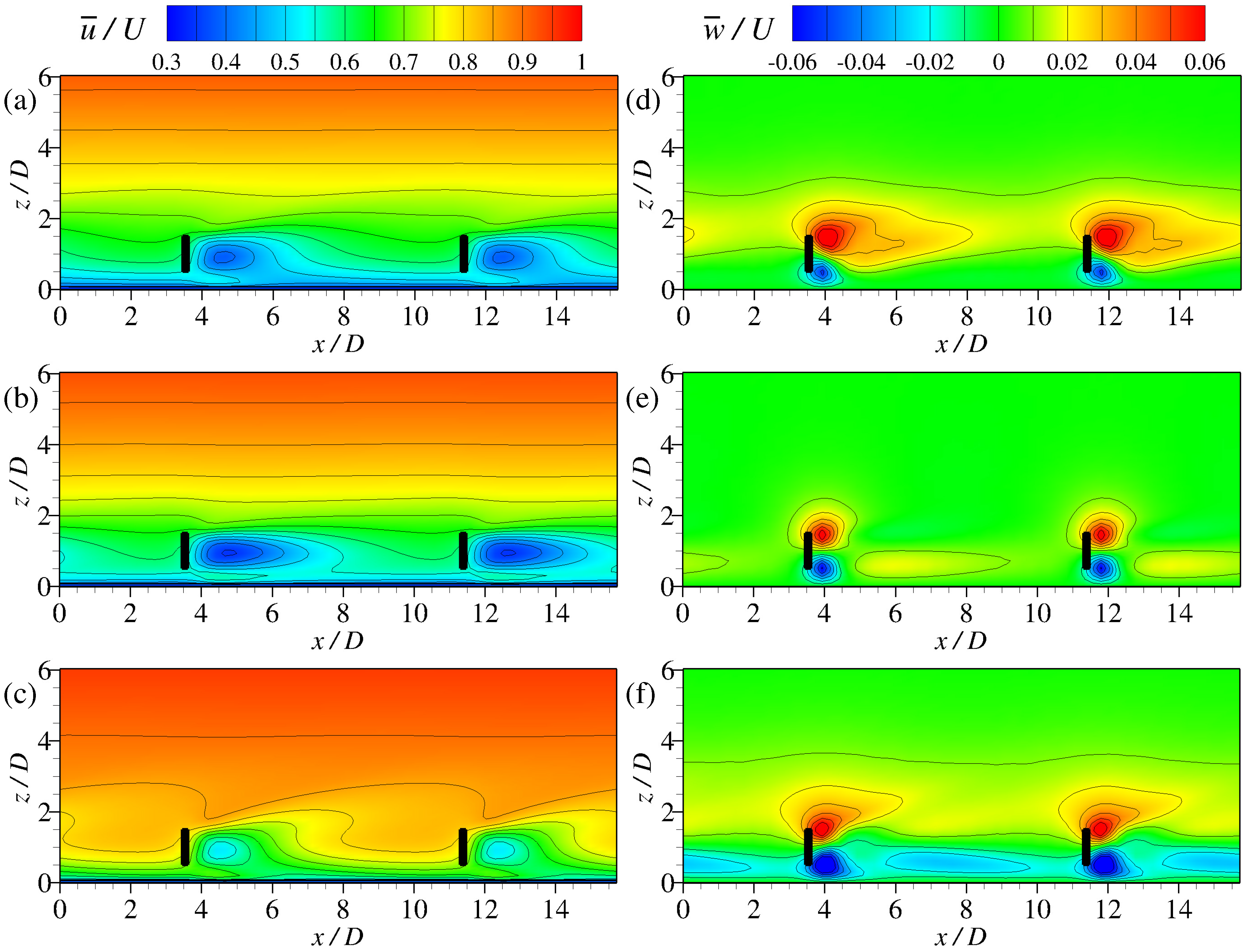
The effect of the forcing scheme on the mean velocity profiles is also visible in the wake bisections shown in Figure 7. Even though the A = −1 case does not have much effect on the power, the wake is clearly altered by the forcing scheme; the A = −1 turbine wake does not extend as far downstream as the baseline A = 0 case (see Figure 7a,b, respectively), but the vertical velocity in the top half of the wake has increased (see Figure 7d compared to Figure 7e). The A = 1 forcing case in Figure 7f shows an increase in the downward velocity within the turbine wake compared to the baseline case in Figure 7e. Importantly, the wake shown in Figure 7c is nearly fully recovered by the next row of turbines, leading to the observed increase in power extraction by the turbines.

Figure 6. Contours of time-averaged streamwise velocity are shown in a horizontal plane at turbine hub height for (a) A = −1 and (b) A = 1. The location of the turbine rotors is indicated by black rectangles.

Figure 6. Contours of time-averaged streamwise velocity are shown in a horizontal plane at turbine hub height for (a) A = −1 and (b) A = 1. The location of the turbine rotors is indicated by black rectangles.

Figure 7. Contours of (a–c) time-averaged streamwise velocity and (d–f) time-averaged vertical velocity are shown on an xz-plane that bisects one column of turbines for: (a,d) A = −1; (b,e) A = 0; and (c,f) A = 1. Only two of the four turbines in the column are shown for each case. The direction of flow is from left to right.

Figure 7. Contours of (a–c) time-averaged streamwise velocity and (d–f) time-averaged vertical velocity are shown on an xz-plane that bisects one column of turbines for: (a,d) A = −1; (b,e) A = 0; and (c,f) A = 1. Only two of the four turbines in the column are shown for each case. The direction of flow is from left to right.

3.3. Mean Kinetic Energy Balance

The power produced by the wind farm, on average, is a function of the MKE $\overline{E}=\frac{1}{2}{\overline{u}}_i{\overline{u}}_i$ at the turbine hub height; in order to increase the wind farm power generation, the MKE at the turbine rotors must increase. The spatial variation of the MKE within the wind farm is shown in Figure 8 for the baseline A = 0 forcing case. The reduction in MKE in the turbine wakes corresponds to energy extraction at the actuator disks. The MKE also increases with the distance from the ground.

Figure 8. Contours of mean kinetic energy (MKE) $\overline{E}=\frac{1}{2}{\overline{u}}_i{\overline{u}}_i$, normalized by the kinetic energy at high altitudes EU = $\frac{1}{2}$U², are shown on three perpendicular planes (x = L, y = L, and z = z_h = D) for the A = 0 baseline case. The turbine rotors are represented by small grey ellipsoids that intersect the z = z_h plane.

Figure 8. Contours of mean kinetic energy (MKE) $\overline{E}=\frac{1}{2}{\overline{u}}_i{\overline{u}}_i$, normalized by the kinetic energy at high altitudes EU = $\frac{1}{2}$U², are shown on three perpendicular planes (x = L, y = L, and z = z_h = D) for the A = 0 baseline case. The turbine rotors are represented by small grey ellipsoids that intersect the z = z_h plane.

To examine the mechanisms by which the MKE varies in space, we consider the transport equation given by:

$$\underset{=0}{\underbrace{{\partial }_{\mathrm{t}}\left(\frac{1}{2}{\overline{u}}_i{\overline{u}}_i\right)}}=\underset{\text{advection}}{\underbrace{-{\overline{u}}_j{\partial }_j\left(\frac{1}{2}{\overline{u}}_i{\overline{u}}_i\right)}}+\underset{\begin{array}{l}\text{wind turbine}\\ \text{power}\end{array}}{\underbrace{{\overline{u}}_i{\overline{f}}_i}}\underset{\begin{array}{l}\text{turbulent}\\ \text{MKE flux}\end{array}}{\underbrace{-{\partial }_j\left[{\overline{u}}_i\left(\overline{u_i^{\prime }{u}_j^{\prime }}+\overline{{\tau }_{ij}^d}\right)\right]}}+\underset{\begin{array}{l}\text{turbulent}\\ \text{MKE dissipation}\end{array}}{\underbrace{\left(\overline{u_i^{\prime }{u}_j^{\prime }}+\overline{{\tau }_{ij}^d}\right){\partial }_j{\overline{u}}_i}}\underset{\text{pressure power}}{\underbrace{-\frac{1}{\mathrm{\rho }}{\partial }_i\left[{\overline{u}}_i\widehat{p}+{\delta }_{i1}{\overline{u}}_i{p}_{\infty }\right]}}$$

(6)

with $\widehat{p}$ = p+1/3ρτ_kk. The MKE is transported by advection and turbulent kinetic energy flux, decreased by wind turbine power extraction and turbulent dissipation and increased by pressure power from the driving pressure gradient. The magnitude of each of these terms, averaged over horizontal planes, is shown for A = ±1 and A = 0 in Figure 9. For every case, the primary balance is between the power extraction by the wind turbines and the MKE turbulent flux.

Figure 9. Horizontally-averaged terms in the MKE balance are shown as a function of height for three forcing cases: (a) A = −1; (b) A = 0; and (c) A = 1. Each symbol represents the horizontal average of a single term in Equation (6): advection (★); MKE flux (•); MKE dissipation (■); and turbine power extraction (▼). The turbine rotors are located in the region between the dashed lines.

Figure 9. Horizontally-averaged terms in the MKE balance are shown as a function of height for three forcing cases: (a) A = −1; (b) A = 0; and (c) A = 1. Each symbol represents the horizontal average of a single term in Equation (6): advection (★); MKE flux (•); MKE dissipation (■); and turbine power extraction (▼). The turbine rotors are located in the region between the dashed lines.

Since we are primarily interested in increasing the MKE at the height of the turbine rotors, we average Equation (6) over the volume defined by z_h− D/2 ≤ z ≤ z_h + D/2 (the vertical range of the turbine rotors) and all x and y to obtain:

$$0=𝒜+{𝒫}_{\tau }+\Phi +𝒟+ℛ$$

(7)

with advection 𝒜, wind turbine power $𝒫$_τ, MKE flux $\Phi$, MKE dissipation $𝒟$ and the remainder $ℛ$ defined as follows:

$$𝒜={\displaystyle \underset{0}{\overset{L}{\int }}{\displaystyle \underset{0}{\overset{L}{\int }}{\displaystyle \underset{z_{\mathrm{h}}-D/2}{\overset{z_{\mathrm{h}}+D/2}{\int }}-{\overline{u}}_j{\partial }_j\text{(}\frac{1}{2}{\overline{u}}_i{\overline{u}}_i)\mathrm{d}{x}_3\mathrm{d}{x}_2\mathrm{d}{x}_1}}}\text{=}{\displaystyle \underset{0}{\overset{L}{\int }}{\displaystyle \underset{0}{\overset{L}{\int }}-\frac{1}{2}{\overline{u}}_3{\overline{u}}_i{\overline{u}}_i{|}_{(z_{\mathrm{h}}-D/2)}^{(z_{\mathrm{h}}+D/2)}\mathrm{d}{x}_2\mathrm{d}{x}_1}}$$

(8)

$${𝒫}_{\tau }={\displaystyle \underset{0}{\overset{L}{\int }}{\displaystyle \underset{0}{\overset{L}{\int }}{\displaystyle \underset{z_{\mathrm{h}}-D/2L}{\overset{z_{\mathrm{h}}+D/2}{\int }}{\overline{u}}_i{\overline{f}}_i\mathrm{d}{x}_3\mathrm{d}{x}_2\mathrm{d}{x}_1}}}$$

(9)

$$\mathrm{\Phi }={\displaystyle \underset{0}{\overset{L}{\int }}{\displaystyle \underset{0}{\overset{L}{\int }}{\displaystyle \underset{z_{\mathrm{h}}-D/2}{\overset{z_{\mathrm{h}}+D/2}{\int }}-{\partial }_j[{\overline{u}}_i(\overline{u_i^{\prime }{u}_j^{\prime }}+\overline{{\tau }_{ij}^d})]\mathrm{d}{x}_3\mathrm{d}{x}_2\mathrm{d}{x}_1}}}={\displaystyle \underset{0}{\overset{L}{\int }}{\displaystyle \underset{0}{\overset{L}{\int }}-{\overline{u}}_i(\overline{{u^{\prime }}_i{u^{\prime }}_3}+\overline{{\tau }_{i3}^d}){|}_{(z_{\mathrm{h}}-D/2)}^{(z_{\mathrm{h}}+D/2)}\mathrm{d}{x}_2\mathrm{d}{x}_1}}$$

(10)

$$𝒟={\displaystyle \underset{0}{\overset{L}{\int }}{\displaystyle \underset{0}{\overset{L}{\int }}{\displaystyle \underset{z_{\mathrm{h}}-D/2}{\overset{z_{\mathrm{h}}h+D/2}{\int }}\left(\overline{{u^{\prime }}_i{u^{\prime }}_j}+\overline{{\tau }_{ij}^d}\right){\partial }_j{\overline{u}}_i\mathrm{d}d{x}_3\mathrm{d}{x}_2\mathrm{d}{x}_1}}}$$

(11)

$$ℛ=-𝒜-P_{\tau }-\mathrm{\Phi }-D$$

(12)

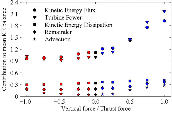
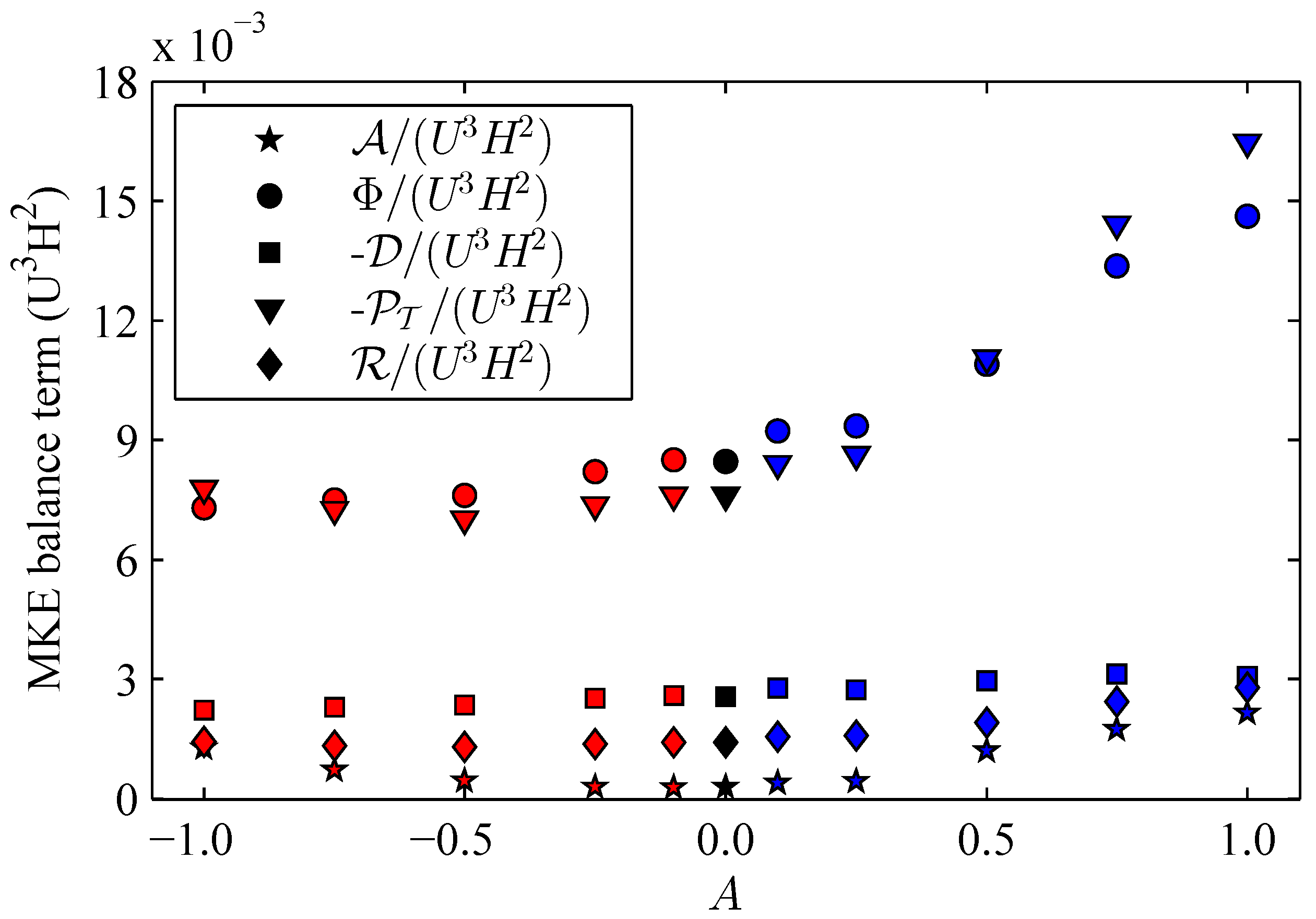
The contribution from each term is shown in Figure 10 as a function of the forcing parameter A.

Figure 10. The contribution of MKE in the turbine region due to each term in the MKE balance (Equations (8)–(11)) is shown as a function of the forcing parameter A.

Figure 10. The contribution of MKE in the turbine region due to each term in the MKE balance (Equations (8)–(11)) is shown as a function of the forcing parameter A.

Consistent with previous findings [17,18,19,20,21], the increase in power produced by the wind farm correlates with an increase in turbulent MKE flux; these two terms continue to dominate the MKE balance in the presence of the unconventional forcing scheme. Somewhat surprisingly, the MKE dissipation is only slightly affected by the vertical forcing despite the strong increase in mixing within the boundary layer. The slightly larger power output at turbines compared to the integrated MKE flux for A > 0.5 can be attributed to the increase in the advection and the energy input from the pressure-forcing contained within the remainder term.

4. Conclusions

Based on the results of this study, it appears that synthetic vertical forcing at the turbines can have a significant effect on the power extraction and the MKE entrainment in a large wind turbine array. When downward forcing corresponds with high velocities, the vertical mixing is increased, leading to more blunt velocity profiles and, thus, to higher velocities at the turbine disk for a given high-altitude velocity. This increase leads to an improvement of turbine power and kinetic energy flux to the turbines. The vertical forcing also has an effect on the spatial distribution of streamwise velocity within the wind farm, leading to the more pronounced formation of high- and low-speed streaks, which may be relevant to wind farm operation and control schemes. Interestingly, the scheme in which upward forcing corresponds to high velocity has little effect on the performance of the wind farm.

These results were obtained for a simplified setup that ignored several physical processes that could be important, such as Coriolis-induced rotation of the wind vector with height, thermal stratification effects and angular momentum in turbine wakes. Now that coarse simulation results have suggested that forcing can positively affect entrainment and power extraction, additional physical processes can be incorporated in more finely-resolved simulations that should be performed as a next step.

The vertical forces imposed for the extreme cases in this study would likely be impractical or impossible to implement in practice. The most extreme case, however, improves power extraction by as much as 95%; even a much smaller increase in power production, say 5%, from a more moderate and realistic forcing scheme would be worth investigating. At this stage, no attempt is made to compare the net energy gain with the energy that would be required to impose this active forcing. Since only a small subset of possible forcing schemes are examined in this study, it appears possible that practically realizable and effective active forcing schemes could be developed.