Numerical Validation of a Vortex Model against ExperimentalData on a Straight-Bladed Vertical Axis Wind Turbine

Abstract

Cyclic blade motion during operation of vertical axis wind turbines (VAWTs) imposes challenges on the simulations models of the aerodynamics of VAWTs. A two-dimensional vortex model is validated against the new experimental data on a 12-kW straight-bladed VAWT, which is operated at an open site. The results on the normal force on one blade are analyzed. The model is assessed against the measured data in the wide range of tip speed ratios: from 1.8 to 4.6. The predicted results within one revolution have a similar shape and magnitude as the measured data, though the model does not reproduce every detail of the experimental data. The present model can be used when dimensioning the turbine for maximum loads.

1. Introduction

The interest in vertical axis wind turbines (VAWTs) as an alternative to the conventional horizontal axis wind turbines (HAWTs) has been growing in recent years [1]. This is due to the potential of VAWTs to decrease the cost of wind energy [2,3]. VAWTs have several advantages over HAWTs: the generator of a VAWT can be located at the ground level, therefore excluding the concerns over the mass and size of the generator. The advantage of the lower center of mass (compared to HAWTs) is very important for floating platforms [4]. Additionally, the yawing mechanism is excluded for VAWTs, since they are omni-directional. Thus, the simplicity of the concept with only a few moving parts is one of the main advantages of VAWTs over HAWTs.

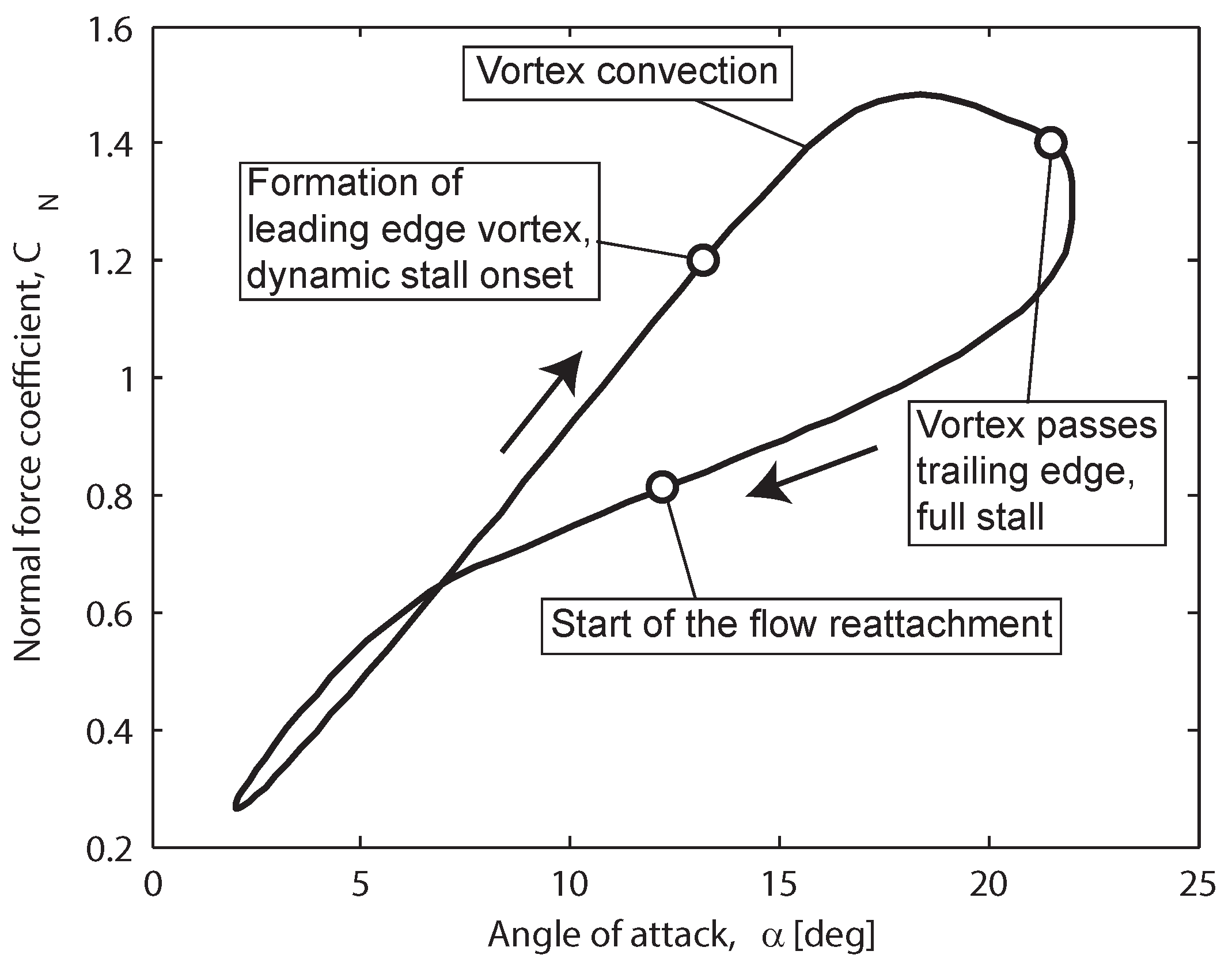
The complex aerodynamics of VAWTs imposes significant challenges on the simulation models. The flow velocity at the blades of the VAWT changes constantly during the turbine rotation, which causes the angle of attack to change during every revolution. The magnitude of the variation of the angle of attack increases with the decreased turbine tip speed ratio (TSR). At low TSRs, the blades of the VAWT experience the event of dynamic stall, which is associated with the rapid decrease in the lift and the increase in the drag force, reducing the torque on the turbine. At high TSRs, the flow velocity when passing through the turbine is decreased more than at low TSRs, and therefore, the flow expansion is prevailing at high TSRs.

The simulation models for VAWTs can be divided into three groups. The first group includes the finite element method (FEM) or the finite volume method (FVM), which are used to solve the Navier–Stokes equations within the commonly-available software for computational fluid dynamics (CFD). The second method is based on the vorticity equation, and the models are usually referred to as vortex models. The third method is based on the momentum conservation principle, and one of the most common and advanced momentum models is the double multiple streamtube model. The overview of the aerodynamic models for VAWTs can be found in [5,6,7]. A two-dimensional (2D) vortex model combined with the Leishman–Beddoes-type dynamic stall model is used in this study. The model combines the vorticity equation with experimental data, which results in the high computational speed of the model. This model gives the flow velocity field and is time dependent.

There is a lack of experimental data on the blade forces during one revolution for VAWTs. A series of the experiments were conducted by the Sandia National Laboratories in the 1980s, where VAWTs with curved blades (Darrieus turbines) were operated at open sites [8,9,10]. Other measured data concern small vertical axis turbines operating in wind tunnels or towing tanks with low operational Reynolds numbers [11,12]. Since the force coefficients are dependent on the Reynolds number, the aerodynamics of large turbines are different from the aerodynamics of turbines operated in wind tunnels or towing tanks. Thus, due to high Reynolds numbers, the measured data from the Sandia National Laboratories are still used for the validation of simulation models [13,14,15,16].

This study assesses measurements from 2014 on a straight-bladed VAWT, which operates at an open site with the average Reynolds number of $300,000$ [17,18]. A study on the power coefficient ($C_P$) of this VAWT from 2011 has shown that the turbine reaches its maximum $C_P$ of 0.29 at the TSR of 3.3 [19]. However, the turbine diameter has increased from 6 to 6.5 m after mounting the load cell assembly, and the power coefficient is expected to be slightly different for the modified turbine as the turbine solidity has decreased. New experimental data on the normal forces on this VAWT are presented. The goal of the study is to describe the simulation model and to validate it against the experimental data. The normal forces are compared for the range of TSRs from 1.8 to 4.6, covering the dynamic stall region and the region of high flow expansion. The results and the capability of the model are analyzed.

2. Experimental Data

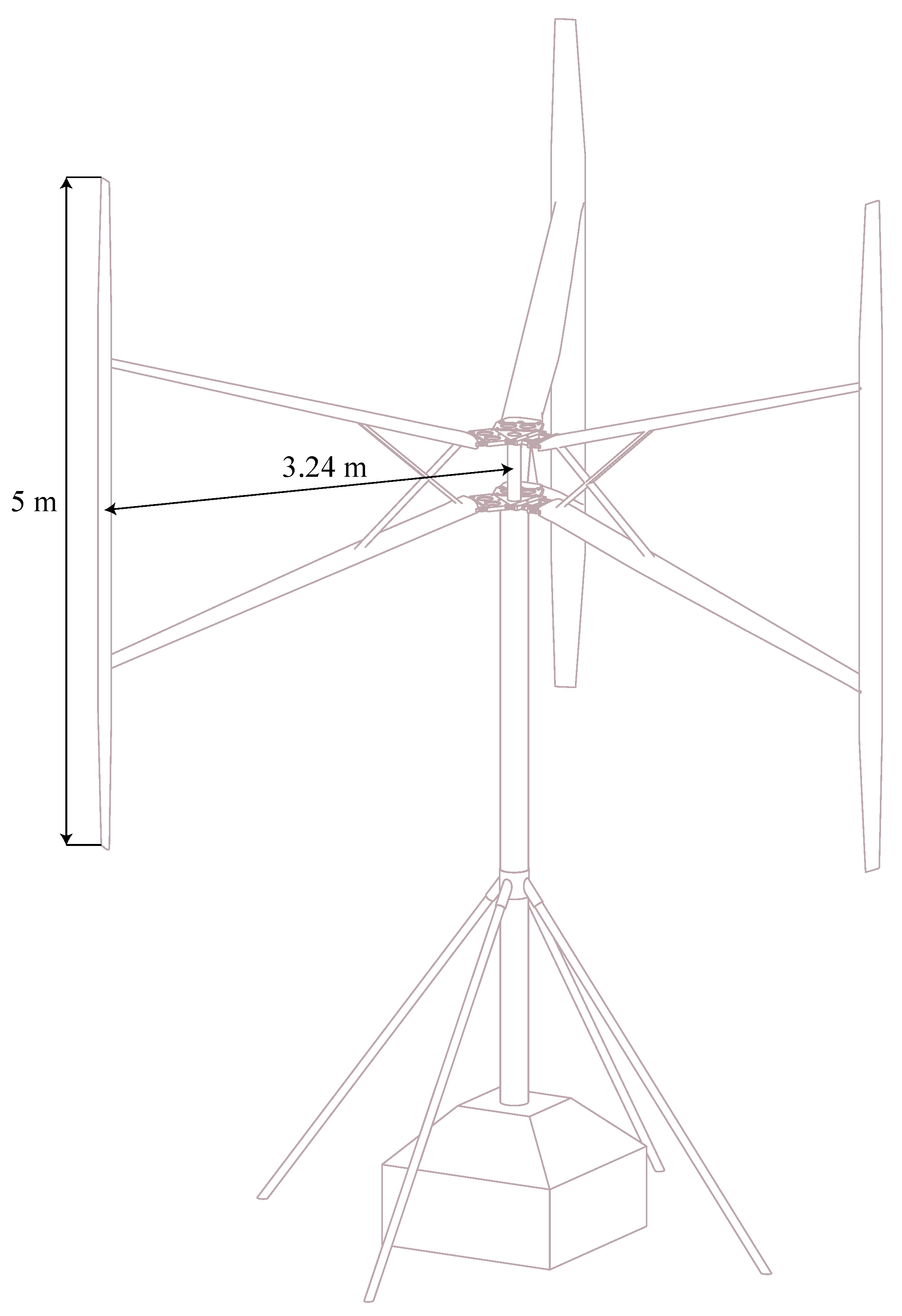
The measurement data used in this study are obtained from the 12-kW VAWT located outside Uppsala, Sweden. The experimental method and the obtained force data are described in detail in [17,18]. It follows that the measured normal force was periodic and consistent, while the tangential force response was highly disturbed by the turbine dynamics. Hence, only the normal force measurements can be considered suitable for usage in this validation. 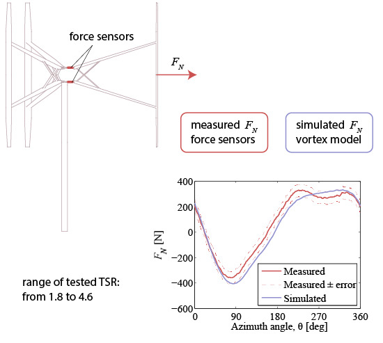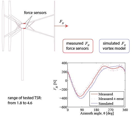The studied VAWT is a 3-bladed H-rotor turbine with a radius of 3.24 m and a blade length of 5 m; Figure 1. The blades are pitched outwards 2 degand have the NACA0021profile with a chord length of 0.25 m at the middle of the blade. 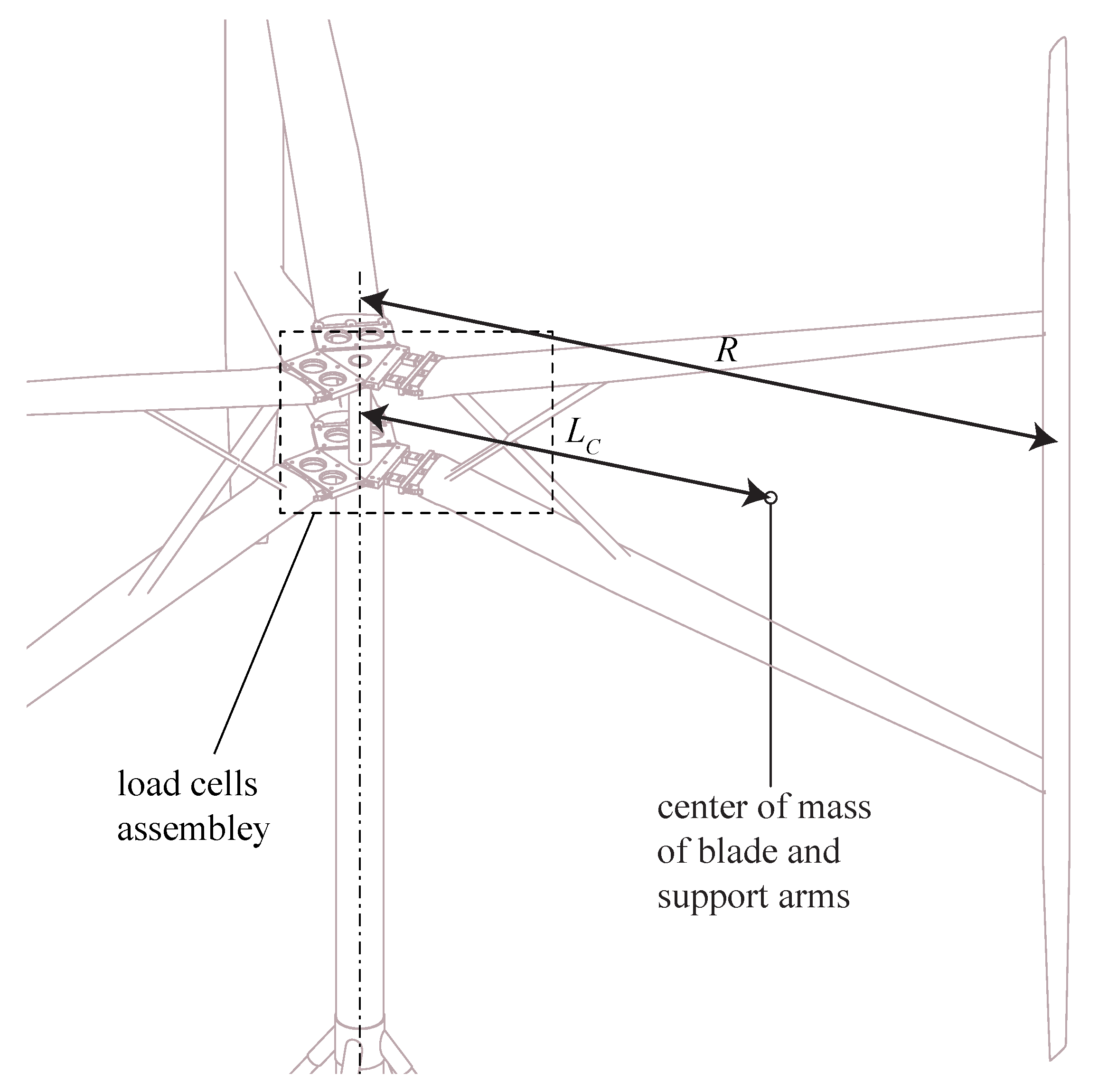The turbine with assembled force sensors is shown in Figure 2 and Figure 3. The sensors are single-axis load cells, which measure tension and compression at a point load. The rotational speed of this turbine can be kept at a constant level [17,19], and the normal force is estimated using the notations from Figure 2 and Figure 3 as the following:

$$F_N=F_0+F_1+F_2+F_3-F_C$$

(1)

where $F_C$ is the centrifugal force:

$$F_C=m{\Omega }^2{L}_C$$

(2)

Figure 1. The vertical axis wind turbine (VAWT) used for the experiment.

Figure 1. The vertical axis wind turbine (VAWT) used for the experiment.

Figure 2. Load cells installed on the VAWT.

Figure 2. Load cells installed on the VAWT.

Figure 3. The assembly of the load cells. The notation of the measured forces.

Figure 3. The assembly of the load cells. The notation of the measured forces.

Here, $m=35.79\mathrm{kg}$ is the mass of the blade and support arms, Ω is the turbine rotational speed and $L_C=1.83\mathrm{m}$ is the distance from the axis of rotation to the center of mass of the blade assembled with the support arms. $F_0$, $F_1$, $F_2$ and $F_3$ are the measured forces.

Due to varying weather conditions, the force measurements were analyzed only for times with steady wind flow conditions. The relative standard deviation (RSD) was used to quantify wind flow variations:

$$RSD\left(x\right)={\left(\frac{1}{n}\sum _{j=1}^n{\left(x_j-\langle x\rangle \right)}^2\right)}^{\frac{1}{2}}\frac{1}{\langle x\rangle }\times 100\%$$

(3)

where $\langle x\rangle$ denotes the average value of variable x.

The measured data were divided into 24 s-long bins: 16 s to stabilize the turbine wake (“wake time”, corresponding to 10 revolutions at 40 rpm) followed by 8 s of steady flow operation (“disk time”, 5 revolutions at 40 rpm). Wind flow was considered as steady for bins with the RSD of the asymptotic wind velocity $V_{\infty }$ of $RS{D}_{wake}\left(V_{\infty }\right)\le 10\%$, $RS{D}_{disk}\left(V_{\infty }\right)\le 5\%$ and the RSD of wind direction $Vdir$ of $RS{D}_{wake,disk}\left(Vdir\right)\le 1\%$. This definition of the steady wind flow conditions is documented in [18]. Variations of the wind speed during the steady conditions are illustrated in Figure 4.

Figure 4. Allowed variations of the asymptotic wind velocity inside a bin with the steady wind flow conditions.

Figure 4. Allowed variations of the asymptotic wind velocity inside a bin with the steady wind flow conditions.

The normal force during one revolution is obtained as the average response over 5 revolutions with steady wind flow. The operational TSR is estimated as:

$$\lambda =\frac{〈\Omega 〉R}{〈V_{\infty }〉}$$

(4)

where Ω is the turbine rotational speed. The average values of Ω and $V_{\infty }$ are taken taken over time with steady wind flow.

The analysis of the measurement accuracy has shown that the maximum error of the measured normal force is a function of the turbine rotational speed:

$$\Delta F_N=\pm \left(0.0049{\Omega }_{\mathrm{rpm}}^2+0.072{\Omega }_{\mathrm{rpm}}+23\right)$$

(5)

where ${\Omega }_{\mathrm{rpm}}$ is the rotational speed in $\mathrm{rpm}$. For the details regarding the measurement accuracy, the reader is referred to [17,18]. The air density ρ is calculated for the measured air temperature, pressure and humidity according to [17]. The kinematic viscosity ν is estimated as the function of the measured air temperature [20].

3. Simulation Model

This section presents the vortex method together with the dynamic stall model to predict the blade forces of the VAWT. The sign notation of the forces together with the blade azimuth angle are defined in Figure 5.

Figure 5. The sign convention of the normal and tangential forces. The counter-clockwise direction of the blade azimuth angle θ is defined as positive.

Figure 5. The sign convention of the normal and tangential forces. The counter-clockwise direction of the blade azimuth angle θ is defined as positive.

3.1. Vortex Model of the Turbine

The vortex method is commonly used for solving the flow of vertical axis turbines. The main idea behind the model is to use the vorticity as the discretization variable, instead of the velocity. The vorticity is obtained by taking the curl of the flow velocity:

$$\overrightarrow{\omega }=\nabla \times \overrightarrow{V}$$

(6)

and similarly, the vorticity equation is obtained from the curl of the Navier–Stokes equations:

$$\frac{\partial \overrightarrow{\omega }}{\partial t}+\left(\overrightarrow{V}·\nabla \right)\overrightarrow{\omega }=\left(\overrightarrow{\omega }·\nabla \right)\overrightarrow{V}+\nu {\nabla }^2\overrightarrow{\omega }$$

(7)

which in the two-dimensional case becomes:

$$\frac{\partial \overrightarrow{\omega }}{\partial t}+\left(\overrightarrow{V}·\nabla \right)\overrightarrow{\omega }=\nu {\nabla }^2\overrightarrow{\omega }$$

(8)

The current implementation uses a free vortex model, where the individual vortices are used as discretization variables. The flow velocity is obtained from the model as a superposition of the potential flow solution and the contribution from the vortices:

$$\overrightarrow{V}=\nabla \varphi +{\overrightarrow{V}}_{\omega }$$

(9)

Under the assumption that the turbine is not confined with walls and that that the blade is approximated as a single point, the potential flow solution $\nabla \varphi$ is equal to the asymptotic flow velocity $V_{\infty }$. For the two-dimensional vortex method, according to the Biot–Savart law and using the complex numbers, the velocity contribution from vortices ${\overrightarrow{V}}_{\omega }$ at position r becomes:

$$V_{\omega }\left(r\right)=\sum _{k=1}^{N_{\nu }}\frac{i{\Gamma }_k}{2\pi }\frac{1}{\left(\overline{r}-{\overline{r}}_k\right)}\left(1-e^{-\frac{{\left|\overline{r}-{\overline{r}}_k\right|}^2}{{\epsilon }^2}}\right)$$

(10)

Here, $r_k$ is the position and ${\Gamma }_k$ is the circulation of vortex k (${\overline{r}}_k$ denotes the complex conjugate of $r_k$); $N_v$ is the total number of released vortices. The Gaussian kernel $\left(1-e^{-\frac{{\left|r-r_k\right|}^2}{{\epsilon }^2}}\right)$ is used to avoid the non-physical divergences when r approaches $r_k$ [21].

The relative wind velocity at the turbine blades is a vector sum of the flow velocity at the blade due to its own motion, $-{\overrightarrow{V}}_b$ and the flow velocity $\overrightarrow{V}$:

$${\overrightarrow{V}}_{rel}=\overrightarrow{V}-{\overrightarrow{V}}_b$$

(11)

where the velocity $\overrightarrow{V}$ is given by Equations (9) and (10), and the blade tangential velocity ${\overrightarrow{V}}_b$ is:

$${\overrightarrow{V}}_b=\Omega R\widehat{t}$$

(12)

Here, $\widehat{t}$ is the unit vector in the tangential direction with the same sign convention as the blade azimuth angle θ in Figure 5. In the Lagrangian formulation, the vortices are allowed to drift with the flow velocity. Neglecting the viscosity outside the boundary layers of the blades, the vortices are propagated according to:

$$\frac{d\overrightarrow{r}}{dt}=\overrightarrow{V}\left(\overrightarrow{r}\right)$$

(13)

where the velocity $\overrightarrow{V}$ is calculated with Equations (9) and (10). The velocities at each vortex position can efficiently be evaluated using the fast multipole method [22], and the current work uses the implementation described in [23].

Even though the vortex method can solve the entire flow, a full solution of the boundary layer will require a high computational effort. To significantly improve the speed, a dynamic stall model of the blade force coefficients is used to obtain the lift and drag coefficients; see Section 3.2. The dynamic stall model requires the flow velocity and the angle of attack to be calculated. The absolute value of the relative flow velocity $V_{rel}=|{\overrightarrow{V}}_{rel}|$ is calculated with Equations (9) to (11) and is used as an input to the blade force model. To properly handle the flow curvature effects from the rotating motion of the turbine, the blade geometry has to be modeled. In the current implementation, the blade is modeled with linear panels with the linear distribution of vorticity according to [5,24]. Using these panels, the bound circulation of the blades ${\Gamma }_{blade}$ can be determined by enforcing the no-penetration boundary condition on the surface of airfoil and the Kutta condition on the trailing edge. This circulation can be used to calculate the corresponding angle of attack:

$$\alpha =p\left(arcsin\left(\frac{{\Gamma }_{blade}}{\pi c{V}_{rel}}\right)-{\alpha }_0\right)$$

(14)

where c is the blade chord length and parameters p and ${\alpha }_0$ are determined by matching the bound circulation ${\Gamma }_{blade}$ with the known angle of attack from the steady-state potential flow solutions. The procedure of calculating the angle of attack is described in greater detail in [25], and the method denoted “explicit method” is the one implemented here. This method adds the released vortex into the panel equations and solves for the Kutta condition together with the conservation of circulation, i.e., the total circulation of the released vortex, and the bound circulation should equal the bound circulation from the previous time step.

With the velocity $V_{rel}$, the angle of attack α and its time derivative $\dot{\alpha }$, the lift and the drag force coefficients ($C_L$ and $C_D$) are obtained within the blade force model for an airfoil profile with a given chord length c and the Reynolds number (Section 3.2, Equation (31)). Please note that only symmetrical four-digit NACA airfoils are implemented in this work. The kinematic viscosity, obtained from the weather data (Section 2), is used in the model to estimate the local Reynolds number. The lift force coefficient from the blade force model can then be used to calculate the effective bound circulation ${\Gamma }_{ds}$ with the Kutta–Joukowski lift formula:

$${\Gamma }_{ds}=\frac{1}{2}{C}_{L}c{V}_{rel}$$

(15)

Due to conservation of circulation, a vortex has to be released from the trailing edge of the blade each time step $\Delta t$ with a strength ${\Gamma }_{released}$ corresponding to the change of circulation between the time steps:

$${\Gamma }_{released}={\Gamma }_{ds,n-1}-{\Gamma }_{ds,n}$$

(16)

where subscripts n and $n-1$ stand for current and previous time steps. The position of the released vortex is chosen as $0.5\Omega R\Delta t$ behind the trailing edge. In the case of dynamic stall, the bound circulation of the blade will be reduced, i.e., ${\Gamma }_{ds}<{\Gamma }_{blade}$. This means that the blade will no longer fulfil the Kutta condition, which then would give infinite flow velocities at the trailing edge. Therefore, during the evaluation of the vortex velocities, it is chosen to approximate the blade as a single point vortex (located at a quarter-chord position) that can be evaluated with Equation (10). This approximation also increases the computational speed (compared to modeling the blades with panels) as no panel to vortex interactions have to be calculated. This approximation is evaluated in [25], and the results show that the difference between approximating the blade with a point vortex or with panels is very small; hence, the approximation is reasonable.

All simulations were performed for 100 turbine revolutions to ensure convergence in the results. This value was chosen from the convergence studies performed in [26]. One hundred twenty time steps were performed for each revolution, and the turbine was kept at a constant rotational speed for the entire simulation. The normal force was calculated based on the obtained lift and drag coefficients:

$$F_N=\frac{1}{2}\rho A_{blade}{V}_{rel}^2\left(C_{L}cos\phi +C_{D}sin\phi \right)$$

(17)

with blade area $A_{blade}$ and air density ρ. The angle φ is the angle of the relative flow velocity vector ${\overrightarrow{V}}_{rel}$. The force values are presented from the last revolution of the simulations. An overview of the vortex model algorithm is illustrated in Figure 6, where the most important steps are highlighted.

Figure 6. Flow chart of the vortex model combined with the dynamic stall (DS) model. $N_{step}$ is the current time step, and $N_{step,max}$ is the maximum number of time steps. $N_{step,max}=12,000$, corresponding to 120 time steps per each of 100 revolutions.

Figure 6. Flow chart of the vortex model combined with the dynamic stall (DS) model. $N_{step}$ is the current time step, and $N_{step,max}$ is the maximum number of time steps. $N_{step,max}=12,000$, corresponding to 120 time steps per each of 100 revolutions.

3.2. Dynamic Stall Modeling

The model originally developed by Leishman and Beddoes [27,28] with modifications for the conditions of VAWTs [29,30] is used for the modeling of the dynamic stall. The dynamic stall model uses experimental data of the lift and the drag coefficients for steady flow over airfoils [31]. This model was combined with the vortex model for a single pitching wing and showed reasonable agreement with experimental data on the pitching airfoils [25]. The inputs to the models are the angle of attack α and its rate of change $\dot{\alpha }$, the velocity $V_{rel}$, the chord length c, the Reynolds number and the blade airfoil. These inputs are obtained within the vortex model. The outputs of the dynamic stall model are the lift and the drag coefficients ($C_L$ and $C_D$, respectively). The main principles of the model are described in this section, and the reader is referred to [25,29] for the details, including the empirical parameters.

The Leishman–Beddoes dynamic stall model consists of three parts: unsteady attached flow, dynamic stall onset and unsteady separated flow part. The unsteady attached flow solution comprises impulsive and circulatory loading, which are caused by unsteady boundary vortex and the changes in the angles of attack. The change of the flow velocity due to the vortex contribution is already taken into account by the vortex model. Thus, the unsteady attached flow part of the Leishman–Beddoes model is not used when combined with the vortex model. This method is identical to the one described in [25].

A delay in the pressure response is represented by the further lag in the angle of attack:

$${\alpha }_n^{\prime }={\alpha }_n-D_{{\alpha }_n}$$

(18)

where $D_{\alpha }$ is the deficiency function:

$$D_{{\alpha }_n}=D_{{\alpha }_{n-1}}exp\left(-\frac{\Delta s}{T_{\alpha }}\right)+\left({\alpha }_n-{\alpha }_{n-1}\right)exp\left(-\frac{\Delta s}{2T_{\alpha }}\right)$$

(19)

Here, $T_{\alpha }$ is an empirically-derived constant, and its values for the symmetrical NACA-airfoils are found in [29]. For the NACA0021 airfoil, $T_{\alpha }=6.30$. The non-dimensional time step $\Delta s$ is calculated as:

$$\Delta s=\frac{2V_{rel}\Delta t}{c}$$

(20)

where $V_{rel}$ is the relative flow velocity obtained from Equation (11).

A critical angle of attack is defined to represent the onset of the dynamic stall:

$${\alpha }_{c{r}_n}=\left\{\begin{array}{cc}{\alpha }_{ds0}\hfill & \left|q_n\right|\ge q_0\hfill \\ {\alpha }_{ss}+\left({\alpha }_{ds0}-{\alpha }_{ss}\right)\frac{\left|q_n\right|}{q_0}\hfill & \left|q_n\right|<q_0\hfill \end{array}\right.$$

(21)

with the reduced pitch rate q as:

$$q_n=\frac{\dot{{\alpha }_n}c}{2V_{rel}}$$

(22)

Here, $q_0$ is the reduced pitch rate, which delimits the quasi-steady stall and the dynamic stall; $q_0=0.01$. ${\alpha }_{ds0}$ and ${\alpha }_{ss}$ are the critical static stall onset angle and the static stall angle, respectively, ${\alpha }_{ds0}=17.{91}^{°}$ and ${\alpha }_{ss}=14.{33}^{°}$ for NACA0021 [29]. The dynamic stall condition is defined as when the delayed angle of attack ${\alpha }^{\prime }$ exceeds the critical angle of attack ${\alpha }_{cr}$:

$$\left|{\alpha }^{\prime }\right|>{\alpha }_{cr}\to \mathrm{stall}$$

(23)

The unsteady separated flow part includes the trailing edge and the leading edge vortex separation. The trailing edge separation is associated with the delay in the convection of the flow separation point over the surface of the airfoil. It is represented via Kirchhoff’s flow approximation:

$$f_n^{\prime }=\left\{\begin{array}{cc}1-0.4exp\left(\frac{\left|{\alpha }_n^{\prime }\right|-{\alpha }_1}{S_1}\right)\hfill & \left|{\alpha }_n^{\prime }\right|<{\alpha }_1\hfill \\ 0.02+0.58exp\left(\frac{{\alpha }_1-\left|{\alpha }_i^{\prime }\right|}{S_2}\right)\hfill & \left|{\alpha }_n^{\prime }\right|\ge {\alpha }_1\hfill \end{array}\right.$$

(24)

where $f^{\prime }$ is the delayed separation point and $S_1$, $S_2$ and ${\alpha }_1$ are the empirically-derived constants, which are based on the local Reynolds number and the airfoil profile and are found in [29]. In addition to the pressure response delay (which is represented by ${\alpha }^{\prime }$, Equation (18)), a further delay in the flow separation point is present in order to account for the time-dependent boundary layer:

$$f_i^{″}=f_i^{\prime }-D_{f_i}$$

(25)

where $D_{f_n}$ is:

$$D_{f_n}=D_{f_{n-1}}exp\left(-\frac{\Delta s}{T_f}\right)+\left(f_n^{\prime }-f_{n-1}^{\prime }\right)exp\left(-\frac{\Delta s}{2T_f}\right)$$

(26)

Here, $T_f=3$, which is the empirically-derived constant [29]. The normal force coefficient for the unsteady separated flow conditions before the dynamic stall onset is:

$$C_{N_n}^f=C_{N_{\alpha }}{\alpha }_n{\left(\frac{1+\sqrt{f_n^{″}}}{2}\right)}^2$$

(27)

where $C_{N_{\alpha }}$ is the slope of the normal force coefficient at the static conditions, and it is based on the airfoil and the Reynolds number [29].

When the dynamic stall condition is met (Equation (23)), the leading edge vortex forms and propagates towards the trailing edge and then releases. This vortex convection is represented by an increase in the lift force (sometimes referred to as the vortex lift) during the vortex propagation and followed by a drop in the lift force when the vortex releases. The vortex lift is calculated as the follows:

$$C_{N_n}^v=B_1\left(f_n^{″}-f_n\right)V_x$$

(28)

where f is the static separation point and $B_1$ and $V_x$ are parameters, which are based on the local Reynolds number and the blade airfoil and are found in [29].

The total normal force coefficient is the sum of the unsteady normal force coefficient and the vortex lift:

$$C_{N_n}=C_{N_n}^f+C_{N_n}^v$$

(29)

An example of the force response during the pitching motion of an airfoil is shown in Figure 7, and the features mentioned above are noted. The tangential force coefficient $C_T$ needs to be estimated in order to find the lift and drag coefficients. The calculation of $C_T$ is based on Kirchhoff’s approximation, and the dynamic separation point $f^{″}$ is used:

$$C_{T_n}=\eta C_{N_{\alpha }}{\alpha }_n^2\left(\sqrt{f_n^{″}}-E_0\right)$$

(30)

where η and $E_0$ are empirical constants, $\eta =0.975$ and $E_0=0.15$ for the NACA0021 profile. When the normal and the tangential force coefficients are known, the lift $C_L$ and the drag $C_D$ coefficients are estimated as:

$$\begin{array}{cc}\hfill C_{L_n}& =C_{N_n}cos{\phi }_n+C_{T_n}sin{\phi }_n\hfill \end{array}$$

(31)

$$\begin{array}{cc}\hfill C_{D_n}& =C_{N_n}sin{\phi }_n-C_{T_n}cos{\phi }_n+C_{D_0}\hfill \end{array}$$

(32)

where $C_{D_0}$ is the drag coefficient at the zero angle of attack and the relative wind flow angle φ is obtained within the vortex model.

Figure 7. Normal force coefficient for the pitching NACA0021 airfoil, $\alpha =12+10sin\left(\omega t\right)$, $k=0.06$, $M=0.1$, $c=0.55\mathrm{m}$, where k, M and c are the reduced frequency, the Mach number and the chord length correspondingly.

Figure 7. Normal force coefficient for the pitching NACA0021 airfoil, $\alpha =12+10sin\left(\omega t\right)$, $k=0.06$, $M=0.1$, $c=0.55\mathrm{m}$, where k, M and c are the reduced frequency, the Mach number and the chord length correspondingly.

Modification Due to Vortex Shedding

The presented dynamic stall model was tested in [25] for a pitching airfoil, where the flow direction was constant and the blade position was fixed. However, the blades perform circulatory motion during the operation of VAWTs, and thus, the model has to account for it. A schematic picture of the vortex shedding during the operation of a straight-bladed Darrieus turbine at low TSR is shown in Figure 8. Both the leading and trailing edge vortices are detached and swept away at Quadrant III. Consequently, the delay in the separation is not present in this region. To account for such flow conditions, the dynamic stall model is further modified as in [16]. The delay in the angle of attack and the vortex lift are set to zero to model fast vortex release:

$$\mathrm{quadrant}\mathrm{III}\to {\alpha }^{\prime }=\alpha ,C_N^v=0$$

(33)

Figure 8. Dynamic vortex shedding for a straight-bladed vertical axis turbine operating in a towing tank at the tip speed ratio (TSR) of 2.14, obtained from [32]. a, $a^{\prime }$, b and c denote vortices.

Figure 8. Dynamic vortex shedding for a straight-bladed vertical axis turbine operating in a towing tank at the tip speed ratio (TSR) of 2.14, obtained from [32]. a, $a^{\prime }$, b and c denote vortices.

4. Results and Discussion

This section presents the comparison of the simulation results against the measured data at different operational conditions. The discussions regarding the performance of the model are found at the end of this section.

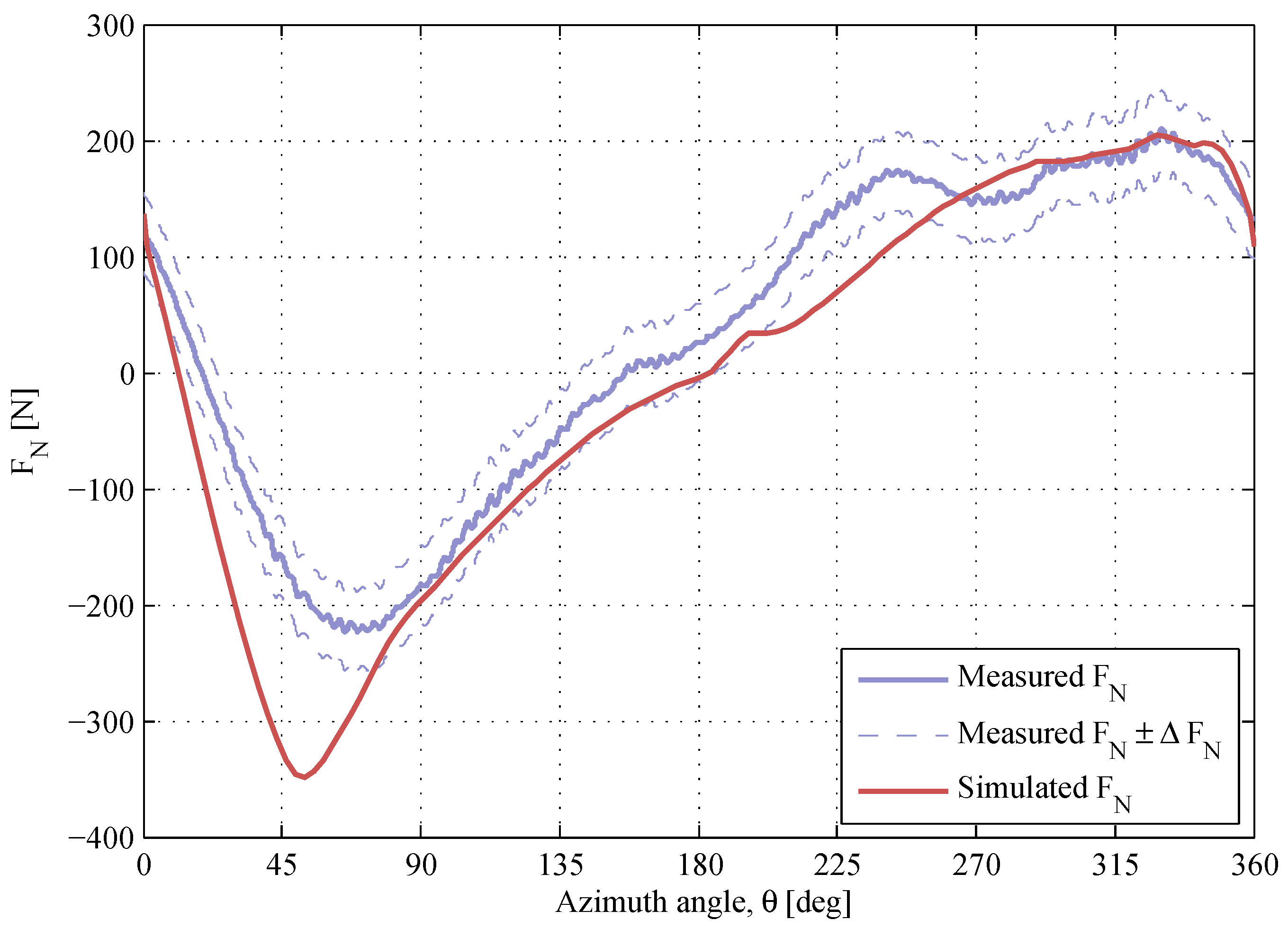
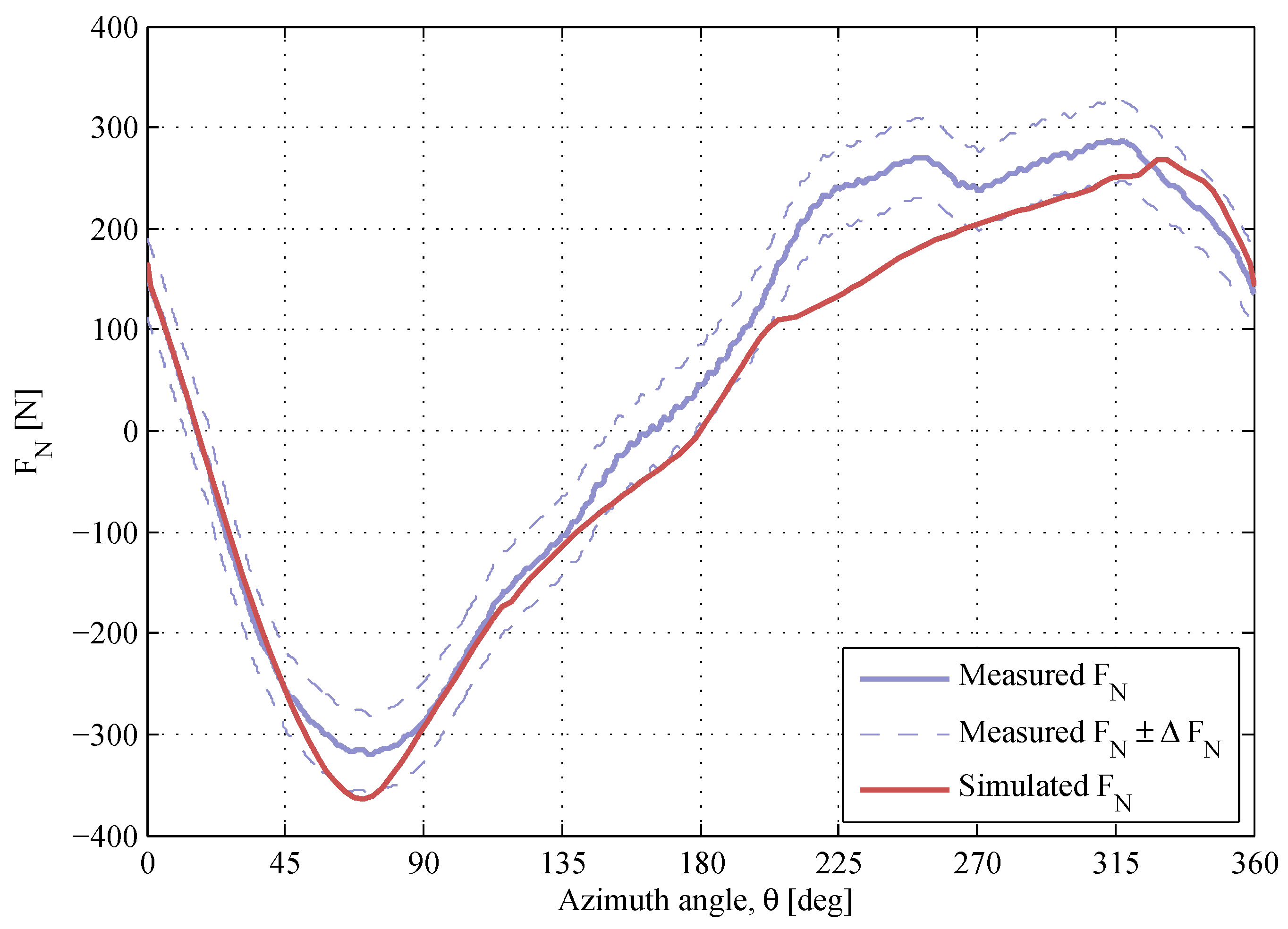
The normal force response at low TSRs is presented in Figure 9, Figure 10 and Figure 11. The maximum magnitude of the $F_N$-response at the upwind is overestimated at $\lambda =1.84$ and $\lambda =2.26$, and the shape of the modeled $F_N$-curve at the downwind deviates from the measurements. The authors presume that the difference between the simulated and the measured values at these low TSRs is due to high magnitudes of the angle of attack. The accuracy of the dynamic stall model decreases with increased angle of attack, which is shown in [25,29], where the dynamic stall model was tested against wind tunnel data for a single blade. As the angle of attack increases with decreased TSR, it is expected that the accuracy of the dynamic stall model should be limited at low TSRs. There is a positive offset of $F_N$ at $\theta =0^{°}$, which is mainly due to the blade pitch angle, which was chosen to even out the magnitude of α between the upwind and the downwind regions [18]. The value of the simulated $F_N$-offset is close to the measured one.

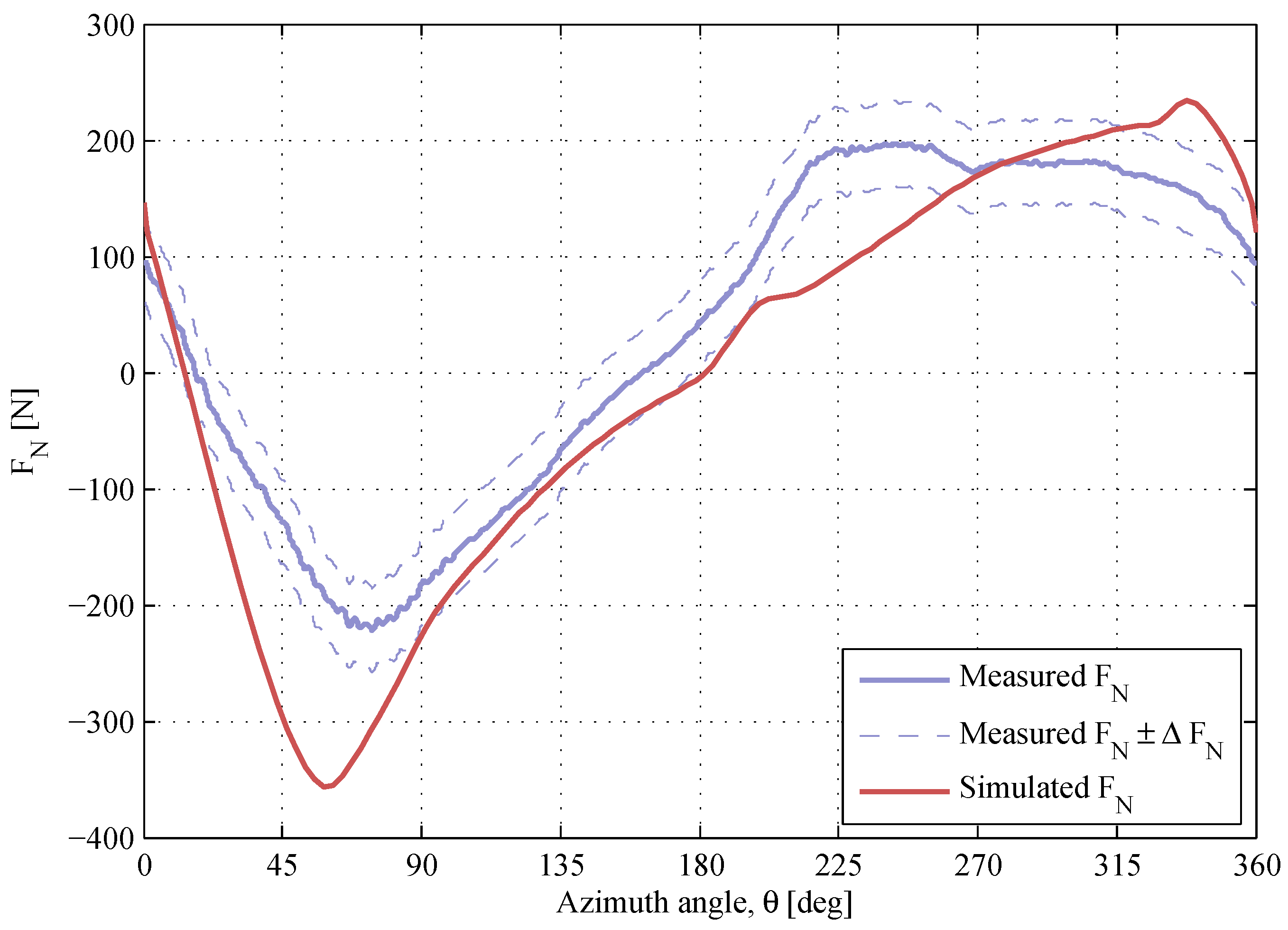
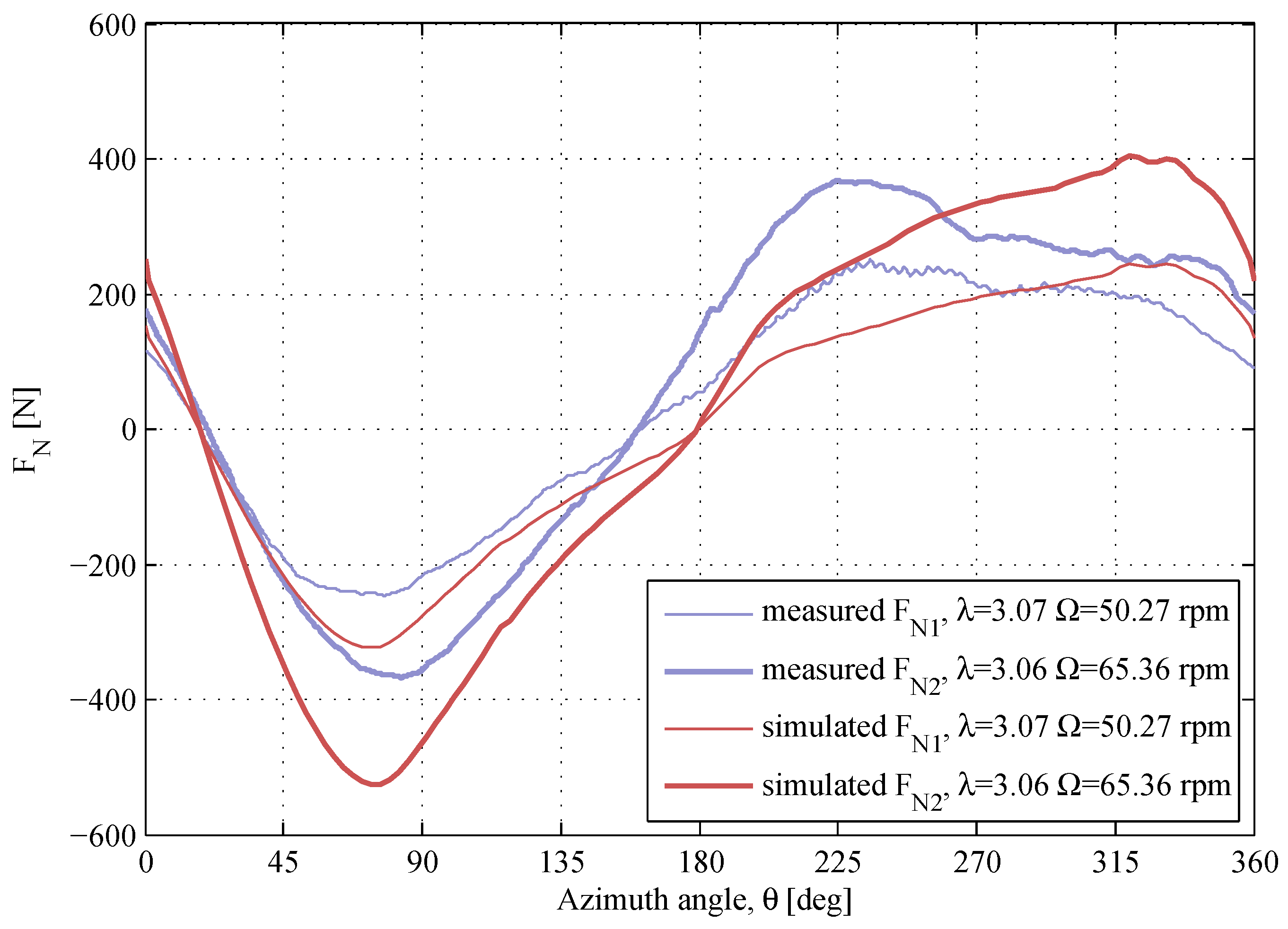
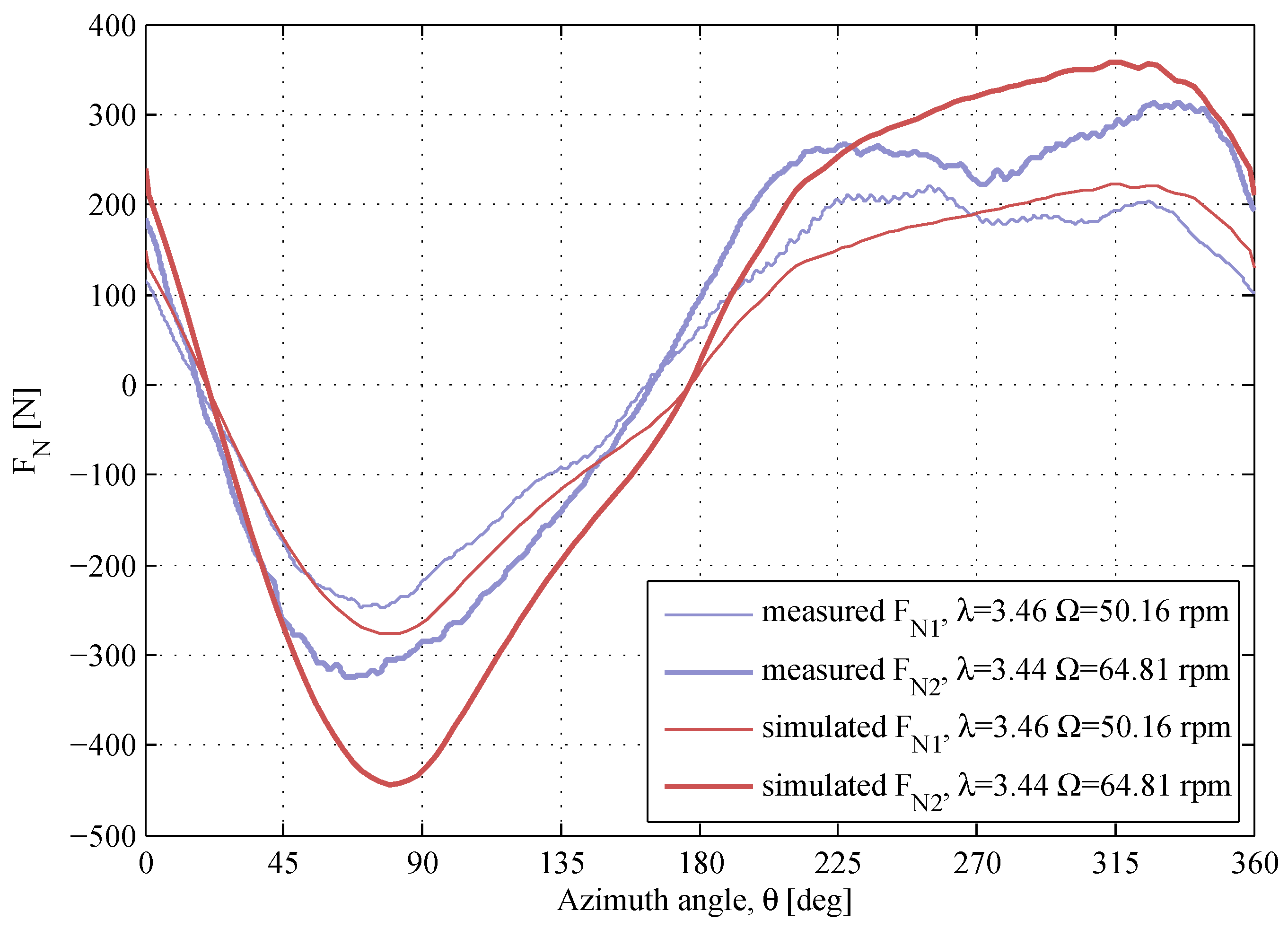
Figure 12 shows the $F_N$-response at $\lambda \approx 3$ for two different rotational speeds. The maximum magnitude of the $F_N$-curve is overestimated for $\Omega =65\mathrm{rpm}$, similarly to the overestimation in Figure 9 and Figure 10. The $F_N$-response at $\lambda \approx 3.45$ for $\Omega =50\mathrm{rpm}$ and $\Omega =65\mathrm{rpm}$ is presented in Figure 13. The results at these conditions are very similar to the results at $\lambda \approx 3$, although the model agrees better with experimental data at $\lambda \approx 3.45$. The measured $F_N$-response at $\lambda =3.44$ at $\Omega =65\mathrm{rpm}$ has a drop in the downwind region at ${225}^{°}<\theta <{325}^{°}$, which is not predicted by the model. The discussions regarding the $F_N$-drop are found further in this section.

Figure 9. The normal force at $\lambda =1.84$, $\Omega =40.29\mathrm{rpm}$. The air density and the kinematic viscosity are $\rho =1.25\mathrm{kg}/{\mathrm{m}}^3$ and $\nu =1.42·{10}^{-5}{\mathrm{m}}^2/\mathrm{s}$.

Figure 9. The normal force at $\lambda =1.84$, $\Omega =40.29\mathrm{rpm}$. The air density and the kinematic viscosity are $\rho =1.25\mathrm{kg}/{\mathrm{m}}^3$ and $\nu =1.42·{10}^{-5}{\mathrm{m}}^2/\mathrm{s}$.

Figure 10. The normal force at $\lambda =2.26$, $\Omega =45.19\mathrm{rpm}$. The air density and the kinematic viscosity are $\rho =1.25\mathrm{kg}/{\mathrm{m}}^3$ and $\nu =1.42·{10}^{-5}{\mathrm{m}}^2/\mathrm{s}$.

Figure 10. The normal force at $\lambda =2.26$, $\Omega =45.19\mathrm{rpm}$. The air density and the kinematic viscosity are $\rho =1.25\mathrm{kg}/{\mathrm{m}}^3$ and $\nu =1.42·{10}^{-5}{\mathrm{m}}^2/\mathrm{s}$.

Figure 11. The normal force at $\lambda =2.85$, $\Omega =50.80\mathrm{rpm}$. The air density and the kinematic viscosity are $\rho =1.27\mathrm{kg}/{\mathrm{m}}^3$ and $\nu =1.39·{10}^{-5}{\mathrm{m}}^2/\mathrm{s}$.

Figure 11. The normal force at $\lambda =2.85$, $\Omega =50.80\mathrm{rpm}$. The air density and the kinematic viscosity are $\rho =1.27\mathrm{kg}/{\mathrm{m}}^3$ and $\nu =1.39·{10}^{-5}{\mathrm{m}}^2/\mathrm{s}$.

Figure 12. The normal forces at similar λ and different Ω. The air densities and the kinematic viscosities are ${\rho }_1=1.27\mathrm{kg}/{\mathrm{m}}^3$, ${\rho }_2=1.24\mathrm{kg}/{\mathrm{m}}^3$ and ${\nu }_1=1.39·{10}^{-5}{\mathrm{m}}^2/\mathrm{s}$, ${\nu }_2=1.45·{10}^{-5}{\mathrm{m}}^2/\mathrm{s}$.

Figure 12. The normal forces at similar λ and different Ω. The air densities and the kinematic viscosities are ${\rho }_1=1.27\mathrm{kg}/{\mathrm{m}}^3$, ${\rho }_2=1.24\mathrm{kg}/{\mathrm{m}}^3$ and ${\nu }_1=1.39·{10}^{-5}{\mathrm{m}}^2/\mathrm{s}$, ${\nu }_2=1.45·{10}^{-5}{\mathrm{m}}^2/\mathrm{s}$.

Figure 13. The normal forces at the similar λ and different Ω. The air densities and the kinematic viscosities are ${\rho }_1=1.28\mathrm{kg}/{\mathrm{m}}^3$, ${\rho }_2=1.24\mathrm{kg}/{\mathrm{m}}^3$ and ${\nu }_1=1.39·{10}^{-5}{\mathrm{m}}^2/\mathrm{s}$, ${\nu }_2=1.45·{10}^{-5}{\mathrm{m}}^2/\mathrm{s}$.

Figure 13. The normal forces at the similar λ and different Ω. The air densities and the kinematic viscosities are ${\rho }_1=1.28\mathrm{kg}/{\mathrm{m}}^3$, ${\rho }_2=1.24\mathrm{kg}/{\mathrm{m}}^3$ and ${\nu }_1=1.39·{10}^{-5}{\mathrm{m}}^2/\mathrm{s}$, ${\nu }_2=1.45·{10}^{-5}{\mathrm{m}}^2/\mathrm{s}$.

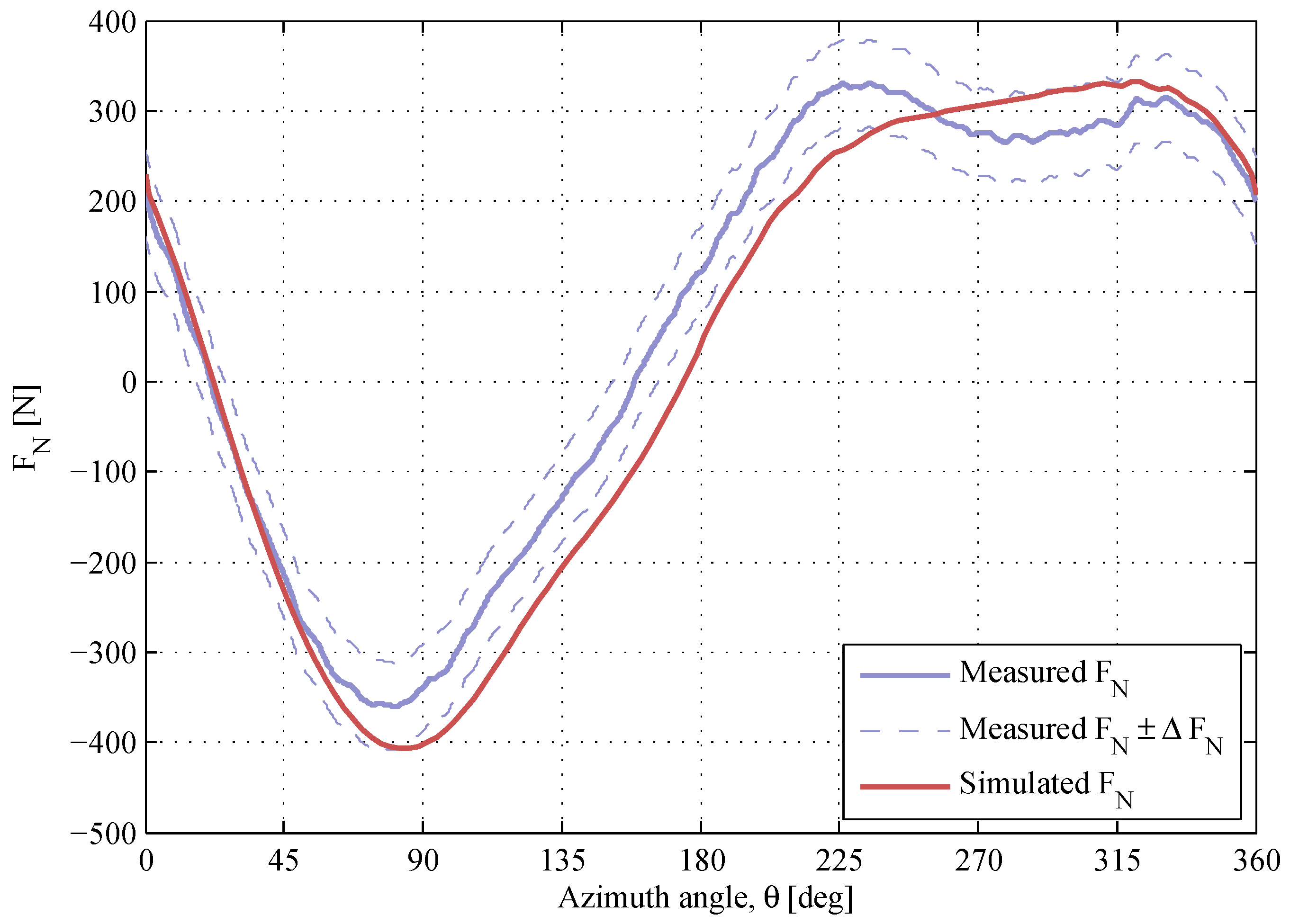
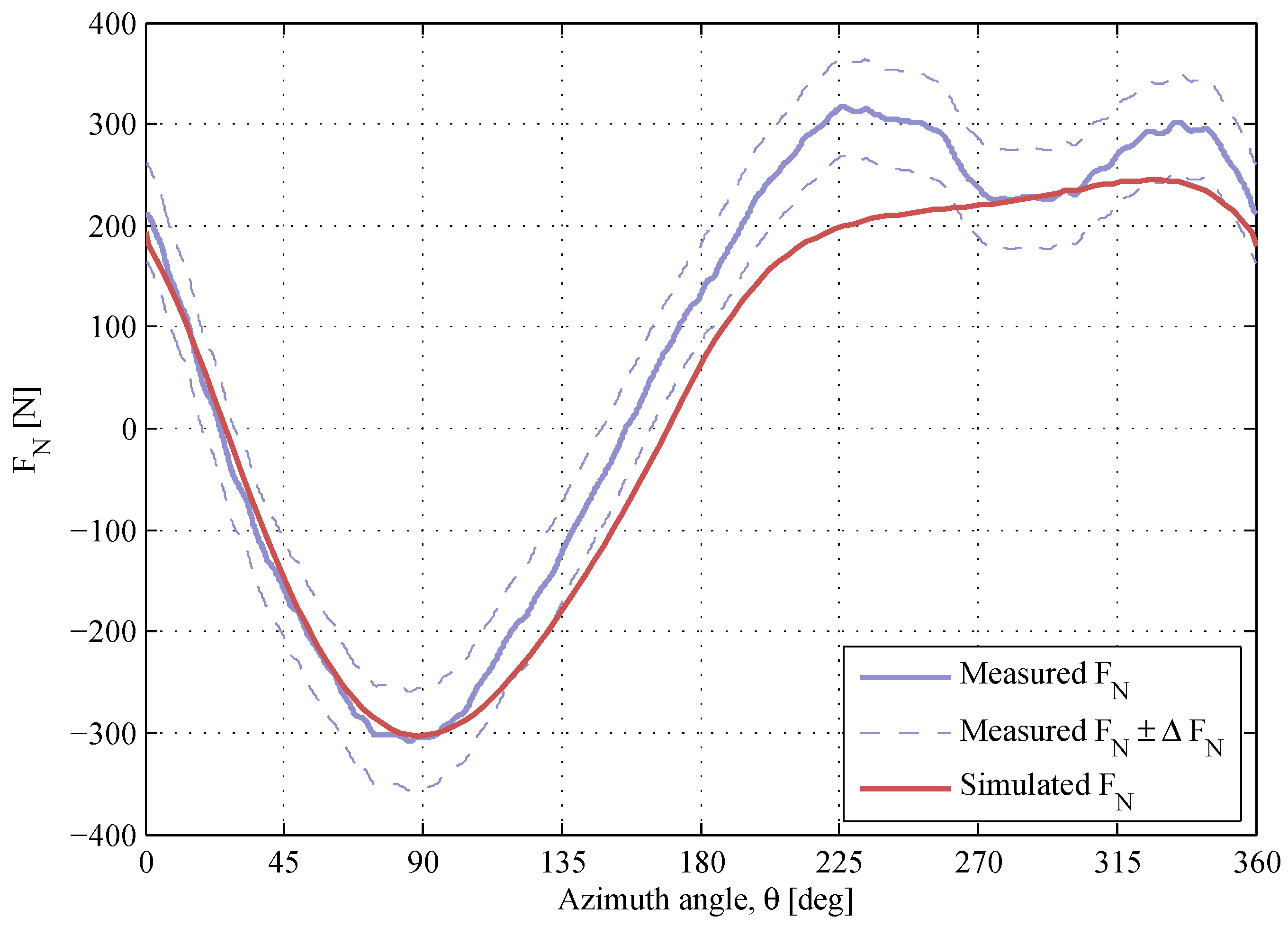
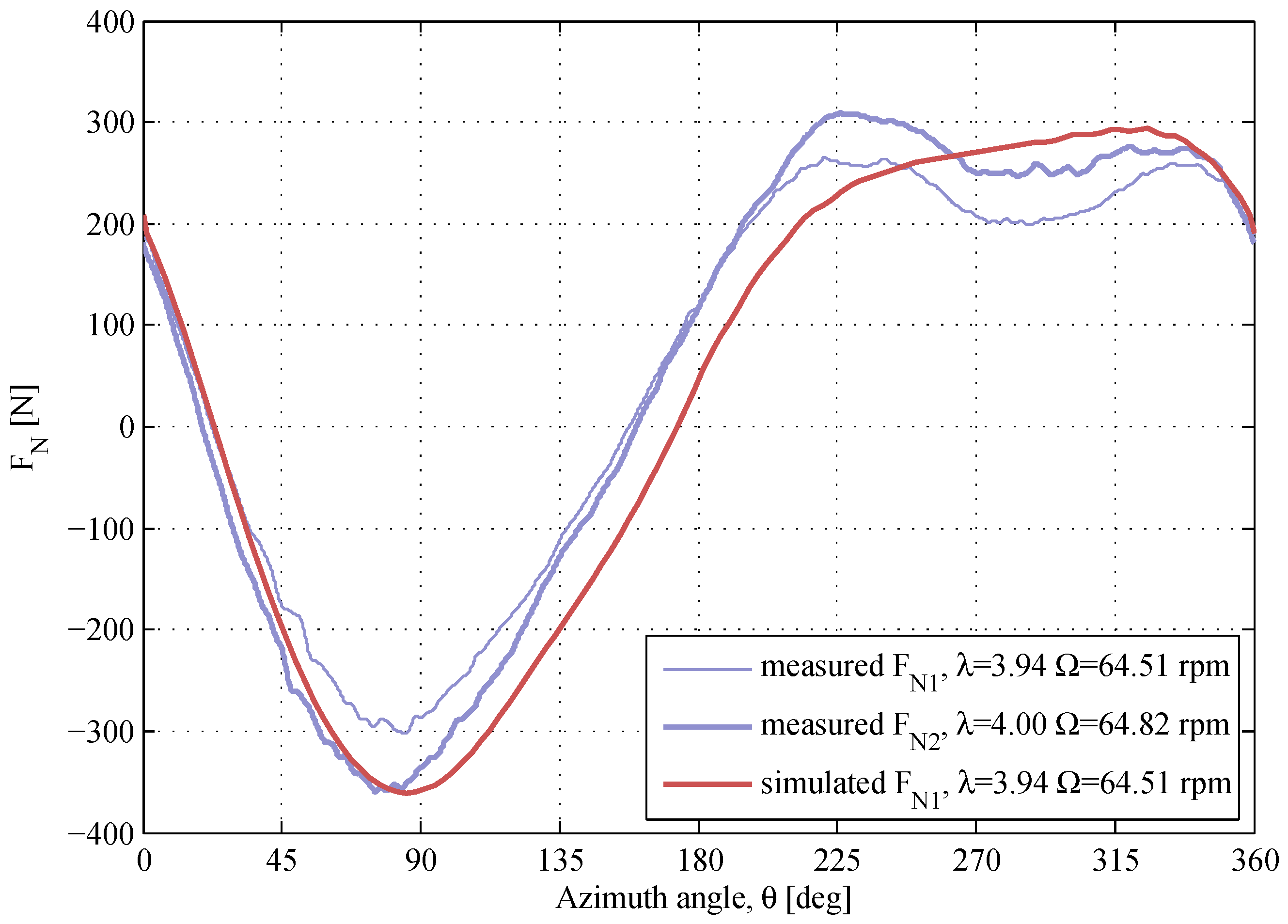
As the TSR increases, the maximum magnitude of the angle of attack decreases and the prediction of the blade forces becomes more accurate. The $F_N$-response at $\lambda =3.74$ is shown in Figure 14. The simulated data are in a good agreement with the measured data except the $F_N$-drop at ${235}^{°}<\theta <{330}^{°}$, which is missed by the model. The $F_N$-response at $\lambda =3.88$ for two different rotational speeds is shown in Figure 15. For both $F_N$-curves, the $F_N$-drop in the downwind is not predicted.

Figure 14. The normal force at $\lambda =3.74$, $\Omega =65.07\mathrm{rpm}$. The air density and the kinematic viscosity are $\rho =1.24\mathrm{kg}/{\mathrm{m}}^3$ and $\nu =1.44·{10}^{-5}{\mathrm{m}}^2/\mathrm{s}$.

Figure 14. The normal force at $\lambda =3.74$, $\Omega =65.07\mathrm{rpm}$. The air density and the kinematic viscosity are $\rho =1.24\mathrm{kg}/{\mathrm{m}}^3$ and $\nu =1.44·{10}^{-5}{\mathrm{m}}^2/\mathrm{s}$.

Figure 15. The normal forces at the similar λ and different Ω. The air densities and the kinematic viscosities are ${\rho }_1=1.28\mathrm{kg}/{\mathrm{m}}^3$, ${\rho }_2=1.24\mathrm{kg}/{\mathrm{m}}^3$ and ${\nu }_1=1.39·{10}^{-5}{\mathrm{m}}^2/\mathrm{s}$, ${\nu }_2=1.43·{10}^{-5}{\mathrm{m}}^2/\mathrm{s}$.

Figure 15. The normal forces at the similar λ and different Ω. The air densities and the kinematic viscosities are ${\rho }_1=1.28\mathrm{kg}/{\mathrm{m}}^3$, ${\rho }_2=1.24\mathrm{kg}/{\mathrm{m}}^3$ and ${\nu }_1=1.39·{10}^{-5}{\mathrm{m}}^2/\mathrm{s}$, ${\nu }_2=1.43·{10}^{-5}{\mathrm{m}}^2/\mathrm{s}$.

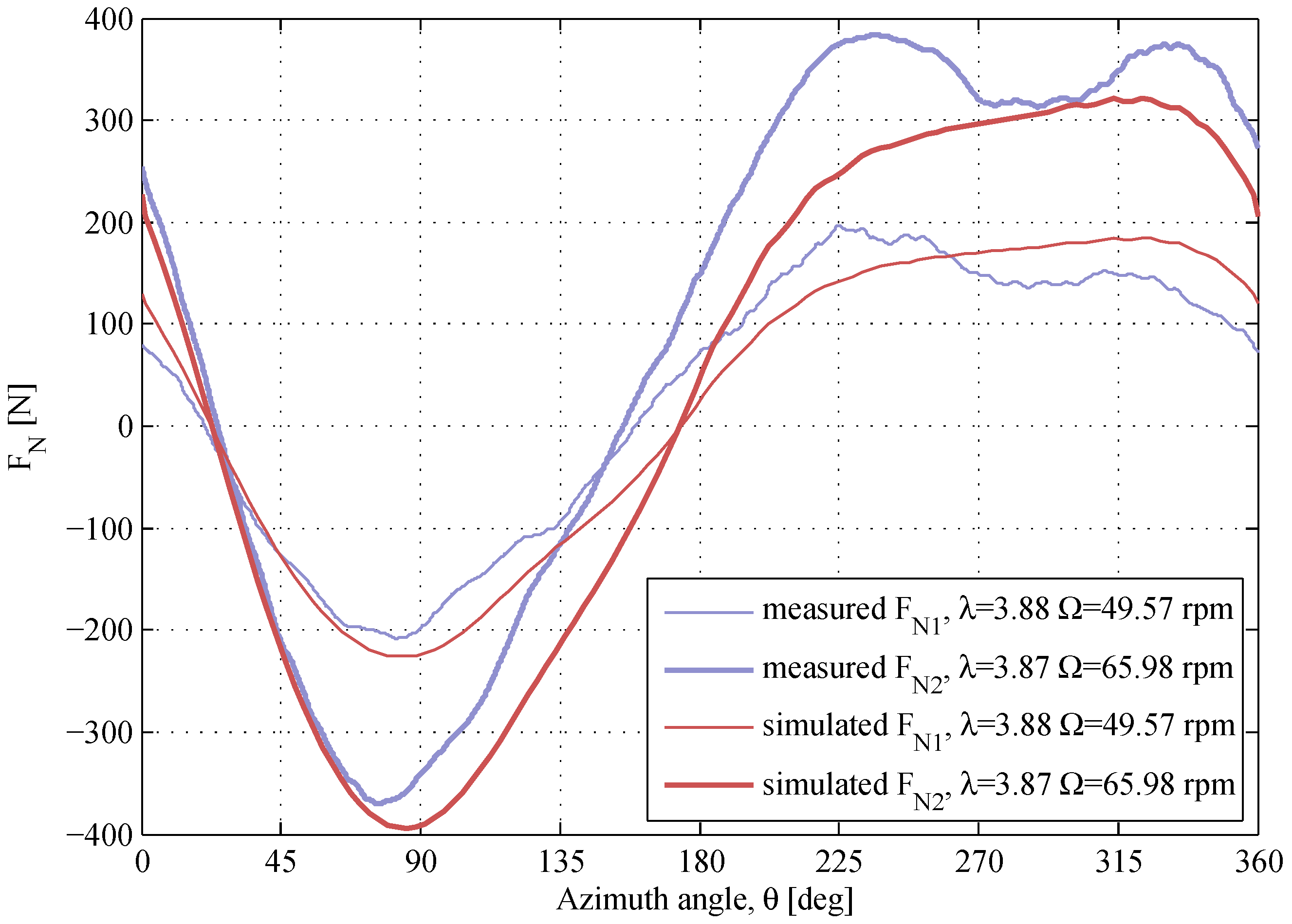
Two sets of the experimental data with almost identical operational conditions are compared against the simulated results in Figure 16. The shape of the measured $F_N$-curves is matching, but the magnitudes are slightly different. The maximum difference in the measured $F_N$ magnitudes is $\sim 50\mathrm{N}$, though the TSR is almost identical (${\lambda }_1=3.94$ and ${\lambda }_2=4.00$), and the difference in the air density is minor (see the notation to Figure 16). The model shows a close agreement, except that the $F_N$-drop at the downwind is not present.

Figure 16. The normal forces for two different sets of data with almost identical λ and Ω. The air densities and the kinematic viscosities are ${\rho }_1=1.24\mathrm{kg}/{\mathrm{m}}^3$, ${\rho }_2=1.24\mathrm{kg}/{\mathrm{m}}^3$ and ${\nu }_1=1.44·{10}^{-5}{\mathrm{m}}^2/\mathrm{s}$, ${\nu }_2=1.45·{10}^{-5}{\mathrm{m}}^2/\mathrm{s}$.

Figure 16. The normal forces for two different sets of data with almost identical λ and Ω. The air densities and the kinematic viscosities are ${\rho }_1=1.24\mathrm{kg}/{\mathrm{m}}^3$, ${\rho }_2=1.24\mathrm{kg}/{\mathrm{m}}^3$ and ${\nu }_1=1.44·{10}^{-5}{\mathrm{m}}^2/\mathrm{s}$, ${\nu }_2=1.45·{10}^{-5}{\mathrm{m}}^2/\mathrm{s}$.

The results at the TSR of 4.6 are presented in Figure 17. At this high TSR, the flow expansion strongly affects the turbine aerodynamics. The model underestimates the maximum magnitude of the $F_N$-response in the downwind region. The aforementioned $F_N$-drop at the downwind is clearly observed at $\lambda =4.6$, and the model misses it.

Figure 17. The normal force at $\lambda =4.57$, $\Omega =65.35\mathrm{rpm}$. The air density and the kinematic viscosity are $\rho =1.25\mathrm{kg}/{\mathrm{m}}^3$ and $\nu =1.43·{10}^{-5}{\mathrm{m}}^2/\mathrm{s}$.

Figure 17. The normal force at $\lambda =4.57$, $\Omega =65.35\mathrm{rpm}$. The air density and the kinematic viscosity are $\rho =1.25\mathrm{kg}/{\mathrm{m}}^3$ and $\nu =1.43·{10}^{-5}{\mathrm{m}}^2/\mathrm{s}$.

General Discussion

The presented simulations are in 2D, while the measured data are in 3D, and the contribution of the support arms is included in the measured forces. Therefore, it is expected that the presented model cannot reproduce the experimental results in great detail, especially where 3D effects are strong. The flow expansion in the simulation model is limited to the horizontal plane only, and the vertical expansion is omitted. This error should be most prominent at high TSRs, where the flow expansion is largest. Additionally, the current 2D model will not capture wind shear, which would cause a variation of the flow velocity, and hence, the TSR over the turbine height.

Over the whole range of the presented data, the model performs better in the upwind side. This is expected, since the dynamic stall vortex is not implemented in the flow field and the wake effects should be smaller in the upwind side. Furthermore, since the support arms are not included in the model, collision of the blade with vortices from the support arms cannot be reproduced. This is a possible contributing factor to the $F_N$-drop at $\lambda >3.4$, as the support arms can have a notable contribution to the wake. The $F_N$-drop is not expected to be due to the tower wake, since the tower diameter is considerably smaller than the region of the $F_N$-drop. This drop can also be caused by other three-dimensional effects, such as tip vortices, which are not included in the current model.

There are limitations of the dynamic stall model itself: it is assumed that the blade is a flat plate, and the flow velocity is constant during the change of the angle of attack [29]. Additionally, flow curvature is represented only through a correction in the angle of attack, while it can also influence the empirical constants of the dynamic stall model. These limitations should be considered when evaluating the performance of the model.

The maximum measurement error is estimated for every $F_N$-curve using Equation (5). Due to the high repeatability of the measured normal force, the shape of the $F_N$-curve is likely to remain, though the measurement error can change the scale of the $F_N$-response. This is observed when comparing two sets of data at almost identical operational conditions; Figure 16. Therefore, the measurement error has to be considered throughout the assessment of the simulation model.

The major advantage of the presented model is its computational speed: one simulation with 100 revolutions is in the order of minutes on a single core machine, which is much faster than simulations with 2D CFD models. A 3D vortex model does not have the previously-mentioned constraints with the flow expansion modeling and with the implementation of the support arms. However, the computational time of the existing 3D vortex models is still high, and the computational time of 3D CFD models can be a few months [1]. In this light, the presented simulation model can be used for the fast dimensioning of the turbine loads.

5. Conclusions

A two-dimensional vortex model for VAWTs was described. The simulation results on the normal forces were assessed against the new experimental data from the straight-bladed VAWT operated at an open site. The comparison is presented for a wide range of operational conditions. There is a drop in the normal force in the downwind region, which is more prominent at high TSR. The authors presume that this drop is due to three-dimensional effects, which are not implemented in the current model. The simulation model shows higher accuracy for the upwind region than for the downwind. At low TSRs, the model misses the measured results, which is expected to be due to the limitations of the dynamic stall model at the high magnitudes of the angle of attack. However, the simulated results agree well with the measured data at moderate and high TSRs, except the force drop in the downwind region. Although the model does not reproduce the experimental results in great detail, it shows a reasonable agreement with experimental data, and it can be used to simulate the maximum load limits on VAWTs at a low computational cost.