1. Introduction
The internal combustion engine (ICE) is a widely used and well-developed technology, however, pollution and energy resource issues are growing concerns. Hybrid vehicles (HVs) are an effective and common solution to these issues. Most manufacturers have developed hybrid electric vehicle (HEV) systems to improve vehicle fuel economy and cost. Energy management and emission control for electric and IC engine power systems have been studied and developed for various hybrid systems [
1,
2,
3,
4]. In a hybrid electric vehicle, energy management is important because it can substantially affect vehicle performance and component size. Several control strategies have been implemented in HEVs [
5]. Rule-based and fuzzy-based control strategies are widely used in light and medium-sized HEVs. Rule-based control is simpler but less flexible than fuzzy-based control. Fuzzy-based control can identify and learn driver behaviors under various driving conditions. Both strategies are applicable for real-time control [
6]. Although a dynamic programming (DP) solution can numerically optimize a specific drive-cycle [
7,
8], stochastic dynamic programming (SDP) can optimize solutions for assumed road-load conditions with known probabilities [
9]. Studies of heuristic rule-base methods [
10,
11] and experiments in fuzzy logic control (FLC) with an intelligent supervisory control strategy suggest that refined ICE speed transitions are also good candidates for implementation in control algorithms. Another configuration of hybrid vehicle is the hydraulic hybrid vehicle (HHV), in which a hydraulic pump replaces the electric motor as the primary or assistant driving power and the accumulator replaces the battery for energy storage. The hydraulic hybrid system provides large power capacity and more suitable for heavy duty vehicle [
12,
13]. Compared to HEVs, HHVs recapture more energy during braking, and it makes the HHV more suitable for urban driving applications which include frequent stops and starts [
14,
15,
16]. New energy management strategies have been proposed to improve fuel efficiency [
17,
18].
Generally, conventional manual or automatic transmissions are used to regulate an engine within a certain range of engine speeds and to output rotational speed and torsional moments according to driver demands. The main disadvantage of these transmissions is their dependence on a gearbox for gearshift actions. During gearshifts, sudden changes in engine speed, which are common in conventional gearboxes, produce discontinuities in gear-shifting. Hydraulic transmission systems provide variable speed ratios between engine and wheels which remove the sudden changes during the gear-shifting. Continuously variable transmissions (CVTs) also are unaffected by gearshift discontinuities during the shifting process, thus providing passengers with a comfortable and uninterrupted ride. The advantage of the CVT is that by minimizing the power loss of an engine, engines can operate at peak efficiency or at constant engine speeds. Moreover, CVTs are structurally simple and easily maintained. However, CVTs cannot withstand excessive frictional forces generated by the torsional moments of engines because of limited belt or chain strengths. Therefore, hydraulic transmission systems have the following advantages over CVTs:
- (1)
Steady transmission: Hydraulic transmission devices operate by using hydraulic oil, which is nearly incompressible at ordinary pressures and using continuously flowing hydraulic oil to make gearshifts. Because hydraulic oil has shock absorbing capacities, hydraulic buffer devices can be installed in the oil lines to provide steadily operating transmissions.
- (2)
Light weight and compact size: In contrast to mechanical and electrical transmissions, hydraulic transmissions are substantially lighter and smaller under identical output power conditions. Thus, hydraulic transmissions have low inertia and are highly responsive.
- (3)
High capacity: Hydraulic transmissions can readily receive large forces and torsional moments.
- (4)
Readily obtainable infinitely variable speeds: In hydraulic transmissions, infinitely variable speeds can be obtained by regulating fluid flow rates. The adjustment ratio can vary widely from 1:1 to 2000:1. Extremely low speeds are easily achieved.
Regarding vehicle transmission systems, hydraulic transmission systems can achieve similar continuously variable speed functions. In principle, hydraulic pumps convert mechanical energy provided by engines into fluid hydraulic energy. Finally, hydraulic motors convert high pressure hydraulic energy into mechanical energy to drive the vehicles. To obtain continuously variable speed functions, only the hydraulic motor or hydraulic pump valve opening must be adjusted. This system provides continuously variable and broad gear reduction ratios. However, hydraulic motors and pumps that operate at high pressures and small openings are usually inefficient.
Hydraulic systems have a high pressure accumulator for energy storage and hydraulic pumps/motors to transfer power and are often used for heavy duty vehicles in the past. Recently, the applications can be seen in the passenger or light duty vehicles. Sizes of the hydraulic systems are applicable for the stop-start operation. The accumulator has high power density, can be completely charged and discharged for many cycles and constantly switched between charging and discharging states without being concerned about functional degradation or capacity loss. All these features make hydraulic systems very attractive for stop-start operation, especially in city driving.
Many studies have been done for Manual Transmission Vehicles, Series Hybrid Electric Vehicles, Parallel Hybrid Electric Vehicles, and Electric Vehicles. Growing interest in Series Hydraulic Hybrid Vehicles, Parallel Hydraulic Hybrid Vehicles, and Hydraulic-Electric Hybrid Vehicles can also be seen. However, most studies have focused on improving energy management strategies, improving designs for single configuration, or optimizing their components/subsystems efficiencies, such as hydraulic pumps/motors, DC motors, or batteries, etc., for given configurations. Energy control strategies have been specifically tailored to the particular systems or for special events or applications, and the improvement comparisons were made against their own baseline designs. Few studies have compared energy efficiency among different configurations of hydraulic hybrid vehicles and hybrid electric vehicle systems. Therefore, this research uses MATLAB Simulink to construct all seven complete models for backward simulations, evaluates the fuel economy with comprehensive comparison among all the listed systems, and discusses the suitable applications for different powertrain configurations. This research compares the energy efficiency based on New European Driving Cycle (NEDC) through various power component models, connection with energy storage component models, and combinations of series or parallel configurations, and concludes that hydraulic-electric hybrid vehicle (HEHV) have the highest cost efficiency among all the configurations studied.
2. System Modeling
This section introduces various model components. Methods and empirical equations were established for each component model. To compare the differences between the hydraulic hybrid vehicle (HHV) and hybrid electric vehicle (HEV) models, hydraulic subsystem models were established and comprised hydraulic pump, hydraulic motor, and accumulator models. This study also established models of electrical subsystems, including the electric motor, generator, and lithium-ion battery. Electrical subsystem models supply power to series and parallel HEVs (SHEVs and PHEVs), and pure electric vehicles (EVs), whereas hydraulic subsystem models supply power to series and parallel HHVs (SHHVs and PHHVs) and hydraulic–electric hybrid vehicles (HEHVs).
Table 1 presents the powertrain configurations and components applied in the research.
Table 1.
Vehicle Configurations.
Table 1.
Vehicle Configurations.
| Configuration/Components & Subsystems | Internal Combustion Engine | Electric System | Hydraulic System | Brake Regenerating | Parallel | Series |
|---|
| MT vehicle (manual transmission) | x | | | | | |
| Electric Vehicle | SHEV | x | x | | x | | x |
| PHEV | x | x | | x | x | |
| EV | | x | | x | | |
| Hydraulic Vehicle | SHHV | x | | x | x | | x |
| PHHV | x | | x | x | x | |
| HEHV | | x | x | x | x | |
Modeling was performed by backward simulation [
9]. The required speed-time relationships were entered into the model of driving cycles before running each simulation. In this study, vehicle speed follows the New European Driving Cycle (NEDC).
2.1. Driving Cycle Model
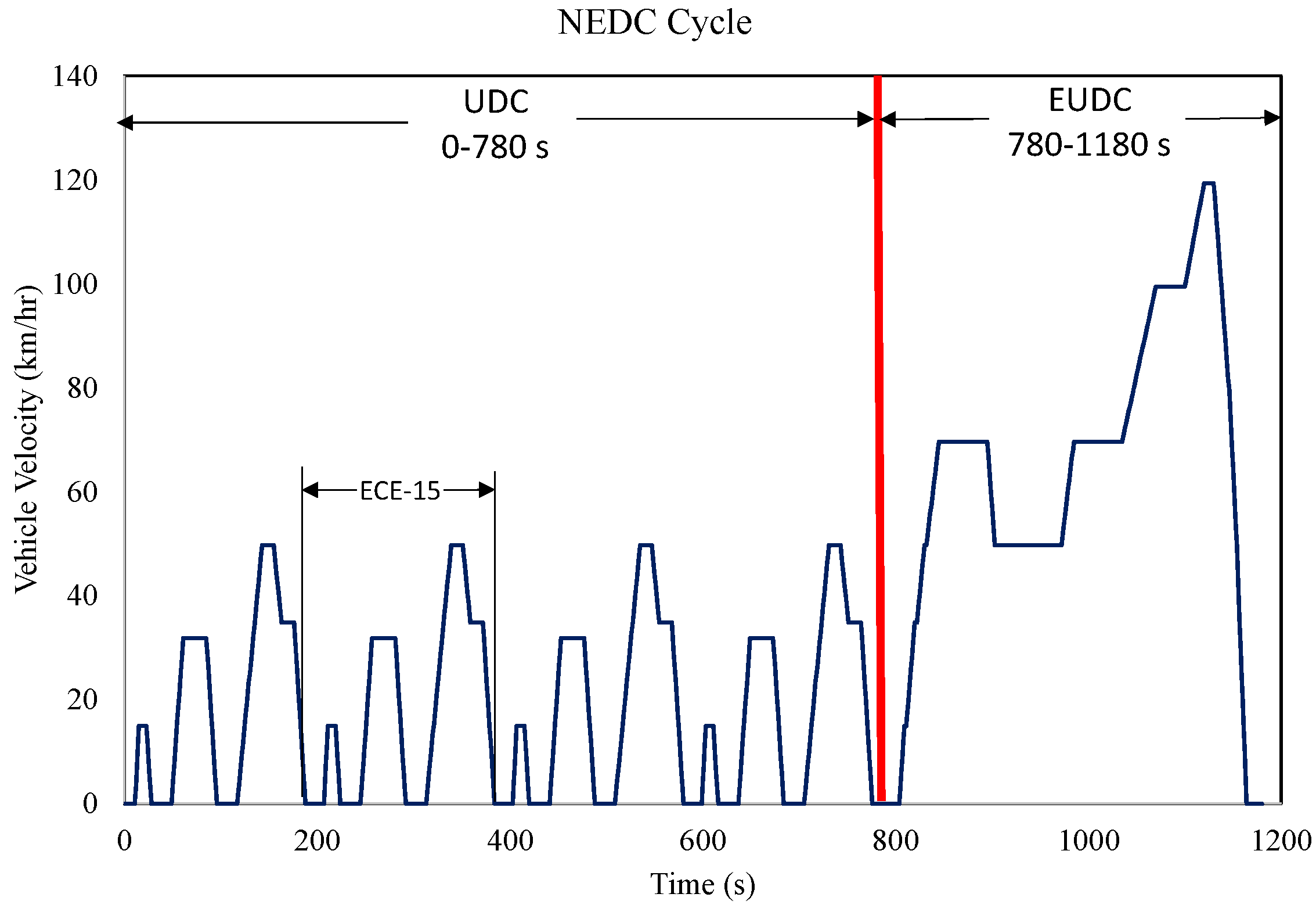
The entire simulation analysis began from the driving cycles based on the NEDC (
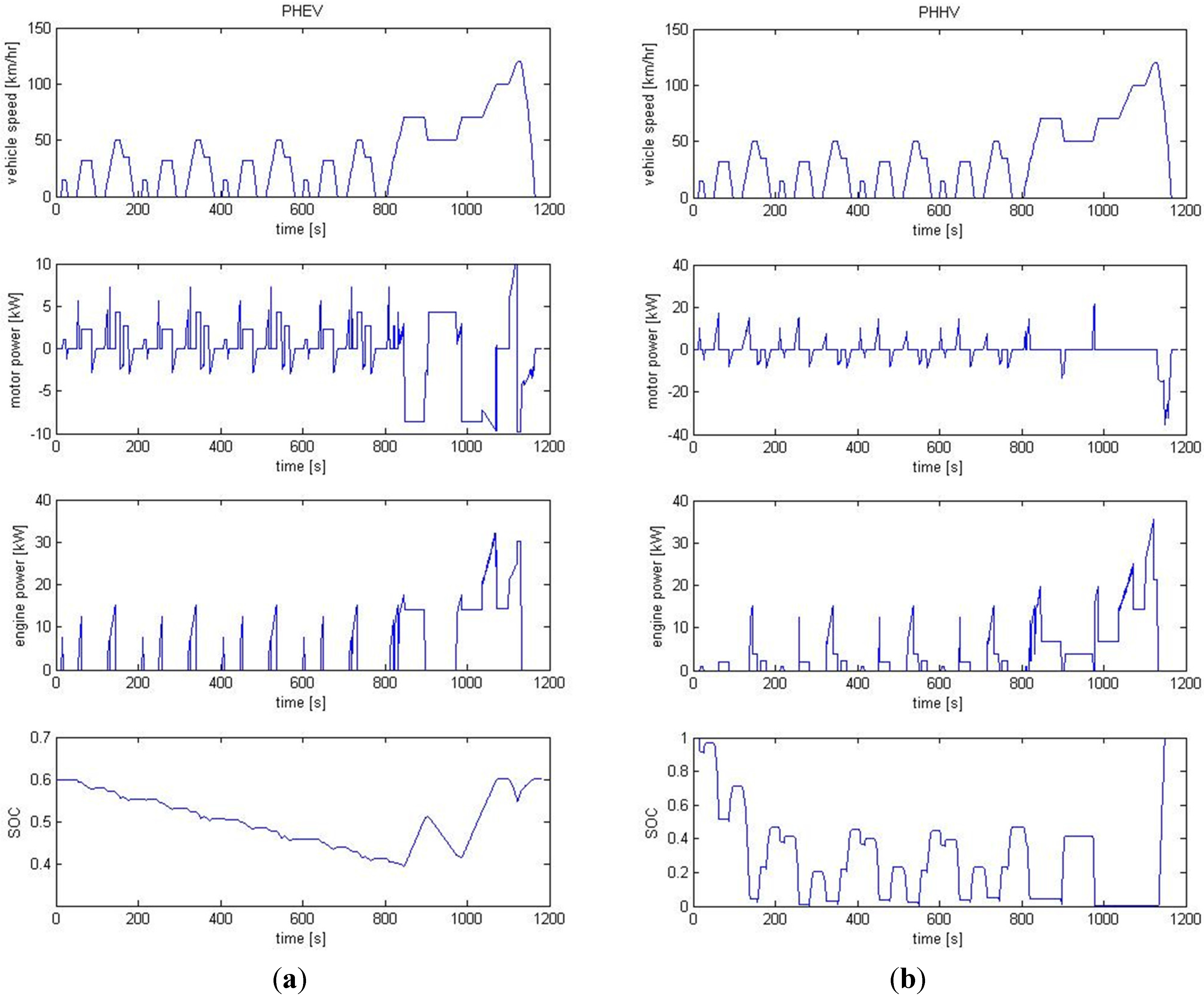
Figure 1) for standardized testing procedures to provide instantaneous driving forces required to overcome the aerodynamic, rolling, grade, and inertia resistances. The entire driving cycle (total time, 1180 s) including urban driving cycles (UDCs) and extra-urban driving cycles (EUDCs). The first 780 s was the UDC (maximum speed 50 km/h), and the next 400 s was the EUDC (maximum speed 120 km/h).
Figure 1.
NEDC driving cycle.
Figure 1.
NEDC driving cycle.
2.2. Vehicle Dynamic Model
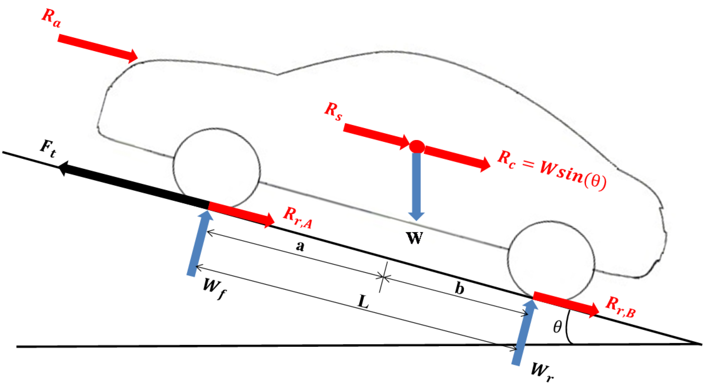
Figure 2 (red arrows) shows the vehicle driving resistances, including the rolling, aerodynamic, grade, and acceleration resistances. The vehicle driving forces are calculated through the dynamic vehicle model by using the following equations:
where
Ft is the tractive effort;
Rr is the rolling resistance; μ
r is the rolling resistance coefficient,
W is the vehicle weight;
Ra is the aerodynamic dragging force;
CD is the aerodynamic dragging coefficient;
v is vehicle speed;
vw is wind speed;
Rc is the grade resistance;
We is the equilibrium weight of rotational part;
a is vehicle acceleration; and
Rs is the inertia force. The grade was set to 0 in all fuel economy simulations.
Figure 2.
Vehicle dynamic analysis.
Figure 2.
Vehicle dynamic analysis.
2.3. Engine Model
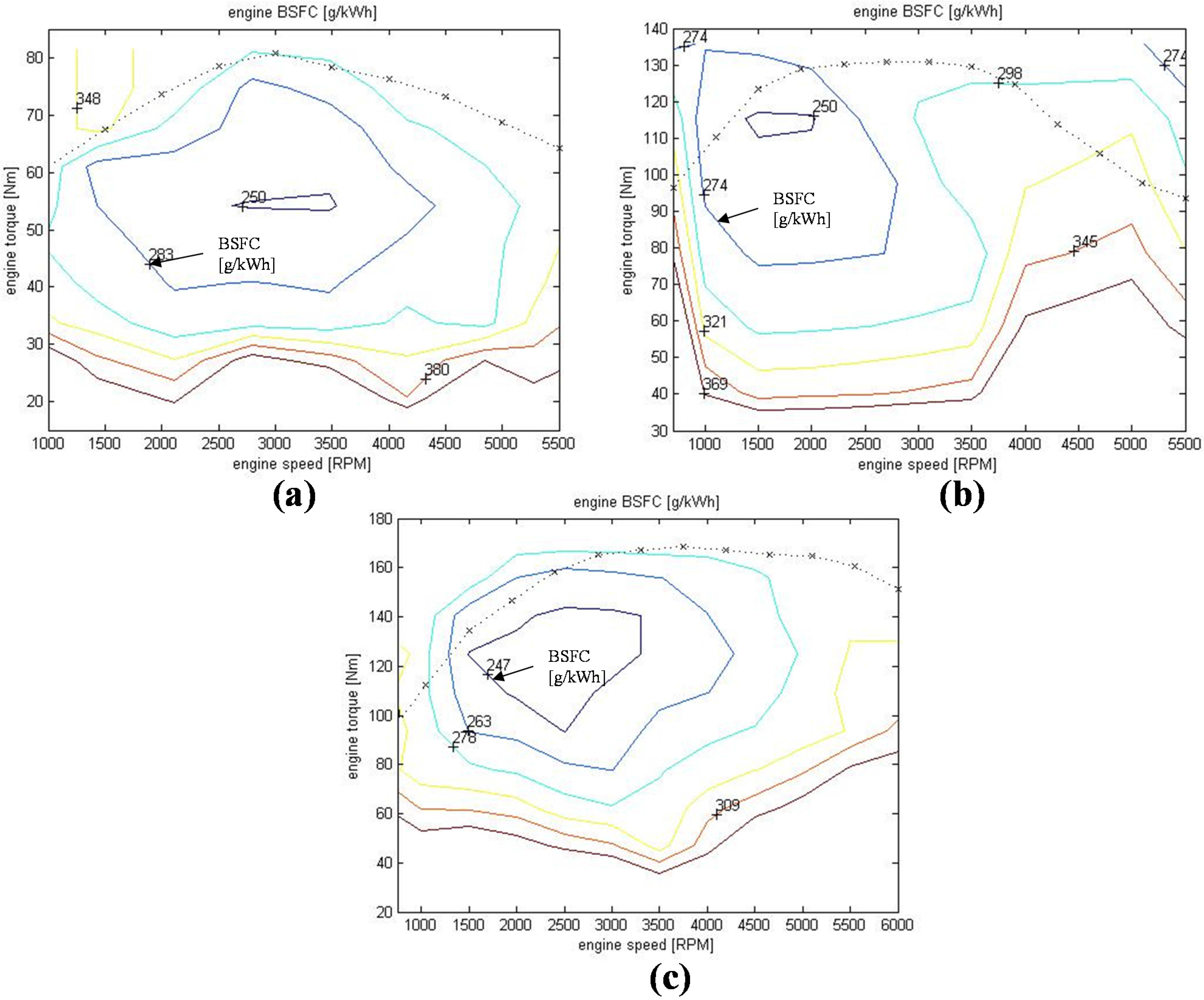
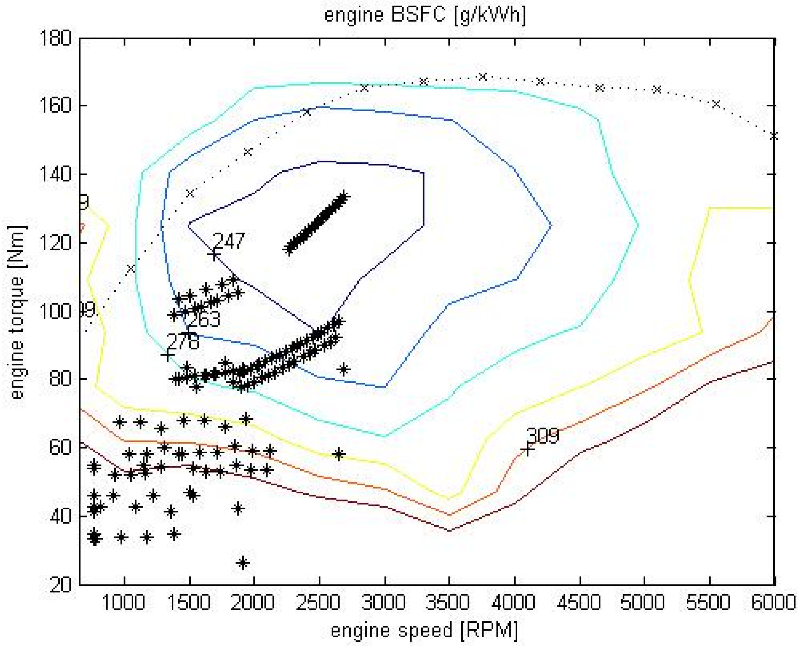
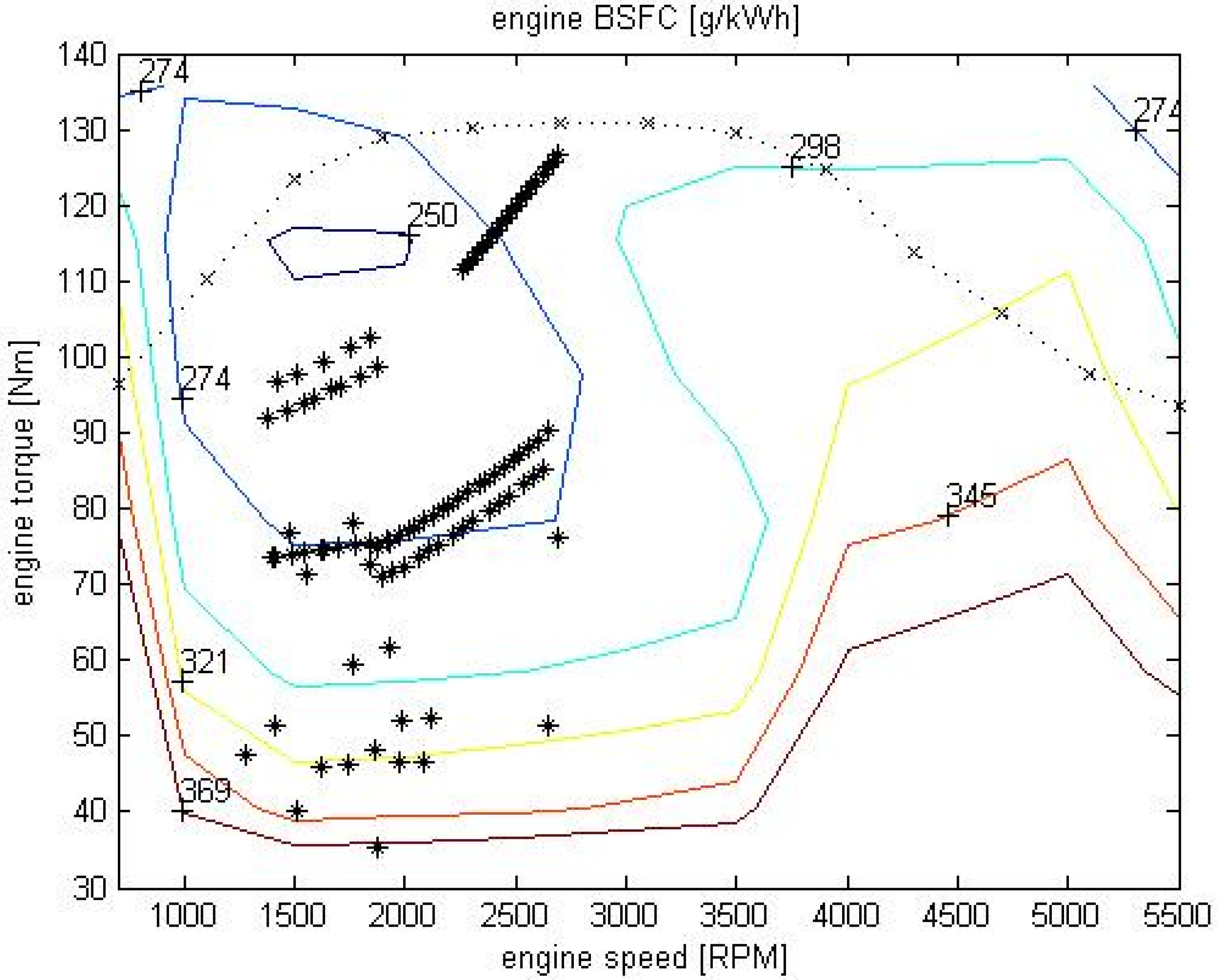
The engine model in this study was a steady state engine model. Vehicle fuel consumption is related to the engine operating conditions. Therefore, the speed and time required for the driving cycles is converted to engine speed and torque. The look-up table method was applied to obtain the brake specific fuel consumptions (BSFC) for the known engine speeds and engine torques and subsequently calculate the vehicle fuel consumptions. Engine specifications for series, parallel, and conventional vehicles were designed by dividing gasoline engines into three displacement volumes of 1.0, 1.3, and 1.8 L, which generate maximal powers of 41, 63, and 95 kW, respectively.
Figure 3 presents BSFC diagrams. The three engines were designed to be compatible with each basic configuration. The conventional manual transmission vehicle (MT) is equipped with a 1.8 L engine. The parallel hybrid systems, PHEV and PHHV, use a 1.3 L engine. Since they have an electric motor that assists driving power, their engine power can be lower than that of the MT vehicle. The series hybrid vehicles, which are driven by motors, use a 1.0 L engine. The engine is used to charge the battery. The average tractive power through the driving cycle is much lower than the peak power, therefore, the engine for series hybrid vehicles can be much smaller. The engine data in
Figure 3 were retrieved from the ADVISOR 2003 database [
19].
Figure 3.
The BSFC contour diagrams for (a) 41, (b) 63, and (c) 95 kW gasoline engines.
Figure 3.
The BSFC contour diagrams for (a) 41, (b) 63, and (c) 95 kW gasoline engines.
2.4. Power Component Model
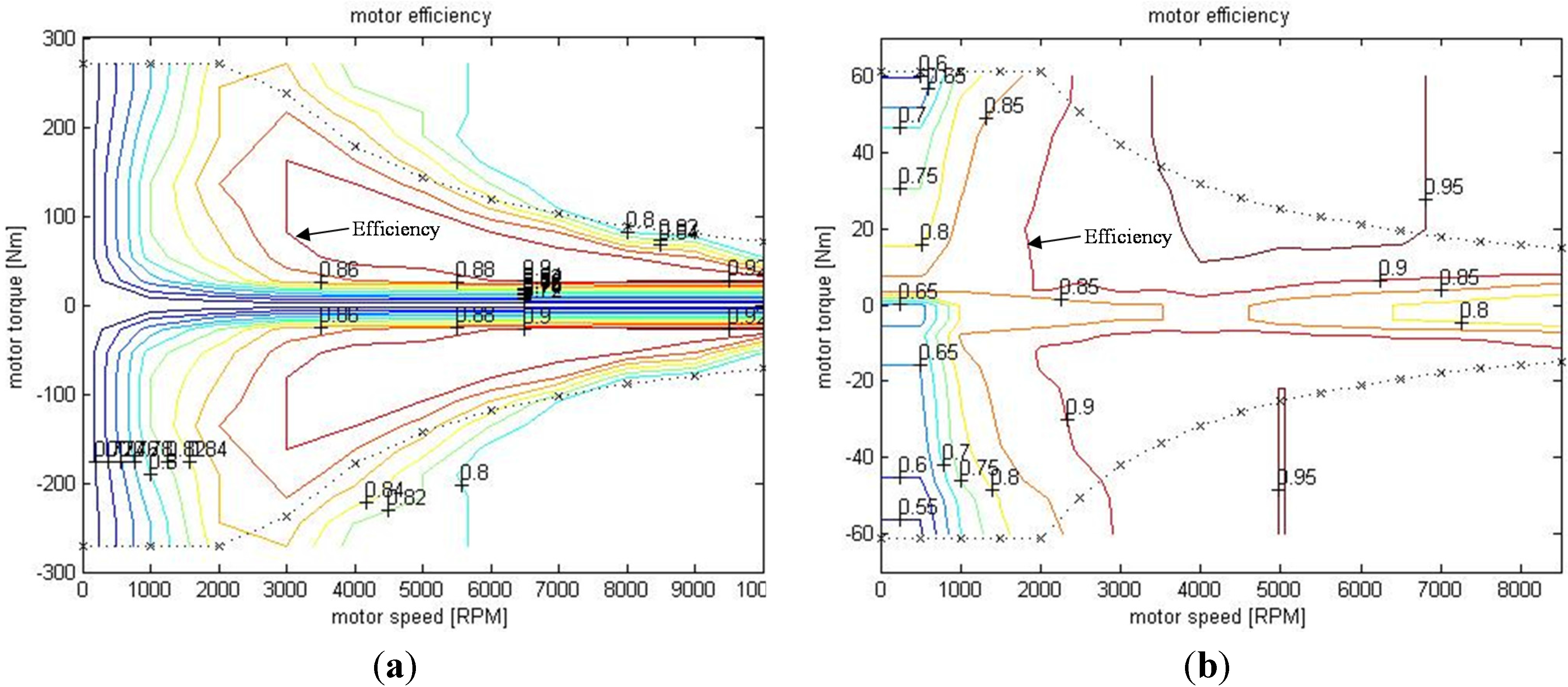
2.4.1. Electric Motor Model
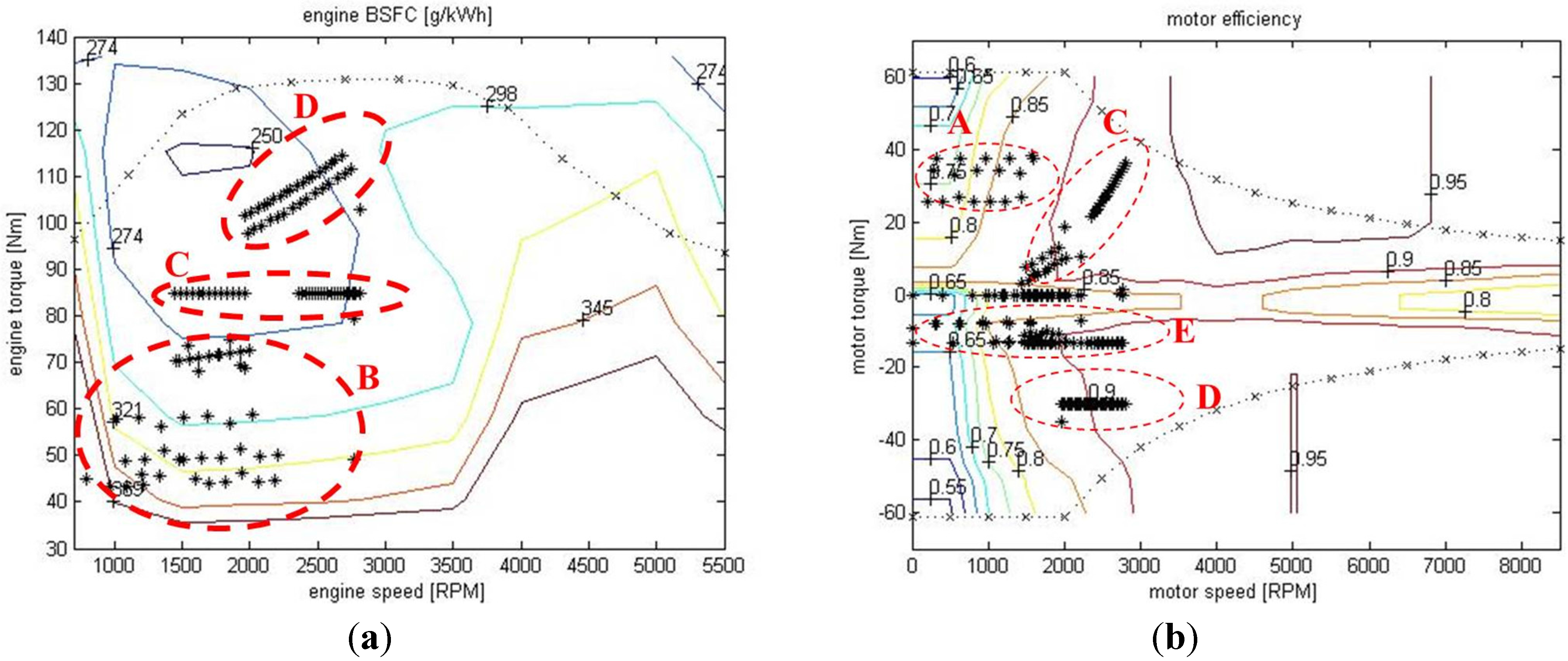
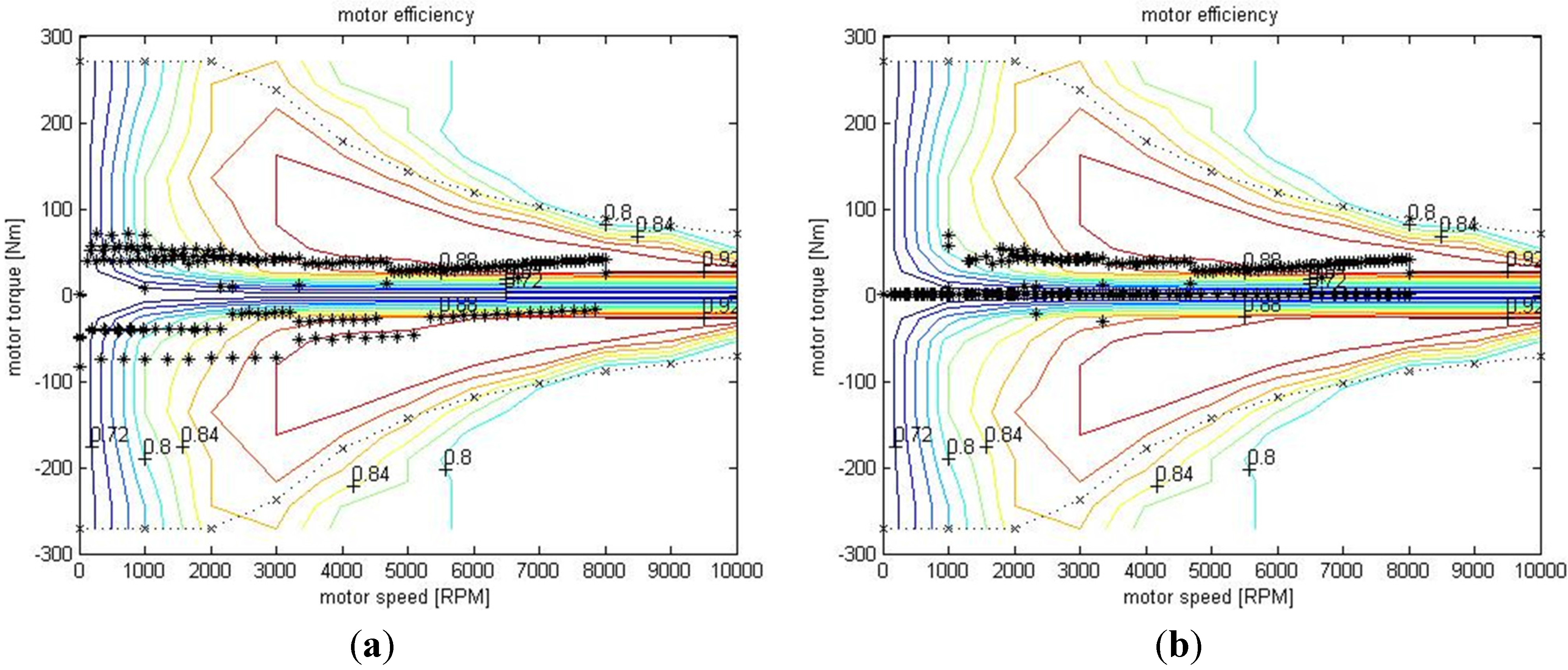
The electric motors were permanent magnet motors with outputs of 75 and 10 kW, which were used in the series and parallel systems, respectively. This direct current motor model features high torque at low operating speed. The powers required of the motors were calculated from the known required motor torques and motor speeds by using motor efficiency curves (
Figure 4). The motor data in
Figure 4 were retrieved from the ADVISOR 2003 database [
19].
Figure 4.
Efficiency contour diagrams for the (a) 75 and (b) 10 kW electric motors.
Figure 4.
Efficiency contour diagrams for the (a) 75 and (b) 10 kW electric motors.
2.4.2. Generator Model
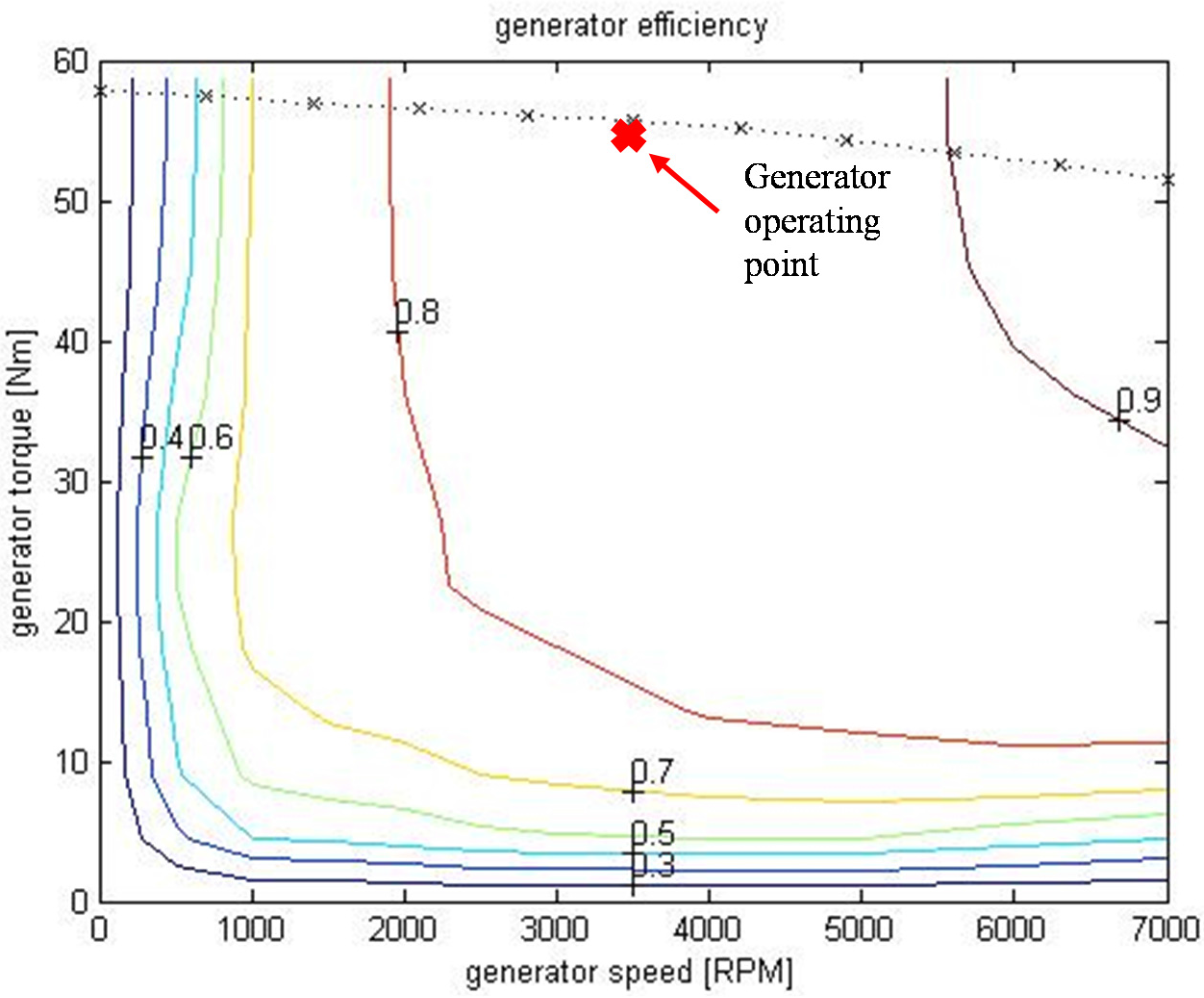
The generator model was used in only the SHEV system. In this model, a 32 kW permanent magnet generator is attached to a 1.0 L gasoline engine. The engine and generator are mainly controlled in a high-efficiency region during operation. The 1.0 L engine has high efficiency region around 3000 to 3500 rpm. The motor efficiency is also high (84% efficiency) in this region.
Figure 5 shows the operating point. Therefore, the engine speed and engine torque were maintained at 3500 rpm and 55 Nm, respectively, to obtain the optimal fuel economy.
Figure 5 shows the generator efficiency contour diagram. The data is retrieved from the ADVISOR 2003 database [
19].
Figure 5.
Efficiency contour diagram for the 32-kW generator.
Figure 5.
Efficiency contour diagram for the 32-kW generator.
2.4.3. Hydraulic Motor and Hydraulic Pump Models
In hydraulic plunger motor–pumps, plungers reciprocate in limited volumes, vacuuming low-pressure hydraulic oil into the plunger chamber and displacing high-pressure hydraulic oil outside the chamber through plunger compression. During this process, displacements can be regulated from pressure and flow rate variations by adjusting axial (clinoaxis plunger) or swashplate (swashplate plunger) angles, subsequently changing torsional moment and rotational speed relationships. The total efficiency of the hydraulic motor–pump is the product of volumetric and mechanical efficiencies. Operating variables such as pressure difference and volumetric flow rate, hydraulic motor–pump parameters (volumetric displacement), and fluid parameters (fluid viscosity coefficient, density, and bulk modulus) typically influence efficiency. The efficiency of the hydraulic pump and motor varies according to the operating conditions such as pressure and volumetric flow rate [
17]. The majority of the pump efficiency map, at a fixed flow rate, is populated with efficiency above 80%. Therefore, an overall efficiency of 80% was used for simulation. The hydraulic motor–pump-related equations are as follows:
The hydraulic motor/pump volumetric fluid flow rate is:
The hydraulic motor/pump shaft torque is:
The hydraulic motor/pump shaft power is:
where Q
PM is volumetric fluid flow rate;
xPM is the fraction of volume displacement;
DPM is the maximum volumetric displacement; ω
PM is the shaft angular velocity; ∆P
PM is the pressure difference between the hydraulic motor/pump outlet and the inlet; η
vPM is volumetric efficiency; η
tPM is mechanical efficiency; and
Z is mode factor (+1 for pumping mode, −1 for motor mode).
2.5. Energy Storage Component Model
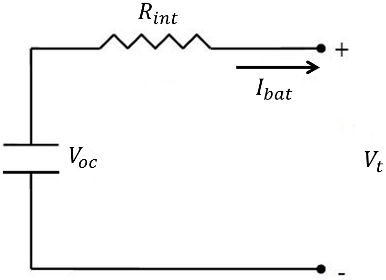
2.5.1. Lithium-Ion Battery Model
Lithium-ion batteries were adopted in this study. The total electric energy varied among PHEVs, SHEVs, and EVs, yielding 1, 2.5, and 25 kWh outputs, respectively. The battery model [
20] can be established according to the simple resistor–capacitor circuit shown in
Figure 6. The relevant equation is:
where
Voc is the open circuit voltage of battery;
Rint is the internal resistance of the battery;
Vt is the battery terminal voltage; and
Ibat is the battery output current.
Figure 6.
Resistor–capacitor circuit diagram for battery mode.
Figure 6.
Resistor–capacitor circuit diagram for battery mode.
After measuring terminal voltages and currents, the following equation is used to obtain the battery power outputs (
Pbat):
Furthermore, the following equation can be obtained by substituting Equation (9) into Equation (10):
Typically, battery SOCs are expressed using the battery capacity unit of amp-hour (Ah). Since SOCs vary by charge–discharge current, the following equation is used to obtain battery SOCs:
where
SOCint is the initial
SOC.
2.5.2. Accumulator Model
The energy that the accumulator requires from regenerative braking was calculated using the method proposed in [
21]. The equation E
k = 1/2 mv
2 was used to determine the energy of the accumulator. Assuming regenerative braking commences at
v = 60 km/h, 209 kJ of energy can be recycled during each regenerative braking event. Therefore, accumulator volume was set to 18 L, and working pressure was set to 172 to 344 bar. The accumulator model can be established according to the polytropic process of the laws of thermodynamics. The variation process of the gaseous state must be considered to investigate the gaseous pressures and volumes because the accumulator is operated frequently in the HHV. Therefore, the gaseous state changes were considered to be an adiabatic process (rapid changes;
n = 1.4) in this study. Temperature variations were not considered. During actual gaseous expansion and compression, the pressure and volume relationship is:
Oil displacements:
where
P0 is the initial enclosed gas pressure of accumulator;
P1 is the maximum actuation pressure;
P2 is the minimum actuation pressure;
V0 is the accumulator volume;
V1 is the volume with pressure
P1; an
V2 is the volume with pressure
P2; and
Vf is the volume of discharge oil from the accumulator.
Accumulator SOCs are typically expressed volumetrically because SOCs vary with volumetric flow rates. Therefore, the following equation can be used to obtain the accumulator SOC:
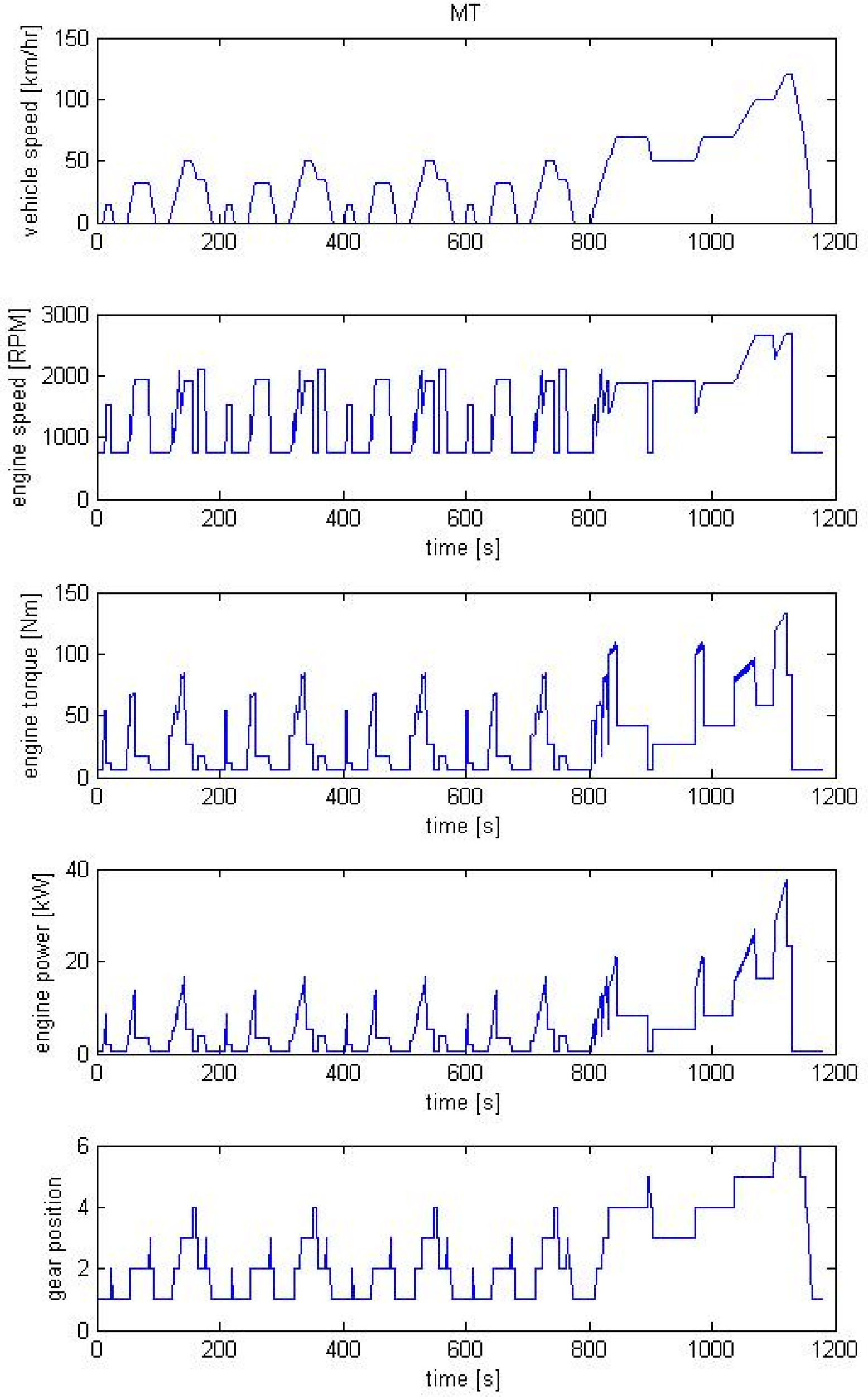
2.6. Manual Transmission Vehicle
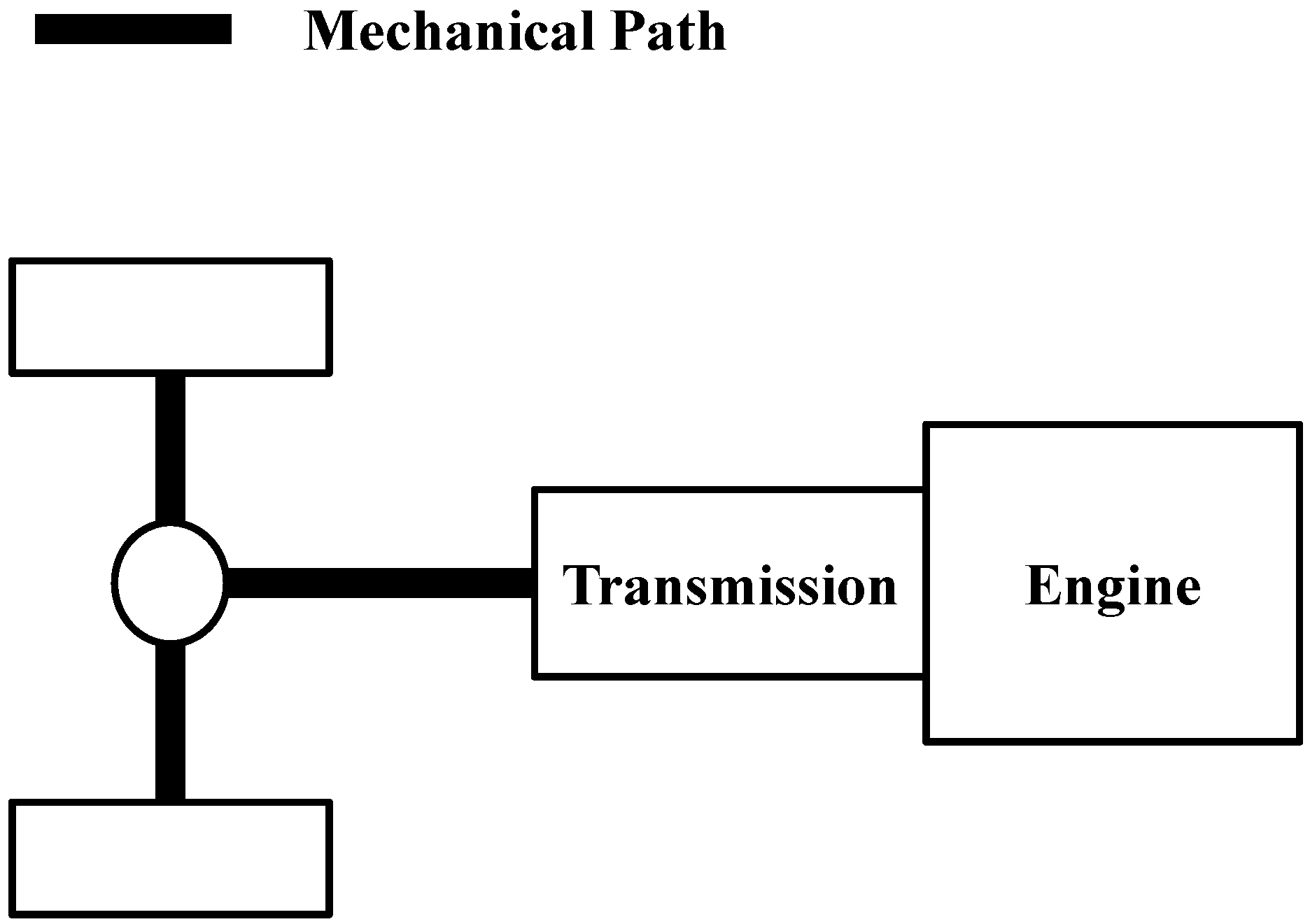
Figure 7 shows the conventional powertrain system model which comprised the subsystems of driving cycle, vehicle dynamic, transmission, and engine models. In the simulations, gearshifts were operated according to vehicle speeds and were assumed to be smooth and free from clutch slippage.
Figure 7.
Structural diagram of the manual transmission vehicle.
Figure 7.
Structural diagram of the manual transmission vehicle.
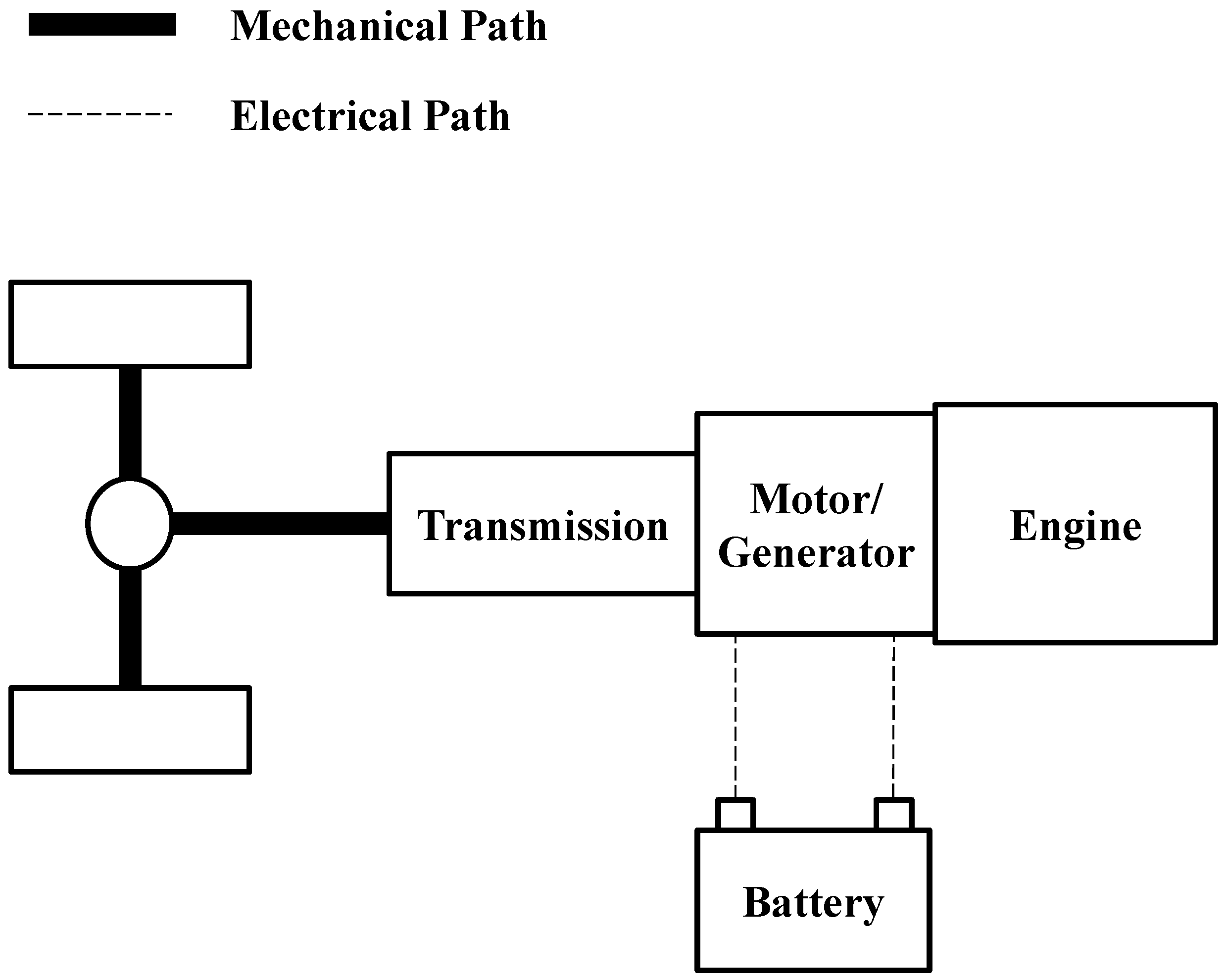
2.7. Series Hybrid Electric Vehicle
Figure 8 shows the SHEV powertrain system which comprised the driving cycle, vehicle dynamic, transmission system, power components (electric motor and generator), energy storage component (lithium-ion batteries), and engine model subsystems. In the simulations, the ON–OFF states of the engine were used to maintain the state-of-charge (SOC) of the lithium-ion batteries within a range of 0.35–0.65. The SOC range is designed to maintain the system in a high efficiency state, considering the combined efficiencies of both charging and discharging. The charging efficiency is high when SOC is low whereas the discharging efficiency is high when SOC is high [
22]. This study chose the middle 30% of SOC, 0.35 to 0.65. The control procedures involved inspecting the engine status, determining the SOC, and determining whether the engine must be switched on to charge the lithium-ion batteries.
Figure 8.
Structural diagram of the SHEV.
Figure 8.
Structural diagram of the SHEV.
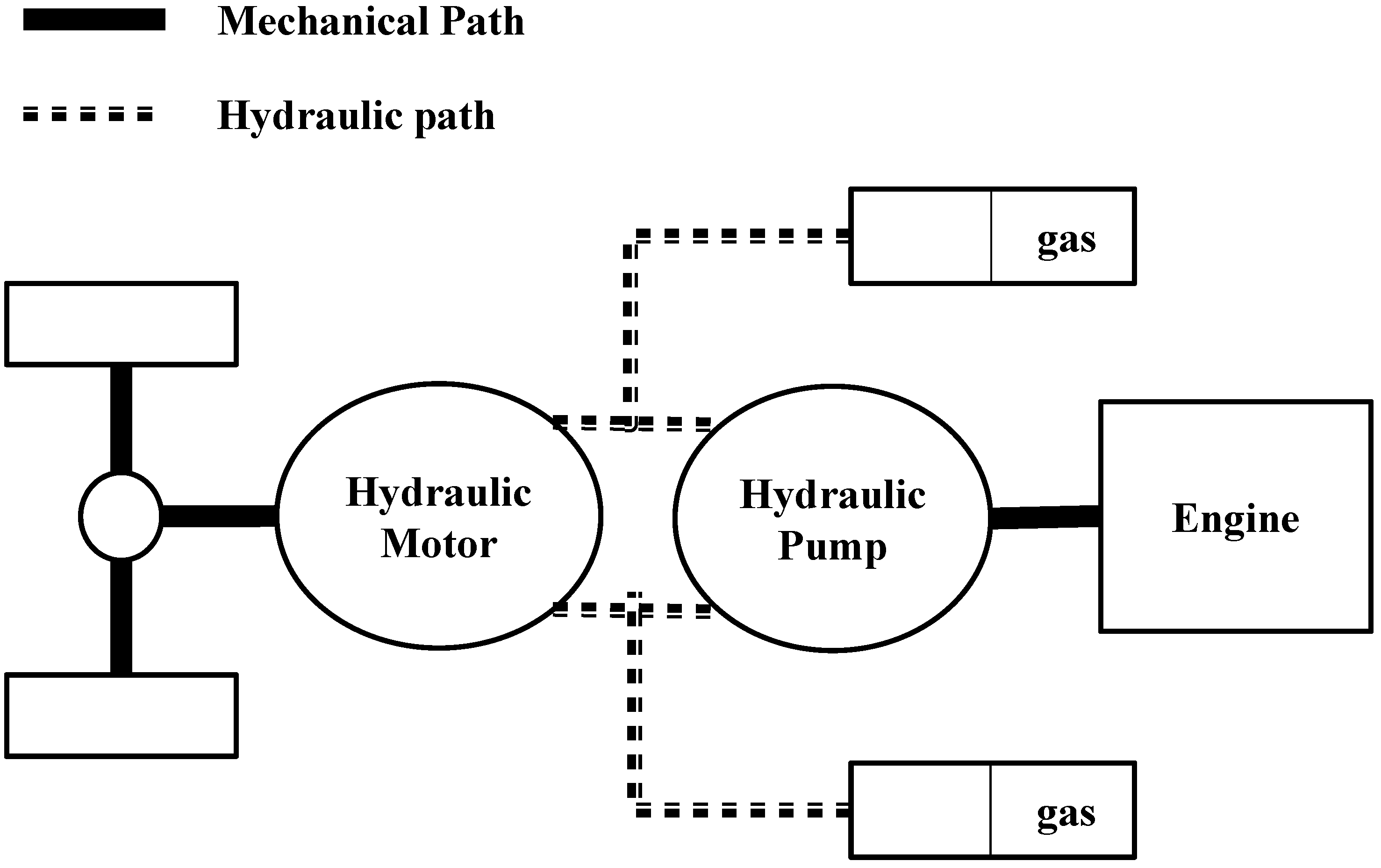
2.8. Series Hydraulic Hybrid Vehicle
Figure 9 shows the SHHV system model which comprised the driving cycle, vehicle dynamic, transmission system, power component (hydraulic motor and hydraulic pump), energy storage component (accumulator), and engine model subsystems. Regarding simulation controls, the ON–OFF states of the engine were used to control the SOC of the accumulator within the range of 0–1. The detailed control procedures were identical to those of the SHEV. The primary difference was that the accumulator had a larger SOC range than that of the lithium-ion batteries.
Figure 9.
Structural diagram of the SHHV.
Figure 9.
Structural diagram of the SHHV.
2.9. Parallel Hybrid Electric Vehicle
Figure 10 shows the PHEV system model which comprised the driving cycle, vehicle dynamics, transmission system, power component (electric motor), energy storage component (lithium-ion batteries), and engine model subsystems. Additionally, the simulation controls comprised pure electric (Mode A), pure engine (Mode B), hybrid (Mode C), engine charging (Mode D), and regenerative braking (Mode E) modes. In simulation, engine and electric motor torques were distributed according to specific road conditions (deciding among Modes A, B, and C) first. Then, the engine statuses were inspected to decide between the upper and lower SOC thresholds. The system proceeds to (engine) charging mode when battery SOC is below the set threshold; otherwise, the system proceeds according to the operating mode selected in the first step. The SOC operating range is maintained between 0.35 and 0.65.
Figure 10.
Structural diagram of the PHEV.
Figure 10.
Structural diagram of the PHEV.
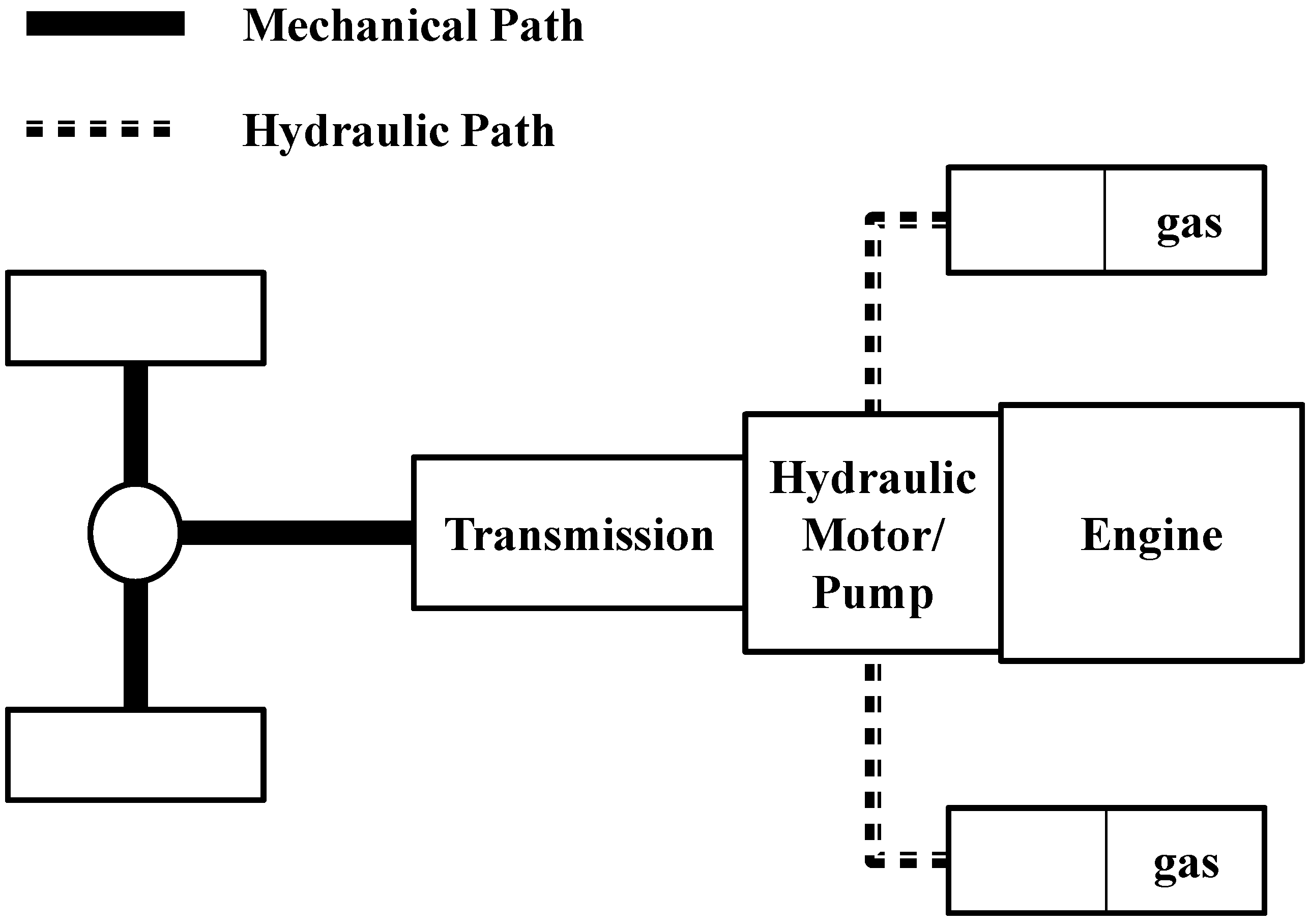
2.10. Parallel Hydraulic Hybrid Vehicle
Figure 11 shows the PHHV system which comprised the driving cycle, vehicle dynamic, transmission system, power component (hydraulic motor), energy storage component (accumulator), and engine model subsystems. The start–stop method was applied to improve fuel consumption during vehicle starting and stopping [
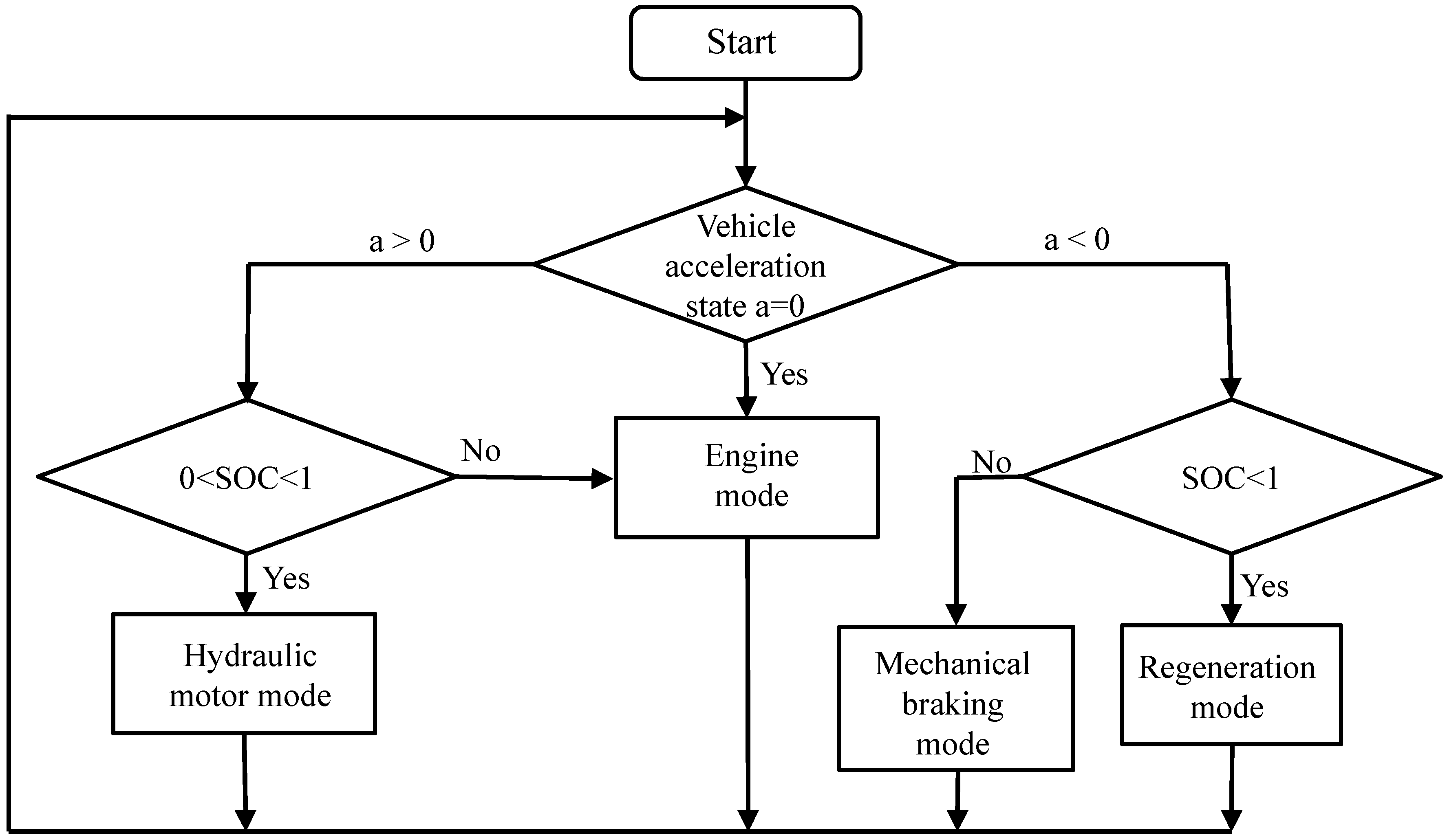
23]. The hydraulic motor and accumulator generated power for acceleration during vehicle startup. The vehicle was subsequently propelled by the engine as the accumulator depleted, and the engine was the only power source before the vehicle braking. The engine would be shut down when brake was applied. By preventing the engine from operating in an inefficient zone, this control strategy improves fuel economy. During vehicle braking, the hydraulic motor acts as a hydraulic pump that converts kinetic energy regenerated during braking into hydraulic energy and then recycles this energy to the accumulator for the next vehicle startup process. First, the state of vehicle acceleration was determined. When acceleration exceeds 0, the system proceeds to the second step to determine the SOC of the accumulator and to decide whether to operate with the hydraulic motor or in an engine mode. When acceleration equaled to 0, the system operates on engine mode, and when acceleration was less than 0, the system operates on regenerative braking mode,
Figure 12.
Figure 11.
PHHV structural diagram.
Figure 11.
PHHV structural diagram.
Figure 12.
PHHV control flow chart.
Figure 12.
PHHV control flow chart.
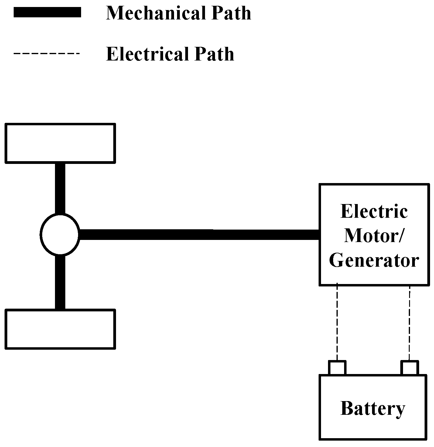
2.11. Electric Vehicle
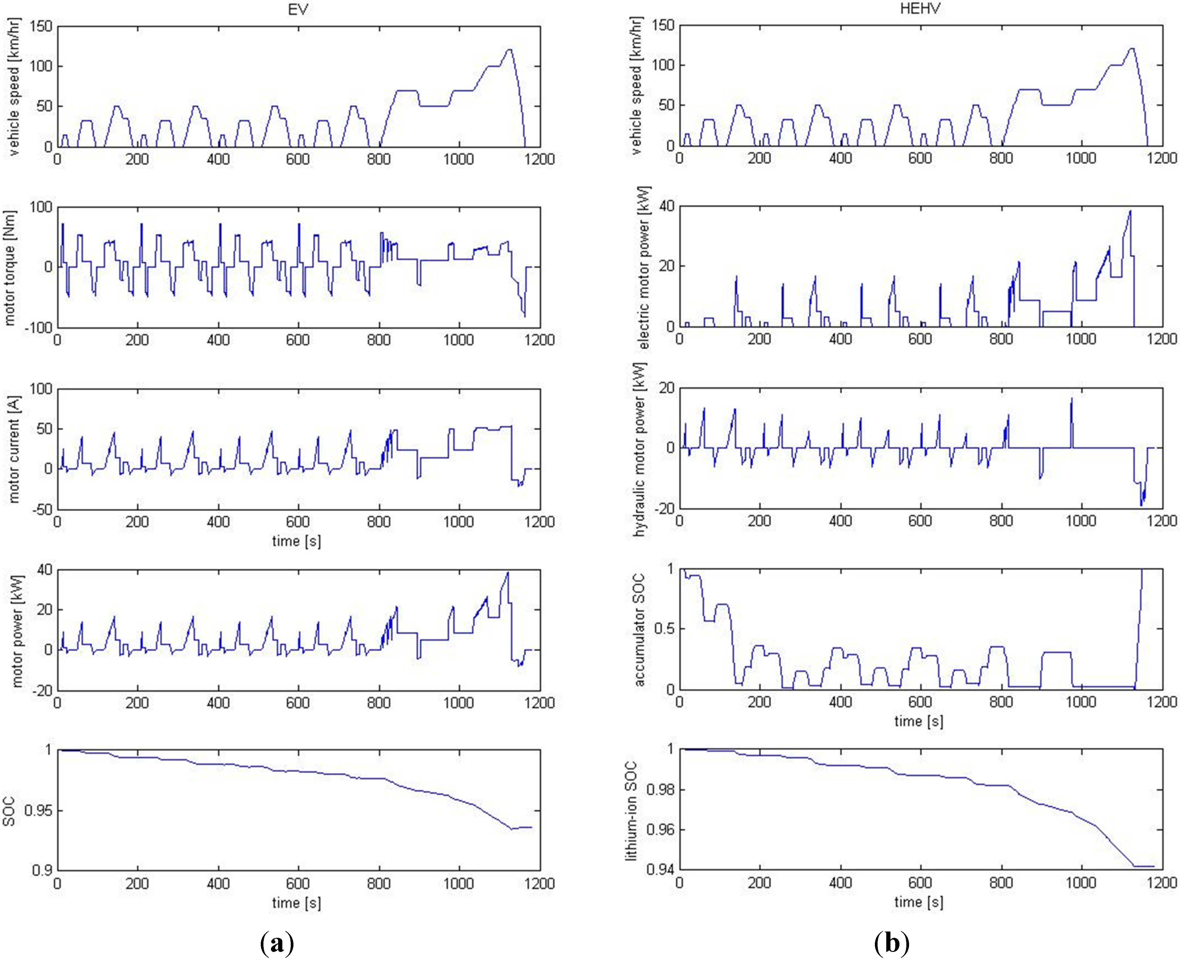
Figure 13 shows EV system which comprised the driving cycle, vehicle dynamics, transmission system, power component model (electric motor), and energy storage component (lithium-ion batteries) model subsystems. The simulations placed restrictions on the maximum motor speed, maximum motor torque, and maximum power of the electric motor. Additionally, the maximum and minimum voltages were configured for the batteries to ensure normal operation.
Figure 13.
Structural diagram of the EV.
Figure 13.
Structural diagram of the EV.
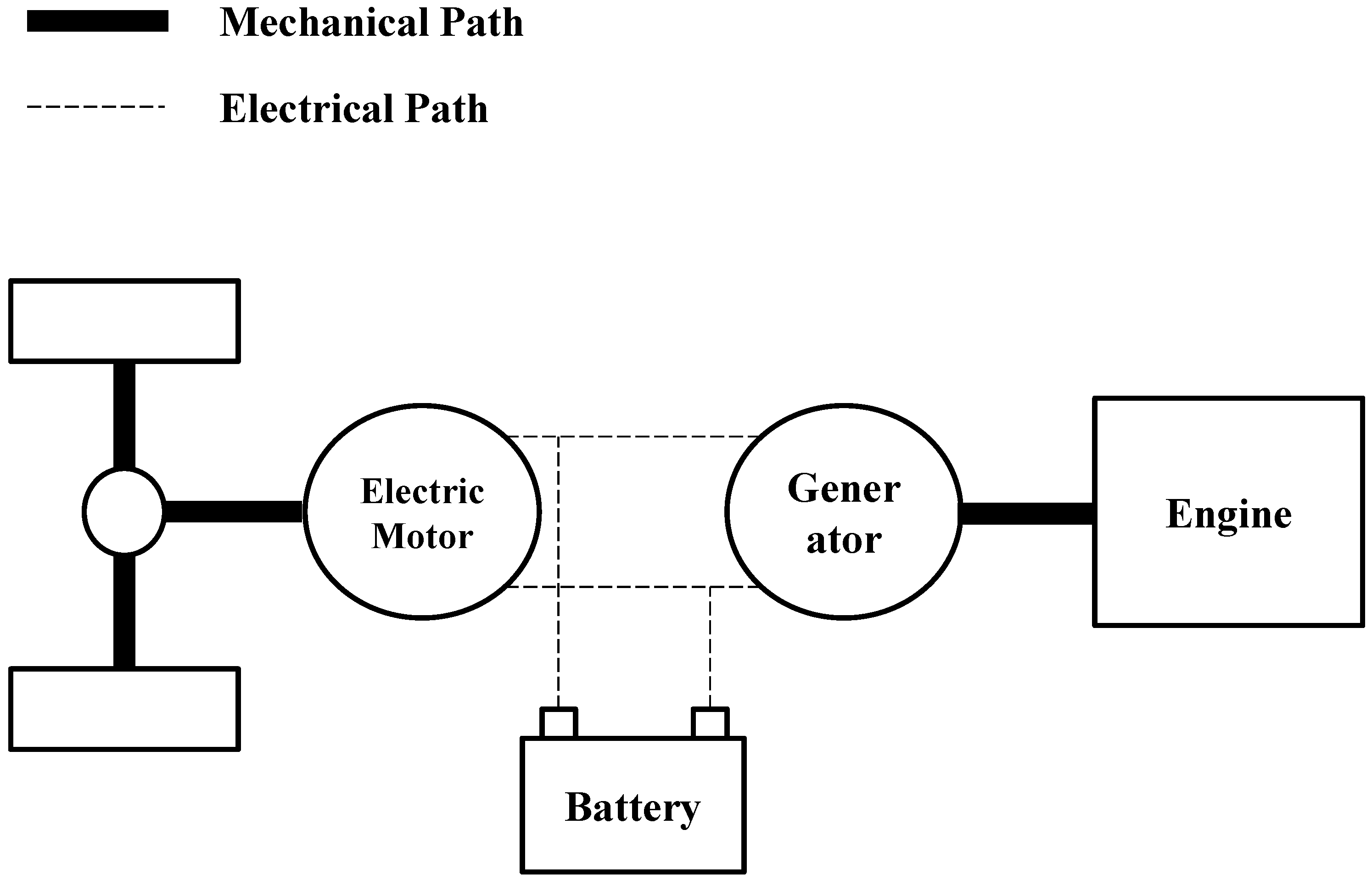
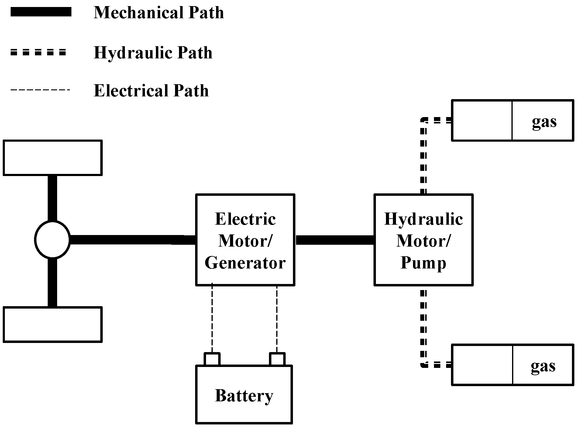
2.12. Hydraulic–Electric Hybrid Vehicle
HEHVs are primarily powered by electrical systems (electric motor and lithium-ion battery submodels) and assisted by hydraulic systems (hydraulic motor–pump and accumulator submodels). These systems reduce electrical energy consumption and extend the driving range (
Figure 14).
Figure 14.
Structural diagram of the HEHV.
Figure 14.
Structural diagram of the HEHV.
In simulations, the controls adopted the start–stop method identical to that applied in the PHHV system. In this study, the HEHV architecture was derived directly from that of the PHHV except the engine was replaced with an electric motor and battery. Therefore, the HEHV used the same control strategy as PHHV did, and the braking energy recycling was done by hydraulic motor instead of electric motor. The hydraulic motor is generally more efficient than the electric motor. In the HEHV, a hydraulic system is mainly used to recycle braking energy.
3. Simulation and Analysis
This section discusses the simulation results for the seven vehicle systems. Energy consumption was analyzed by simulating the NEDCs, and the performance of each component was compared. The required vehicle driving forces and powers for the NEDC were calculated first. Then, according to the performance analyzed for the manual transmission (MT) vehicles, the SHHV, PHHV, SHEV, PHEV, EV, and HEHV performance results were evaluated. Finally, the fuel economy of the SHHV, SHEV, PHHV, PHEV, EV, and HEHV systems was obtained.
3.1. Driving Force and Power Required for the Driving Cycles
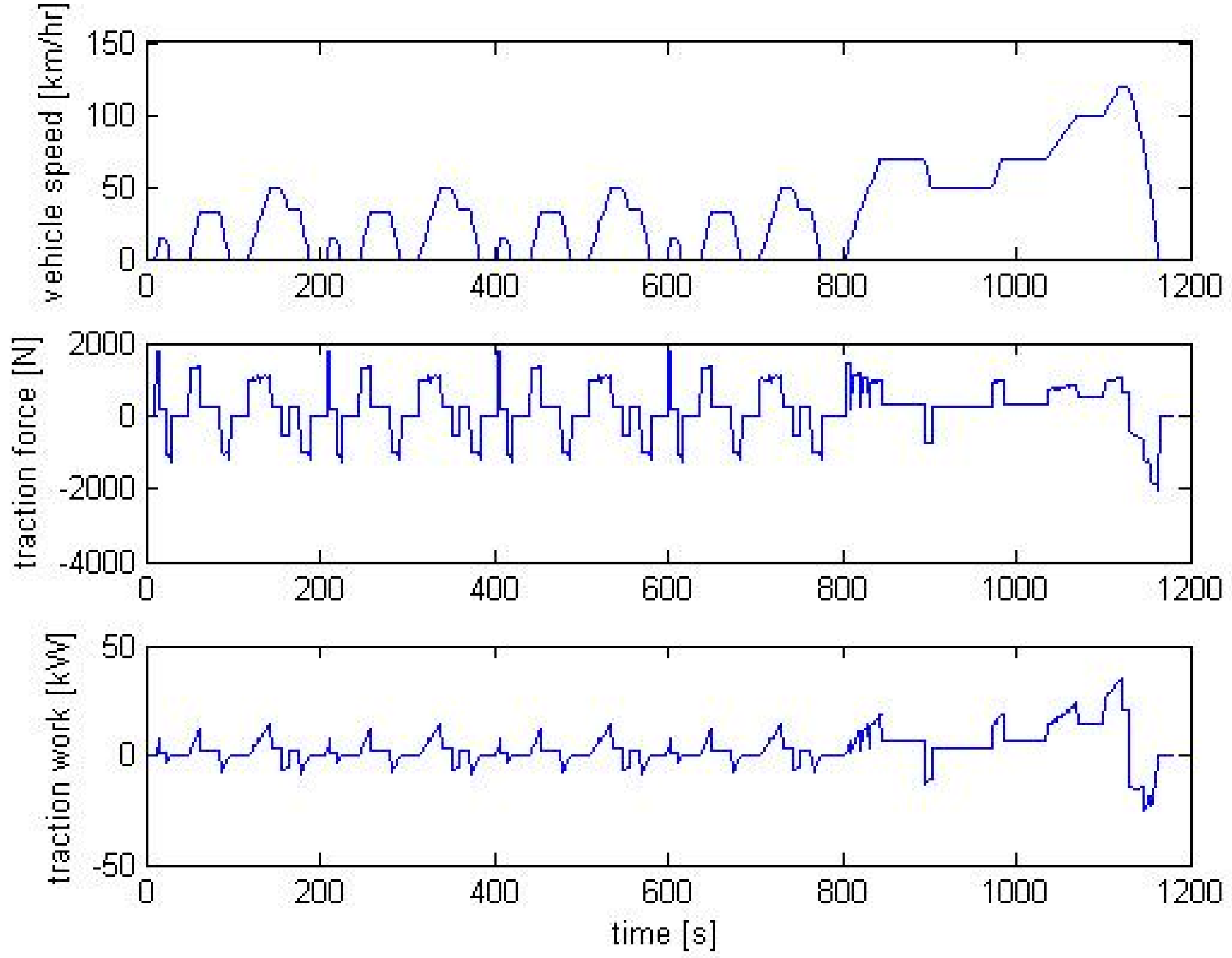
Regardless of vehicle type, specifications must be consistent in subsequent performance comparisons.
Table 2 shows the common vehicle specifications. For hybrid vehicles, the fuel economy is less sensitive to its vehicle mass since part of the kinematic energy used to accelerate the vehicle can be recovered by regenerative braking. Moreover, the study focused on the fuel efficiency of different powertrain configurations. To minimize the effects of different component masses, this study tentatively disregarded the mass differences of the vehicles in order to compare the actual functional contribution of different powertrain configurations. During simulations, the required wheel driving force and power must be calculated using the driving cycle model (
Figure 15). For example, the first, second, and third diagrams show the vehicle speeds, wheel driving force, and work required for the vehicles. The diagrams indicate that the maximal vehicle speed, wheel driving force, and power were 120 km/h, 1787 N, and 35 kW, respectively. Therefore, the power from the engine and electric motor in the series, parallel, and conventional vehicle systems should satisfy these conditions.
Table 2.
Common vehicle specifications.
Table 2.
Common vehicle specifications.
| Parameter | Symbol | Value | Unit |
|---|
| Vehicle mass | m | 1500 | kg |
| Frontal projected area | | 2.26 | |
| Air resistance coefficient | | 0.28 | — |
| Rolling resistance coefficient | | 0.008 | — |
| Wheel radius | r | 0.315 | m |
| Air density | | 1.225 | |
| Fuel density | | 0.74 | |
| Gravitational acceleration | g | 9.81 | |
Figure 15.
Vehicle speed, wheel driving force, and power.
Figure 15.
Vehicle speed, wheel driving force, and power.
3.6. Comparison of the Mass Effect on Energy Consumption
In all of the above simulations, vehicle mass was set to 1500 kg in order to focus on the energy efficiency of different powertrain systems. In this section, a 100 kg mass increment is added to the six derived powertrain systems to simulate the extra add-on masses from the energy storage medium, e.g., batteries and accumulators, and any energy transformation devices, e.g., motor/generators and pump/motors.
Table 8 summarizes the analytical results for the effect of mass on energy consumption, which indicate that, with extra mass increment, HEHV consume relatively less energy.
Table 8.
Mass effect on the per kilometer energy consumption.
Table 8.
Mass effect on the per kilometer energy consumption.
| kJ/km | m = 1500 kg | m = 1600 kg | Diff. |
|---|
| SHEV | 2174 | 2244 | 70 |
| SHHV | 1700 | 1793 | 93 |
| PHEV | 1586 | 1630 | 44 |
| PHHV | 1646 | 1707 | 61 |
| EV | 513 | 532 | 19 |
| HEHV | 455 | 469 | 15 |


