Earliest Deadline Control of a Group of Heat Pumps with a Single Energy Source

Abstract

In this paper, we develop and investigate the optimal control of a group of 104 heat pumps and a central Combined Heat and Power unit (CHP). The heat pumps supply space heating and domestic hot water to households. Each house has a buffer for domestic hot water and a floor heating system for space heating. Electricity for the heat pumps is generated by a central CHP unit, which also provides thermal energy to a district heating system. The paper reviews recent smart grid control approaches for central and distributed levels. An online algorithm is described based on the earliest deadline first theory that can be used on the aggregator level to control the CHP and to give signals to the heat pump controllers if they should start or should wait. The central controller requires only a limited amount of privacy-insensitive information from the heat pump controllers about their deadlines, which the heat pump controllers calculate for themselves by model predictions. In this way, a robust heat pump and CHP control is obtained, which is able to minimize energy demand and results in the desired thermal comfort for the households. The simulations demonstrate fast computation times due to minor computational and communication overheads.

1. Introduction

In northwestern European countries, approximately 40% of the entire energy consumption is for low temperature (less than 80 °C) heat, either for heating buildings or domestic hot water. The Netherlands relies for more than 90% of this demand on the combustion of natural gas in boilers. Although combustion of natural gas releases less carbon dioxide into the atmosphere than combustion of other fossil fuels, like oil and coal, recent agreements on limiting climate change necessitate a transition of existing heating system towards integration of renewable energy.

There are many ways to integrate renewable energy into existing supply-demand chains. One way is to replace natural gas by biogas. In Meppel, a new urban area is to be equipped with a hybrid energy system with a Combined Heat and Power unit (CHP) at the heart of the system for the production of heat and electricity. The heat is transferred into a district heating system, which is fed by multiple heat sources. The electricity is distributed to houses, each having a heat pump for space heating and domestic hot water [1].

Earlier, we investigated centralized control options for this hybrid energy system, focusing on the optimal control of the heat pumps with the objective to minimize peak electricity demand. This objective was chosen to enable balance between electricity production by the CHP and demand by the heat pumps. In [2], we investigate two control methods, one called global MILP (Mixed Integer Linear Program), the other called time-scale MILP, which solves the same problem with far less computational effort, but with equal quality of the solution. However, in [3], we further demonstrate how the control works within a model predictive control framework. With this framework, we demonstrate satisfactory thermal comfort. However, the optimization also steers towards frequent shifting of the heat pumps, which is problematic for the efficiency and lifetime of the heat pumps.

In this paper, we investigate possible solutions to improve the steadiness or robustness of the heat pump and CHP control. We investigate the applicability of possible solutions found in the literature to the original problem, i.e., central optimized control of a large group of heat pumps. The main contribution is the development of a control method based on earliest deadline theory and dynamic programming. We demonstrate that with this method, it is possible to reach near-optimum control strategies within a very short computational time with the desired robustness of the control of a large group of heat pumps and central CHP.

The paper is structured as follows. Section 2 discusses related work on robust control methods in relation to the linear program and algorithmic control of devices, like heat pumps and a CHP. Section 3 gives an overview of the methods we used for this paper, i.e., the simulation of house heat losses and the reference and ILP control method we used. We further explain the earliest deadline control framework. Results are shown in Section 4, and conclusions and future work are presented in Section 5.

2. Related Work

We first give an overview of smart control principles, which also serves as justification for the control method we propose. Smart grids, and specifically optimal control of devices like heat pumps or a CHP as part of a local renewable energy system, is a relatively recent investigation subject. The control of devices like heat pumps can be performed directly on a central or so-called aggregator level or on a distributed level (house or device level). The level on which devices are controlled determines the information that needs to be transferred between the aggregator level and the home or device level.

If the control is on the house level, each house may have a Home Energy Management System (HEMS), which plans the heat pump for itself. However, to reach a global objective for all heat pumps involved, the HEMS needs steering information from the aggregator level. As most applications of smart grids concern the public electricity network and involve smart control of numerous flexible devices, like washing machines, dishwashers and EV chargers, control on the distributed level receives most of the attention of researchers. In general, most Demand Side Management (DSM) methods aim at peak shaving of electricity flows on the transformer level. Methods for this include agent-based control, which uses the concept of price steering by auctions or dynamic pricing signals [4]. The work in [5] gives an overview of distributed control methods and combines auction-based control with predictions and planning methods as part of the Triana smart grid control framework. In practice, the concept of dynamic pricing may lead to the problem that devices may all jump to time intervals with the lowest price, thus increasing demand peaks in the future. This is improved by differentiated dynamic pricing [6]. A new control concept called profile steering was recently introduced in [7]. The work in [8] applies this concept for controlling a group of EV chargers, while [9] applies this concept to islanded operation of an electricity network, demonstrating positive effects on power quality within the entire network. Profile steering involves a planning phase based on predictions of consumption where each house is asked to plan devices, such that the house profile is as flat as possible. The aggregator then sums these profiles and compares the result with a desired grid profile. The deviations between the sum of the planned house profiles and the desired grid profile are used as steering signals during an iterative phase.

If the control is at the aggregator level, the aggregator decides which device will be switched on or off in time. The method we propose is that the aggregator defines a planning for the heat pumps and sends communication signals to the houses to start or stop the heat pumps. However, this planning may be overruled by a real-time control layer, e.g., a PID controller of a heat pump in case the planning leads to violations of certain operational margins, which may happen in case the prediction and, thus, the planning contain errors. The main advantage of directly controlling heat pumps from the aggregator level is that the home or device controllers may be simple or non-smart. The intelligence is on the aggregator level. The result is that each house needs to transfer information about the state of charge of a thermal storage, room temperature and status of the heat pump to the aggregator. The aggregator is then able to learn demand profiles from this information and to plan the heat pumps based on model predictive control principles. However, this type of information is privacy sensitive. Another possible disadvantage of this type of control is a reduced scalability towards large groups of heat pumps. Recently, clustering methods have been developed to reduce the complexity for large numbers of heat pumps and to increase scalability [10]. Another aspect to take into account is that direct control by the aggregator may not work not so well if there is much uncertainty to take into account. However, heat pumps operate in a predictable space heating or domestic hot water environment, with a low level of uncertainty. Hence, for a group of heat pumps that are owned by the same legal unit, like in the Meppel case, control on the aggregator level is an obvious choice. Like the heat pumps, the CHP is owned by the utility who operates the district heating network and a private electricity network, which is dedicated for supplying the heat pumps.

Not many authors investigate control on the aggregator level. Most authors remark on the problem of scalability [4,10,11]. However, in [2], we demonstrate the efficiency of a method called time scale linear programming, which involves prediction and planning, which is more accurate the closer the planning horizon is to the present time and less accurate for a planning horizon further into the future. In [3], we apply this method to a model predictive control simulation for a group of 100 heat pumps and investigate the quality of the obtained solutions. The algorithms show excellent results for the thermal comfort, which is subject to several constraints during the optimization. However, there are no constraints to limit the number of duty cycles of the heat pumps. As expected, this results in frequent on/off shifting of the heat pumps, which is not desirable for efficient operation and a long service life. An interesting question remains if a method can be developed other than defining more hard constraints on the heat pump operation cycles, which could limit the solution space considerably. In [12], the mathematical proof is given that minimizing peaks, which is typically the objective for the heat pump scheduling problem, is an NP-hard problem, which requires heuristics to solve. Fink develops an algorithm within a dynamic programming framework. The control algorithms presented in the present paper use a different approach and are based on the mathematical concept of Earliest Deadline First (EDF). A very readable introduction of EDF with the application of EDF in real-time task scheduling for embedded systems is given in [13]. This paper demonstrates the computational advantage of EDF, which we also show in the present paper. A similar framework to EDF called the color power algorithm is introduced in [14]. The suitability of this method for real-time DSM is demonstrated with a simulation of 100 electronic devices. However, in our case, a prediction and planning horizon is required due to the time delays of the thermal systems involved. As the planning horizon can be limited, EDF is suitable for (near) real-time control. Another advantage compared to other optimization methods used on the aggregator level is that predictions can now be made by the houses, and only their priority is communicated towards the aggregator level. This considerably relieves the privacy issues involved, but on the other hand, requires smartness on the device level.

3. Methods

3.1. Model Description

In our model, each house is equipped with a single heat pump that provides energy for heating the house and hot water for the domestic hot water demand. The electricity powering all heat pumps is generated by a single Combined Heat and Power unit (CHP) with the purpose to provide electricity only for these heat pumps with as little support from the electricity grid as possible. A schematic of the system is shown in Figure 1. The produced heat of the CHP is used to supply a district heating system, which contains a thermal storage for daily balancing purposes. We briefly consider proper sizing of this energy system. The number of houses with a heat pump determines the number of houses connected to the district heating system as follows. Let $D_{av}$ be an average daily thermal demand for a certain time period and $CO{P}_{av}$ the average heat pump coefficient of performance, i.e., the ratio between thermal production and electric power demand of the heat pump for that period. The daily produced electricity by the CHP is then $\frac{n·D_{av}}{CO{P}_{av}}$ with n being the number of houses with a heat pump. The district heating system uses the thermal production of the CHP. For this, the CHP can have a small size, just to produce the daily domestic hot water demand, or a larger size to produce also (part of) the demand for space heating. Let ${\eta }_e$ and ${\eta }_t$ be the electric and thermal efficiency of the CHP, respectively. Neglecting differences between the thermal demand of a house with a heat pump and a house connected to the district heating system and further neglecting district heating distribution losses, the minimum ratio between the number of houses connected to the district heating system (m) and houses with a heat pump (n) is then given by: $\frac{{\eta }_e·CO{P}_{av}}{{\eta }_t}$. Practical values for ${\eta }_e$, ${\eta }_t$ and $CO{P}_{av}$ are 0.4, 0.5 and 3.5, which yield the ratio: $\frac{m}{n}=2.8$. In our case there are 104 houses with a heat pump, which means that there should be more than 280 houses with a similar heat demand connected to the district heating system. In the Meppel case, more houses than that are projected, and the district heating supply system will also be supported by a wood boiler besides the CHP.

For simplification, we consider a discrete time model for the considered problem, meaning that we split the planning period into T time intervals of the same length. Furthermore, let H be the set of houses. In this paper, the index t denotes a time interval, and h denotes a house or a heat pump.

3.2. CHP Model

In [2,3], we presented how MILP can be applied to minimize peak electricity demand. This method is also used in this paper in the MILP control presented for comparison purposes. As our results in Section 4 show, MILP reduces the peak electricity demand. However, the aggregated electricity demand is changing very fast outside the peak demand periods, and any CHP is unable to react on such an unsteady electricity demand. Therefore, we replace the objective to minimize the peak electricity demand by a requirement that the aggregated electricity demand can be generated by the CHP.

The CHP in our model can operate in a few modes. In every mode, the CHP consumes some amount of gas and produces some amount of electricity and heat. In this paper, we study the electricity output. For every time interval, our algorithm chooses one mode in which the CHP will operate.

We pose the following objectives on the CHP control.

• The CHP should not switch the operation mode too often.
• Heat pumps should only consume the electricity generated by the CHP.
• The overproduction of electricity should be minimal.

Note that the electricity output generated by the CHP cannot be exactly equal to the aggregated demand of all heat pumps. Besides many technical reasons, which are not considered in our model, there is also the following mathematical one. For illustrative purposes, assume that the CHP generates 11 kW and that the electricity consumption of one heat pump is 2 kW. In this setting, we can either turn 5 heat pumps on and export 1 kW or turn 6 heat pumps on and import 1 kW. However, it is impossible to consume exactly the generated electricity. In our case study, exporting electricity is more preferable than importing. Therefore, our goal is to control the CHP and all heat pumps so that electricity is not imported and the export of electricity is smaller than the electricity demand of one heat pump. However, the control rules can be easily adopted if importing electricity is more preferable than exporting.

3.3. House Model

Every house is equipped with a heat pump that generates energy for heating the house and water for the Domestic Hot Water (DHW) demand. In order to model the heating demand of the house, we have developed in [3] a model predictive control approach based on an equivalent electrical circuit model representation of each house, consisting of two resistances and two capacitors. Model parameters are estimated by using data created by simulation in TRNSYS, which we explain in [15]. Other introductory papers on thermal network or electrical circuit models to predict building thermal energy demand are [16,17].

Each heat pump has only three modes: heating the house, heating DHW and off. Furthermore, to increase the efficiency of heating and the lifetime of the heat pump, we set the following constrains on the earliest deadline control of all heat pumps.

• The hot water buffer should be completely heated up every time a heat pump is turned to the hot water mode.
• A heat pump should not switch the operation mode too often. Therefore, a heat pump has to be turned off for at least m time intervals whenever it is switched off, and similarly, it has to heat the house for at least m time intervals whenever it is switched into the house heating mode. In the presented simulations, we consider two values of m: 4 and 8. These two simulations are abbreviated as ED4 and ED8.

In order to mathematically describe the control model of a house h, let $x_{h,t,SH}$ and $x_{h,t,CHP}$ be the binary variable, which denote whether the heat pump in a house h is heating the house (space heating) and DHW in time interval t, respectively. Since the heat pump cannot heat the house and DHW in the same interval, we require $x_{h,t,SH}+x_{h,t,CHP}\le 1$ in every time interval t and house h. The amount of energy injected into the space heating and DHW is $H_{h,SH}{x}_{h,t,SH}$ and $H_{h,DHW}{x}_{h,t,DHW}$ where $H_{h,SH}$ and $H_{h,DHW}$ are the heat output in space heating and DHW mode, respectively. The consumed electricity is $E_{h,SH}{x}_{h,t,SH}+E_{h,DHW}{x}_{h,t,DHW}$ where $E_{h,SH}$ and $E_{h,DHW}$ are the electricity consumption in space heating and DHW mode, respectively.

3.4. Demand Data

To study the quality of the control developed in this paper, we perform a simulation with 104 houses. For each house, the same equivalent electrical circuit model to calculate space heating demand is used, but with parameter differences between the houses, depending on the type of house. We also define schedules for occupancy-related thermal gains and losses, ventilation and domestic hot water consumption. The parameters, types of houses and schedules are explained in more detail in [3]. As we use the same models and input data for the model predictive control part and for the on-line simulation, we assume perfect predictions. Of course, this will be different in practice while weather forecasts are not perfect and occupancy-related schedules may vary substantially. This leaves an interesting question open for future work if this approach can be applied with sufficient accuracy in practice.

3.5. Control Algorithm

In order to control the CHP and all heat pumps, we developed an online algorithm based on the earliest deadline first technique. This algorithm has to decide operation modes of the CHP and all heat pumps for the coming time interval, which is denoted by $t_1$. This decision has two phases. First, an energy plan is computed by all house controllers and sent to the central controller. Second, these energy plans from all houses are used to determine the operation modes of the CHP and all heat pumps by the central controller. For this, the central controller needs from each house controller the following information:

• The possible electricity consumption of the heat pump in time interval $t_1$.
• $t_d$ the latest time interval (called deadline) when the heat pump needs to consume electricity.
• $l_{h,t}$ the lower bound and $u_{h,t}$ the upper bound for the total electricity consumption up to the time interval t. These two bounds follow from the fact that heating the house and the DHW can be shifted in time. Therefore, the upper (lower) bound is the maximal (minimal) amount of electricity that the heat pump can consume during the first t time intervals when the heat pump heats up as early (late) as possible.

3.6. Heat Pump Control

Both heating functions of the heat pump have some scheduling freedom, which determines the energy plan. The heat pump can consume electricity at time interval $t_1$ unless the heat pump was turned off less than m time intervals ago or both the house and the DHW buffer are fully heated up. Note that the deadline in the energy plan is not the earlier time of deadlines of the two heat pump functions because, e.g., when these two deadlines are the same, then the heat pump cannot fulfill both demands at once. There are various ways to calculate an energy plan, and we applied classical dynamic programming.

3.7. CHP Control

The CHP control has two parts. The first part determines the amount of electricity produced by the CHP, and the second one chooses which heat pumps will consume electricity in the time interval $t=1$. In the second part, all heat pumps are sorted by their deadlines, and the electricity is produced in this ordering until the CHP output is reached; see Algorithm 1.

Algorithm 1: Earliest deadline first rule.

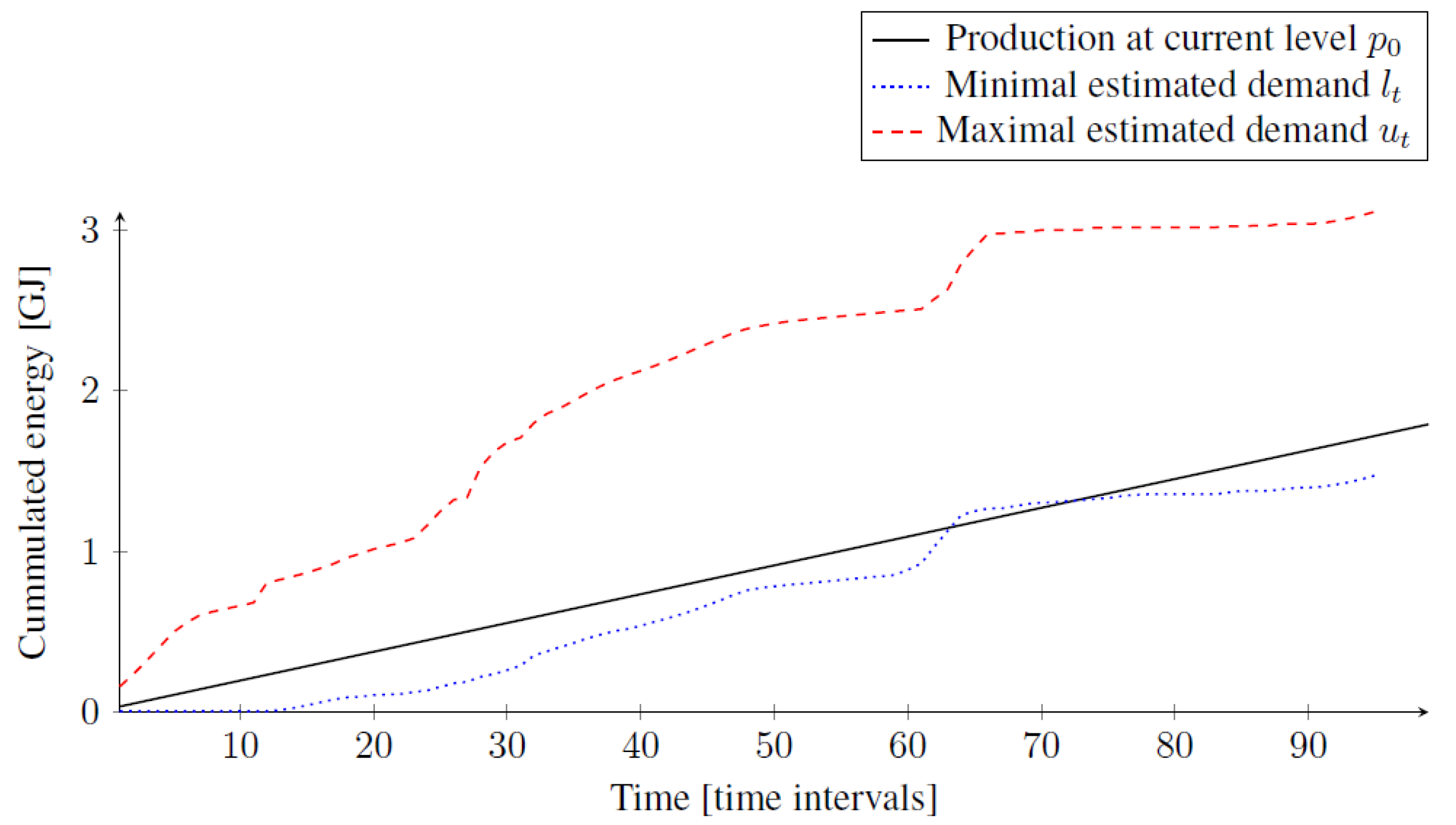
In order to determine the amount of electricity produced by the CHP, the aggregated lower $l_t={\sum }_{h\in H}{l}_{h,t}$ and upper $u_t={\sum }_{h\in H}{u}_{h,t}$ bounds are calculated. Figure 2, Figure 3, Figure 4 and Figure 5 show examples of such aggregated lower and upper bounds, and Algorithm 2 summaries the approach. Using these bounds, we can determine the production $p_t$ for time intervals $t\in T$, such that:

Algorithm 2: Algorithm deciding the operation mode of CHP.

• $l_t\le {\sum }_{i\le t}{p}_i\le u_t$ to ensure that the production up to the time interval t is between the minimal and the maximal demands and
• the number of time intervals $t\in T$ where the consecutive values $p_t$ and $p_{t+1}$ difference is minimal.

Note that the export of electricity in time interval t is $p_t-{\sum }_{h\in H}(E_{h,SH}{x}_{h,t,SH}+E_{h,DHW}{x}_{h,t,DHW})$.

However, since our algorithm is on-line, we only have to determine the production $p_1$ for the coming time interval $t=1$. Let $p_0$ be the power generated in the time interval $t=0$. In order to avoid frequent changes of the CHP mode, we keep the production $p_1$ on the previous value $p_0$ unless this choice leads to the underproduction or overproduction of electricity, for which we apply the following rules.

First, we find the minimal time interval $f\in T$ where the current production leads to underproduction ($l_f>f{p}_0$) or overproduction ($u_f<f{p}_0$). If there is no such time interval f in the planning horizon T, then we can safely keep the current production level. Otherwise, we continue by the following steps, which we describe only for the underproduction case, since the overproduction is similar. Figure 2 shows an example where energy output leads to underproduction at time interval $f=63$.

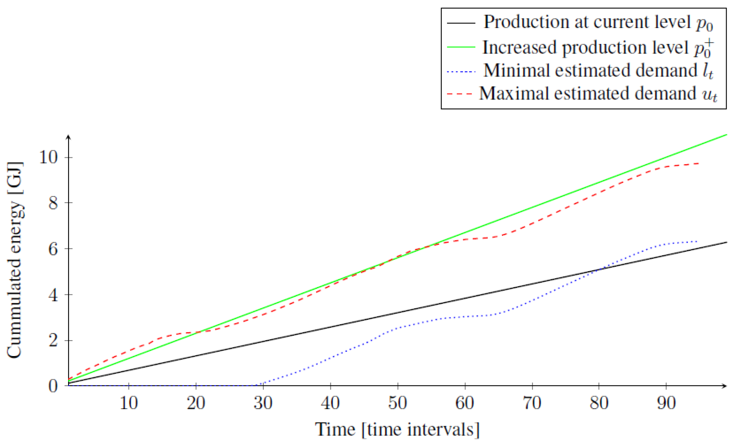
Second, let $p_0^{+}$ be the higher power output closest to $p_0$. If there exists time interval $t<f$, such that $u_t<t{p}_0^{+}$, then increasing the production level now leads to overproduction at the time interval t, so we keep the current production level $p_0$ at time interval $t=1$. This situation is presented in Figure 3, where keeping the current production level leads to underproduction at time interval $f=79$ and increasing the production leads to overproduction at time interval $t=19$, so it is better to keep the current production level. Otherwise, we again continue.

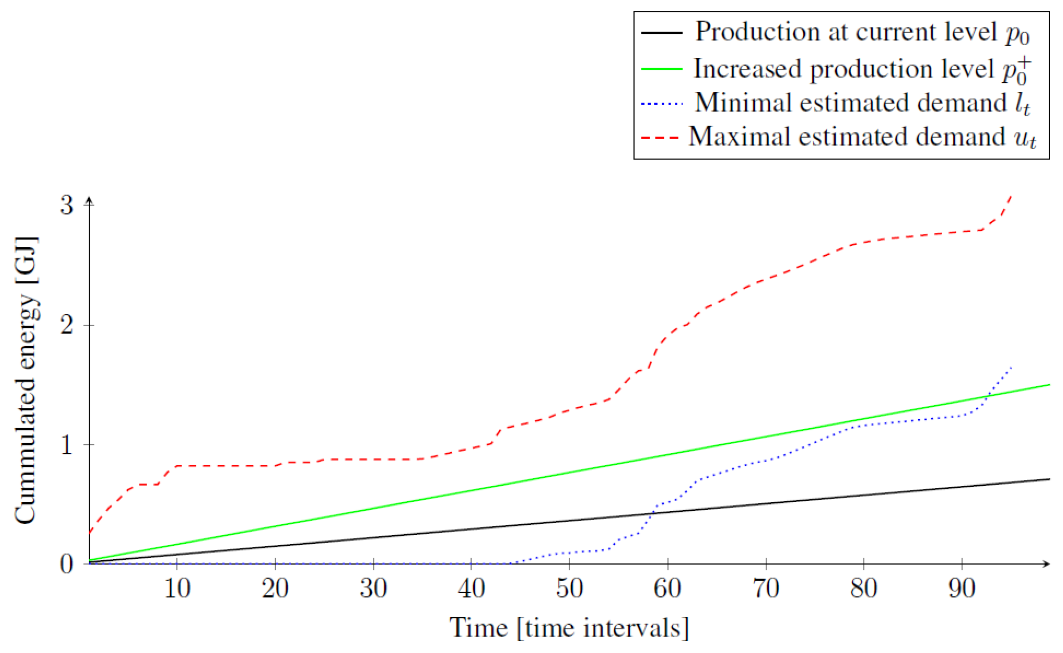
Third, we have to increase the production before time interval f, and the question is whether we increase it now or later. If we increase the production now, we may overproduce at some time interval, and we denote by a the smallest time interval, such that $u_a<a{p}_0^{+}$. However, if we increase the production in Time Interval 2, then a smaller amount of energy is produced, which may lead to underproduction, and we denote by b the smallest time interval, such that $l_b>p_0+(b-1)p_0^{+}$. If time interval b does not exist (that is, it is beyond the energy plan horizon T) or $a<b$, then we postpone increasing the production to avoid (or at least delay) the overproduction. This is presented in Figure 4, where the underproduction of the current production level occurs at time interval $f=58$. Overproduction of the increased production occurs at time interval $a=87$, while the time interval b is beyond the energy plan horizon. On the other hand, if the time interval a does not exist or $b<a$, then we increase the production now to avoid or delay the underproduction. See Figure 5 where the current production leads to underproduction at time interval $f=58$ and the increased production causes underproduction at time interval 93, so $b<93$ while a does not exist. If neither a nor b exist, we know that we have to increase the production before the time interval f, but there is no evidence proving that increasing the production now or later is better.

4. Results and Discussion

The simulation is performed for a whole year. In general, the heat demand is low during the summer months (only domestic hot water demand), increases towards the winter and peaks during several cold weeks during the winter. It is interesting to verify how the control behaves during the peak demand period and during periods with less space heating demand. The summer demand is from a control perspective much easier as each heat pump will operate until the fixed hot water thermal storage in each house is charged. For space heating, the control is somewhat similar, but this involves an adaptive storage size, depending on predictive energy balances. This part of the model predictive control for each house is explained in more detail in [3]. Therefore, we show results for two relevant weeks: a week with high heat demand during a cold winter period and a week with less heat demand in the spring season.

The control objectives for space heating are somewhat contradictory: the thermal comfort should be as close to desired setpoints as possible; the energy consumption should be as low as possible; and the number of times the heat pump switches on or off should be limited. We have shown in [3] that if the number of heat pump switches are not part of the control algorithm, optimal thermal comfort and minimal energy consumption is reached, but each heat pump switches rather frequently. Therefore, we implement an additional rule within the earliest deadline algorithm to keep the heat pump in space heating mode once it is turned on, for four up to eight consecutive time periods. With this, we investigate:

• if the number of times heat pumps switch on/off improved compared to MILP control. This is evaluated by counting the number of times the state of a heat pump changes (denoted by parameter $S{C}_{hp}$) and determining the average number of time intervals a heat pump operates for each of the two weeks (${\overline{OP}}_{hp}$).
• if the thermal comfort for each house is according to expectations. This is evaluated by summing for two categories (under and over temperature) the temperature difference between the achieved interior temperature and the set point interior temperature for each of the two weeks, divided by the total number of time intervals with under or over temperature, respectively ($\Delta T^{+}$ and $\Delta T^{-}$).
• if the CHP is controlled in such a way that it does not switch to different operation modes frequently. This is evaluated by counting the number of state changes of the CHP ($S{C}_{chp}$) for each of the two weeks.
• if the heat pumps are primarily supplied by the CHP, i.e., there is a minimal electricity flow to/from the grid. This is evaluated by summing the electricity flow to/from the grid, separated into under and over production and divided by the total number of time intervals with under or over production, respectively ($GRI{D}_{chp}^{+}$ and $GRI{D}_{chp}^{-}$); second, by determining the maximum flow for each of the two weeks ($MA{X}_{grid,chp}$).

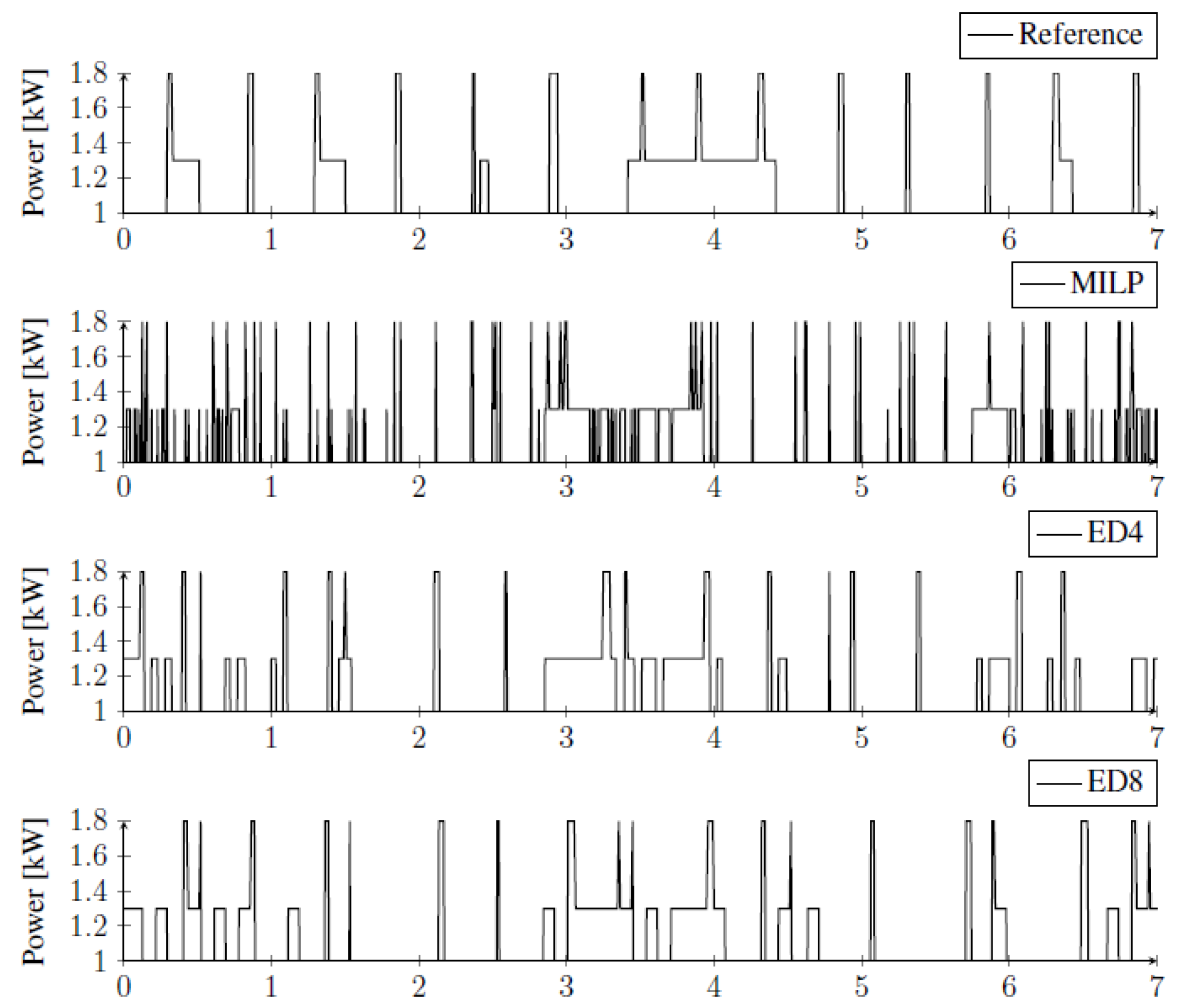
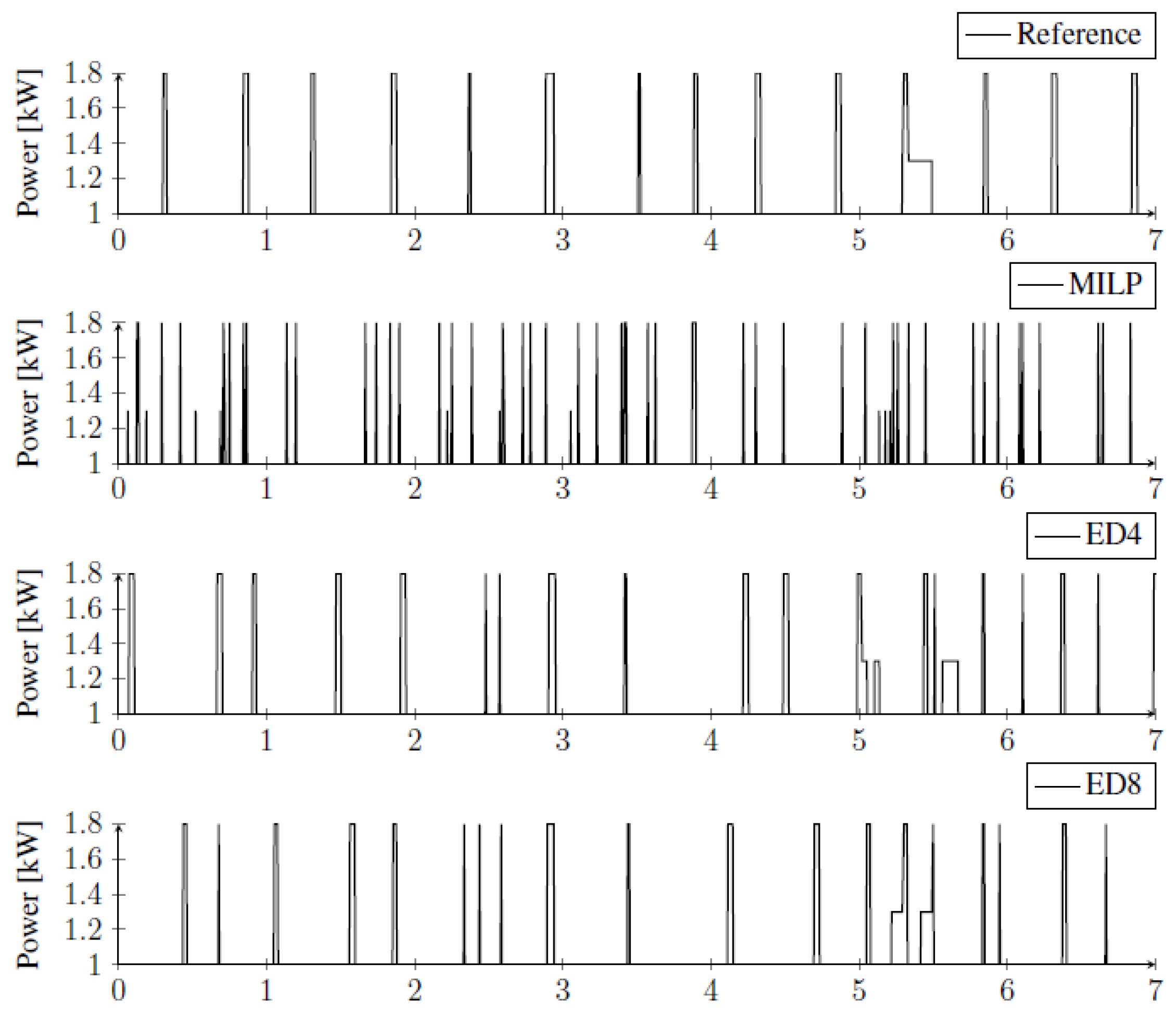
The robustness of the heat pump control can be investigated by evaluating the obtained switching behavior of every heat pump in time. There are no significant differences between the 104 heat pumps when it concerns the number of switches and the number of hours of continuous operation. The only significant difference is the moment when each heat pump starts and stops. Hence, it is sufficient to show only one example from the group of 104 heat pumps. For this, we choose the same case as in [3], i.e., a heat pump for a young family household. In Figure 6, the control of this heat pump is shown for the coldest week in the winter and in Figure 7 for the week in spring. In these figures, first the reference control is shown, which resembles conventional feedback control based on maintaining the room temperature within certain bounds around setpoint values and controlling the state of charge of the thermal storage. Second, the control obtained from MILP-algorithms presented in our previous work [3] is shown. Third, two cases of the control obtained from the ED-algorithms presented in this paper are shown. ED4 and ED8 signify the number of time intervals the heat pump is forced to be on (off) once it is turned on (off). ED8 has a larger size of a so-called space heating buffer than ED4, which leads to higher fluctuation of the interior temperature.

Results are summarized in

Table 1. Results. ED, Earliest Deadline.

Parameter	${\mathit{SC}}_{\mathit{hp}}$	${\overline{\mathit{OP}}}_{\mathit{hp}}$	$\mathbf{\Delta }{\mathit{T}}^{\mathbf{+}}$	$\mathbf{\Delta }{\mathit{T}}^{\mathbf{-}}$	${\mathit{SC}}_{\mathit{chp}}$	${\mathit{GRID}}_{\mathit{chp}}^{\mathbf{+}}$	${\mathit{GRID}}_{\mathit{chp}}^{\mathbf{-}}$	${\mathit{MAX}}_{\mathit{grid}\mathbf{,}\mathit{chp}}$
Unit	-	Intervals	°C	°C	-	kW	kW	kW
winter
reference	38	14.6	1.18	−1.11	386	-	-	-
MILP	200	2.5	1.72	−0.09	634	-	-	-
ED4	67	7.5	1.78	−0.10	30	0.99	0	39.3
ED8	58	10.5	1.92	−0.14	18	1.17	0	39
spring
ref	30	4.1	3.26	−0.24	297	-	-	-
MILP	112	1.1	3.34	−0.10	618	-	-	-
ED4	42	3.4	3.30	−0.04	13	0.69	0	1.7
ED8	40	3.3	3.40	−0.1	8	0.65	0	1.7

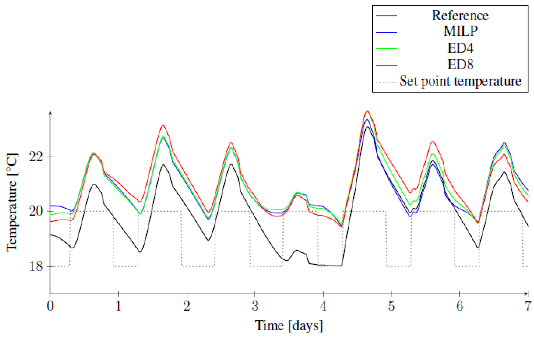
. For both weeks, ED control shows much less state changes of the heat pump ($S{C}_{hp}$) and longer time intervals of continuous operation (${\overline{OP}}_{hp}$) compared to MILP control. Notice also the difference between ED4 and ED8. The latter results are close to the number of state changes for reference control. However, heat pump control results should be discussed also in relation to the obtained room temperatures as a measure for the achieved thermal comfort and energy losses. The room temperatures are shown in Figure 8. Although reference control has the least heat pump shifts, the interior temperature is at some time intervals below the setpoint value. In Table 1, reference control has the largest values for $\Delta T^{-}$. Notice also an equally good performance of MILP control and ED control. We should indicate that the values shown for $\Delta T^{+}$ are of less concern. These slightly higher temperatures above the setpoints are caused by solar gains. During the heating season, slightly higher temperatures due to solar gains are usually not interpreted as comfort violations by inhabitants, and therefore, they are not cooled away.

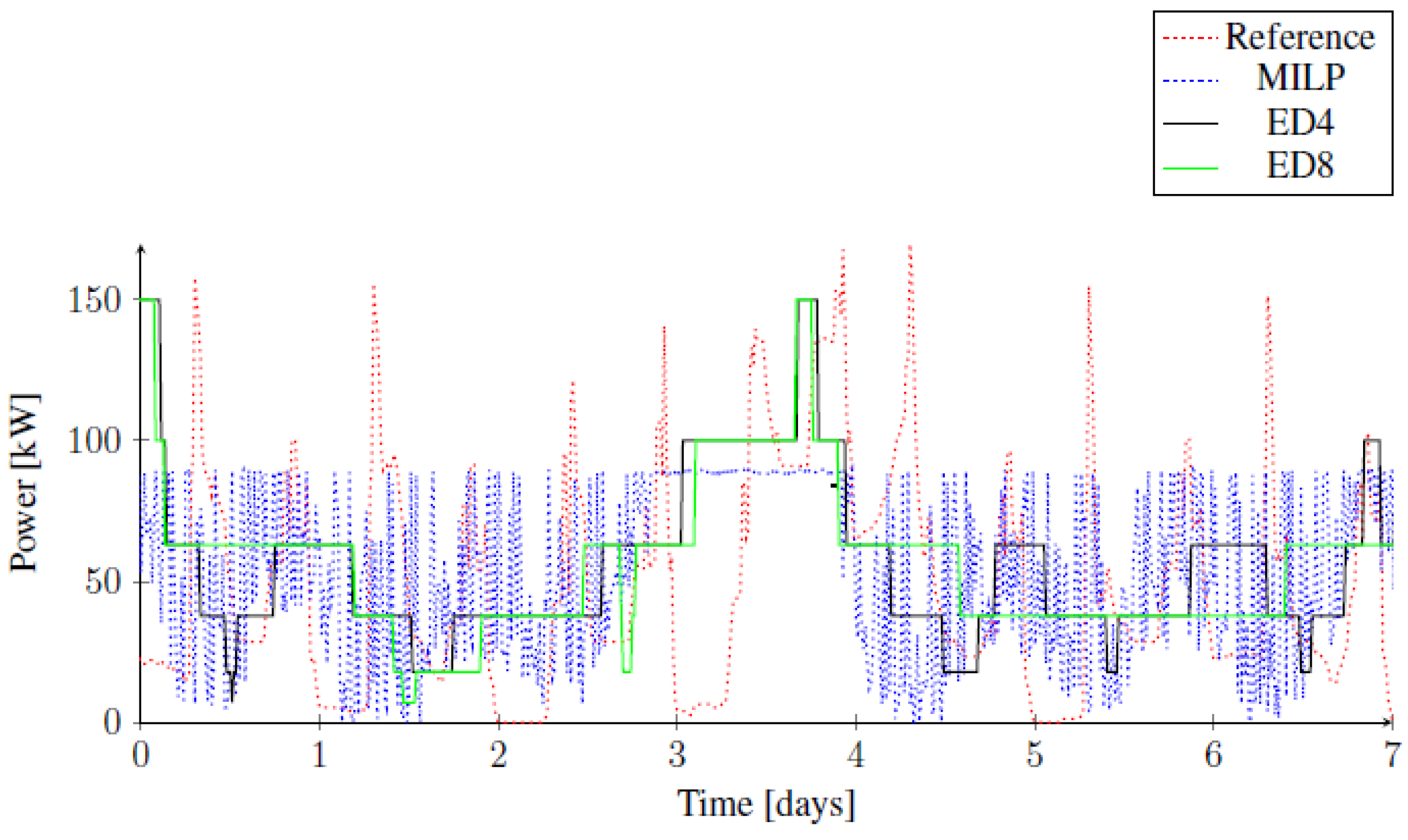
Control of the CHP is investigated for the same week in the winter and spring. Figure 9 shows the results for the week in winter, i.e., the reference control, MILP control and the two cases of ED control. Figure 10 shows the same for the week in spring. Results are also summarized in Table 1. Both figures demonstrate that the objective of the MILP control, i.e., to minimize the peak electricity demand is reached very well, but without additional constraints, this also results in a CHP control that changes the operational state of the CHP constantly; hence, the high values for $S{C}_{chp}$ in Table 1. The ED control shows very stable CHP operation, i.e., low values for $S{C}_{chp}$. However, ED control produces some peaks on the fourth day, i.e., the day with the highest heating demand, where most of the heat pumps simply have to run simultaneously and the CHP has to produce the associated electrical energy demand. On that day, the reference control is not able to support adequate thermal comfort (refer to Figure 8), and MILP control switches the heat pumps on and off the most frequently (refer to Figure 6).

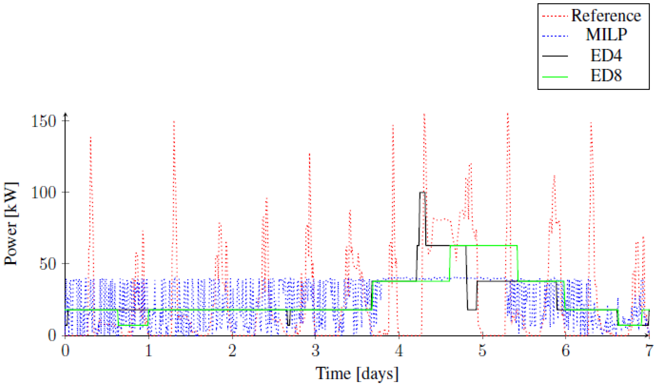
Figure 10 shows for the ED control an interesting advantage of the ED8 variant. In that week, on the fifth day, there is suddenly the first space heating demand of that week. Before that day, the CHP produces constantly the electric demand for some of the heat pumps to produce thermal energy for domestic hot water. On the fifth day, the ED8 variant produces a smaller peak than the ED4 variant. Therefore, the main advantage for the increased constraints on buffer capacity and operational time of ED8 is that this reduces the required production peaks of the CHP and may be an advantage for decreasing the size and costs of the CHP.

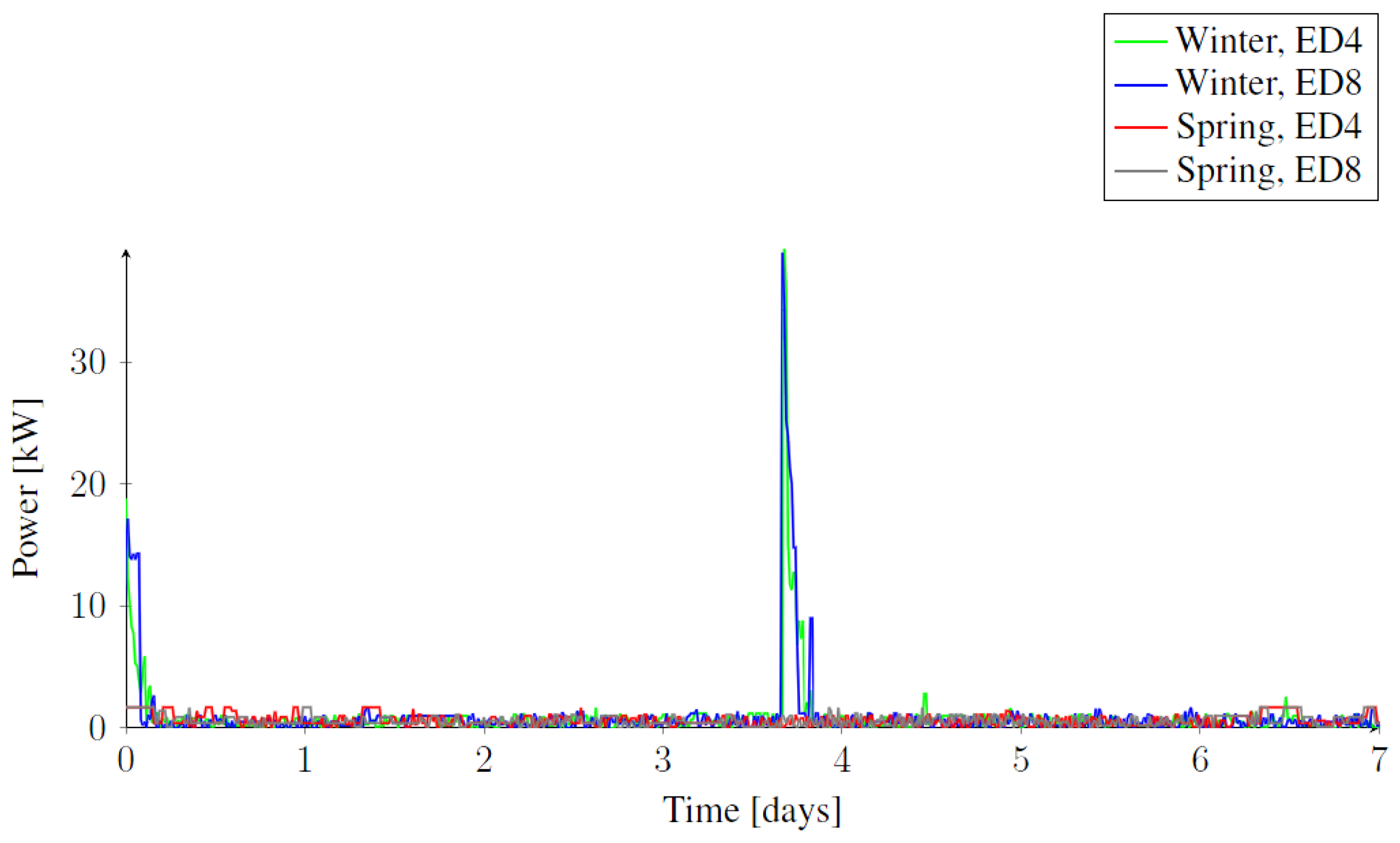
As explained in Section 3.5, ED control is programmed in such a way that the CHP is never producing insufficient amounts of electric energy for the aggregated demand of the heat pumps. Figure 11 shows that the CHP is always slightly overproducing, as is also seen in the value of $GRI{D}_{chp}^{-}$ in Table 1. In some intervals in the winter, when heat demand is the highest, the CHP has significant overproduction for short periods of time, seen from the peaks in Figure 11 and the value in winter for $MA{X}_{grid,chp}$ in Table 1. This is caused by the chosen control steps of the CHP and the programmed bandwidth between minimal and maximal estimated demand. If a larger range of steps is programmed and the bandwidth is narrowed, the overproduction peak is decreased and could vanish entirely. This is left as a matter of tuning the algorithms in practice.

For these simulation results, we use a computer with the processor Intel(R) Core(TM) i7-6700 CPU at 3.40 GHz using only a single thread. The running time of one simulation consisting of 104 houses and 1920 time intervals is 63 s, which is 315 $\mathsf{\mu }$s per one house and one time interval. Most of the running time is spent in the dynamic programming to determine the energy plan of each house at every time interval. It is possible to embed the house controller, such that it can run on a simple and inexpensive micro-controller. Furthermore, the amount of transmitted data between house controllers and the central controller is small. The energy plan sent from each house controller to the central one is made for a day (96 time intervals) ahead, so it consists of less than 200 numbers, which can be transmitted in a single TCP/IP packet. The response from the central controller is a Boolean for every house whether its heat pump is selected to run or not.

5. Conclusions

In this paper, we investigate the optimal control of a group of 104 heat pumps and a single Combined Heat and Power (CHP) unit, which is placed on the level of the aggregator. The heat pumps supply thermal energy for households for space heating and domestic hot water. Each house has floor heating for space heating and a thermal storage for domestic hot water. In previous work, we investigated the control of the heat pumps by Mixed Integer Linear Program (MILP) optimization and a faster algorithmic variant called time scale MILP, which makes central control of much larger groups of heat pumps possible. This results in the desired peak reduction of aggregated electricity demand of the heat pumps and thermal comfort for the households. However, the obtained control schemes of the heat pumps and CHP result in too much switching of these devices. Besides this, for privacy reasons, it is not desired to communicate household thermal comfort information towards a central controller. To overcome these problems, this paper presents an alternative control method based on the mathematical concept of Earliest Deadline first (ED). Unlike the previous mentioned methods based on MILP where all calculations were performed on the aggregator level, the houses now perform the model predictions of heat demand and communicate to the CHP their priority, which is done by specifying an upper and lower bound for the electricity demand up to a certain time interval. This relieves the previously-encountered privacy issues considerably.

Control results are shown for a cold week in winter and a warmer week in spring. Results for one heat pump are shown, as all heat pumps show similar results. The ED control method results in an equal thermal comfort for the households as the MILP control. However, the switching behavior of the ED heat pump control is now much better than the MILP control, which has an advantage for their operational life.

Similar to the heat pump control, the ED control of the CHP now demonstrates a very steady behavior of the CHP with only a few changes in the operational state of the CHP per week, contrary to the MILP control results, which showed many changes per day. The ED control also demonstrates peak reduction capabilities and the capability to choose if the CHP should always produce a bit less than, as close as possible to or more than the demand. This can be influenced by more sophisticated programming of the control states of the CHP, which is left for future work when this type of control is implemented in a real system. Furthermore, part of future work is to verify how the control behaves in practice and if a 15-min time interval for the evaluation of deadlines is sufficient. Another approach is to modify the earliest deadline rules so that the CHP and all heat pumps are controlled in real time.

Besides the advantages already mentioned, the ED-control algorithm appears to be very fast and is therefore ultimately scalable to larger and more complex energy systems. In the Meppel case, which is discussed in this paper, the heating system is separated from the domestic electricity supply system. However, in the future, the latter system may involve renewable energy from rooftop PV panels and smart control of flexible devices for each house, such as a battery charger/discharger and washing machine. The ED control may be extended to include this type of control, as well. In this way, depending on the application, ED-control may be an alternative to well-established smart grid control methods, such as cost-based or auction-based control. Part of future work is to further investigate to which extent ED control is capable of controlling more complex energy systems containing multiple energy supply sources and large numbers of flexible devices.