Dynamic Initial Weight Assignment for MaxSAT

Abstract

The Maximum Satisfiability (Maximum Satisfiability (MaxSAT)) approach is the choice, and perhaps the only one, to deal with most real-world problems as most of them are unsatisfiable. Thus, the search for a complete and consistent solution to a real-world problem is impractical due to computational and time constraints. As a result, MaxSAT problems and solving techniques are of exceptional interest in the domain of Satisfiability (Satisfiability (SAT)). Our research experimentally investigated the performance gains of extending the most recently developed SAT dynamic Initial Weight assignment technique (InitWeight) to handle the MaxSAT problems. Specifically, we first investigated the performance gains of dynamically assigning the initial weights in the Divide and Distribute Fixed Weights solver (DDFW+Initial Weight for Maximum Satisfiability (DDFW+InitMaxSAT)) over Divide and Distribute Fixed Weights solver (DDFW) when applied to solve a wide range of well-known unweighted MaxSAT problems obtained from DIMACS. Secondly, we compared DDFW+InitMaxSAT’s performance against three known state-of-the-art SAT solving techniques: YalSAT, ProbSAT, and Sparrow. We showed that the assignment of dynamic initial weights increased the performance of DDFW+InitMaxSAT against DDFW by an order of magnitude on the majority of problems and performed similarly otherwise. Furthermore, we showed that the performance of DDFW+InitMaxSAT was superior to the other state-of-the-art algorithms. Eventually, we showed that the InitWeight technique could be extended to handling partial MaxSAT with minor modifications.

1. Introduction

Maximum Satisfiability (MaxSAT) is a general optimization NP-hard [1] form of the well-known NP-complete propositional Satisfiability (SAT) [2]. Given a propositional SAT encoded problem in Conjunctive Normal Form (CNF), where CNF consists of a set of conjunctive clauses and each clause consists of a set of disjunctive literals (propositional variables) or their negations, a solution to a MaxSAT problem is the one with the maximum number of satisfied clauses. One important role that makes MaxSAT of particular interest within the SAT community is that a solution is accepted with some optimality level. Thus, handling real-world problems by employing MaxSAT methods is more practical, as many, if not most, real-world problems are unsatisfiable (an assignment that satisfies all the clauses does not exist). As a matter of fact, in [3], the Local Search (Local Search (LS)) solving techniques were mainly designed to handle the MaxSAT problems. Then, the techniques were extended to solve the SAT problems as in [4]. Therefore, instead of searching for a completely optimal solution, MaxSAT solving methods aim to find the assignments with the maximum number of satisfied clauses. MaxSAT has many applications in real-world problems such as planning, timetabling, scheduling, bioinformatics, and intelligent routing, which are imperative in artificial intelligence or its related fields. Therefore, MaxSAT is of exceptional interest to researchers in the SAT community, as finding a general-purpose solver that could find near-optimum solutions to MaxSAT is an open research area with significant potentials.

In the literature, there are two main tracks for handling MaxSAT problems: (1) the complete track (also known as the systematic or exhaustive track) such as EvalMaxSAT [5] (which was implemented in the MSCGMaxSAT solver [6]), such as RC2, the winner of the unweighted and weighted main track MaxSAT evaluation in 2018 [7], or (2) the incomplete track, such as Stochastic Local Search (Stochastic Local Search (SLS)) like tabu search [8,9], simulated annealing, scatter search [10], evolutionary algorithms [11], dynamic local search [12,13,14,15], and hybrid SLS [16,17].

While both tracks, complete and incomplete, share the same goal of finding a solution for the MaxSAT problem, they differ widely on how to achieve this goal. The complete track algorithms exhaustively search the problem space. Therefore, a conclusion is drawn about whether the problem has an optimum solution if one exists. Unlike complete algorithms, the SLS algorithms explore the search space stochastically until they discover a good solution within the time constraints. Therefore, they are faster at finding a solution and incur less computational cost. However, they compromise on finding an optimum solution and cannot conclude that a good solution does not exist.

On the one hand, the tradeoff incurred by the search completeness is that it is computationally costly when applied to solving large problems where it struggles with the computational resources and meeting the time constraints. However, the complete search algorithms can guarantee finding an optimal solution if one exists. On the other hand, the incomplete attribute of Track 2 led to the fact that the SLS algorithms can handle large problems and find good (near-optimum solutions) in relatively acceptable computational cost and time constraints with the expense of reaching optimality.

SLS solvers belong to a family of techniques known as metaheuristic methods, where the solvers are either global search-based or Local Search-based techniques (LS). In general, global-based search is derived from and mainly inspired by natural design. For example, Ant Colony Optimization (Ant Colony Optimization (ACO)) is a known algorithm to handle SAT optimization problems [18], which is inspired by ants while searching for food (which involves keeping track of the colony and finding the best paths to a food source. Another example is the Genetic Algorithms (Genetic Algorithm (GAs)), where they globally use stored data generated in the search process’s past stages. The data are then used to inform the search process better and guide the search toward more promising areas within the search space. Genetic algorithms were mainly inspired by Darwin’s theory of the natural selection process, where chromosomes store past data, and the data are utilized to make future relatively better decisions. Another interesting naturally inspired global-based searching method is Swarm Intelligence (SI), which recently has been shown to be efficient in handling optimization problems and real-world industrial problems such as scheduling [19,20] and vehicle routing [21].

Local Search (LS) differs from global search metaheuristics where LS, instead of relying on global changes to be made within the search space, depends on information gathered from local neighboring areas of the search’s current stage. Otherwise, the local search and global search metaheuristics target the same goal, where a solution to an SAT problem is accepted with some level of goodness rather than an optimum one. They also share the characteristics of the incompleteness of searching for a solution (where they do not fully explore the search space).

MaxSAT has been studied for decades and exhaustively investigated. As a result: (1) advances in handling MaxSAT and its solving technologies and algorithms have been proposed; (2) the MaxSAT problems have been generally categorized into three primary forms: unweighted MaxSAT, Partial MaxSAT, and weighted MaxSAT. Unweighted MaxSAT is a problem that makes no distinctions about the importance or hardness of the constraint. For instance, in a CNF MaxSAT-based encoded problem, the cost of flipping a variable (changing its Boolean value from true to false or vice versa) is counted based on all clauses’ exact cost functions. The other and more general form of MaxSAT is Partial MaxSAT (Partial Maximum Satisfiability (PMS)), where the clauses are divided into two types: hard clauses and soft clauses. An accepted solution to PMS must satisfy all the hard clauses and a maximum number of soft clauses. The third form of MaxSAT is Weighted Partial MaxSAT (Weighted Partial Maximum Satisfiability (WPMS)), where each soft clause has an associated unit of weight.

Since the development of the well-known LS techniques, GSAT+weight, and the breakout method in 1993 [22,23] that uses weights (penalties) to alter the search space to escape from traps (local optimum), a branch of LS known as Dynamic Local Search (Dynamic Local Search (DLS)) was developed. DLS algorithms have been among the best performing solving algorithms on randomly generated problems as per the SAT competition results (as in http://www.satcompetition.org (accessed on 20 March 2021)) for almost a decade.

Our Contribution

Based on the above discussion and given the importance of the MaxSAT problem, our focus in this research was to study possible approaches to developing and/or enhancing the current state-of-the-art DLS algorithms for unweighted MaxSAT. More specifically, the main contributions of this research focused on:

• Investigating mechanisms that have a general effect or improve the current state-of-the-art MaxSAT solving mechanisms, as they successfully deal with real-world problems with huge sizes and variables exceeding millions in number, which a decade ago was not possible
• We were interested specifically in experimentally investigating whether employing the dynamic initial weight allocation [24] within the SAT solvers had a widespread impact on the performance of algorithms that handle MaxSAT problems. We were further interested in testing whether this impact reflected negatively on the solver’s performance or led to a higher performance level
• Based on the above two points, we designed the paper to address unweighted MaxSAT problems because the transition to weighted partial MaxSAT problems is implicit and requires only some very minor changes. Consequently, we experimentally investigated the dynamic initial assignment implemented in the DDFW+Initial Weight assignment technique (InitWeight) [24] and compared it against the state-of-the-art algorithms: YalSAT [25], ProbSAT [26], Sparrow [27], and DDFW [28]. These algorithms are generally applied to solve SAT problems; therefore, they are particularly suited to our purpose to extend and investigate the performance of the dynamic initial weight assignment in handling MaxSAT, where we adjusted the solvers to preserve and store the solutions that were reached and the time within which those solutions were reached.

In the next Section 2, we discuss the preliminaries used in the paper. In Section 3, we discuss a general overview of the dynamic local search approaches. Then, in Section 4, we illustrate the improvement gains by our approach, and then, we analyze the results. Finally, the conclusion is drawn in Section 5.

2. Preliminaries

We considered the SAT formula ($\mathcal{F}$) encoded in Conjunctive Normal Form (CNF), which consists of a conjunction (⋀) of Clauses (Clause (Cl)) where each clause consists of disjunctions (⋁) of Literals (Literal (Lit)). A literal $\left(Li{t}_i\right)$ is a propositional variable whose value is either true or false. A variable or its negation could occur in some clauses. For example, given two clauses, Clause 1 ($C{l}_1$) and Clause 2 ($C{l}_2$), variable X may occur in $C{l}_1$ as in $(x\vee y\vee z)$ and occur in $C{l}_2$$(x\vee a\vee \neg z)$. We denote that Clauses 1 and 2 are neighbors as variable X$\in (C{l}_1,C{l}_2)$ because they share the same signed literal x of variable X. Given a third clause $C{l}_3$$(a\vee b\vee \neg z)$, the clauses $C{l}_1$ and $C{l}_3$ are not neighbors as the variable Z occurs in both clauses with different literal signs. A solution to the MaxSAT formula ($\mathcal{F}$) is an assignment that satisfies a maximum number of clauses in $\mathcal{F}$. A clause $C{l}_i$ is satisfied if ∃$Li{t}_{C}li$ = true $\in C{l}_i$. The cost function $cost\left(\mathcal{F}\right)$ denotes the number of satisfied clauses at any given stage during the search, and we denote $bestCost\left(\mathcal{F}\right)$ as the maximum number of satisfied clauses reached by a given assignment during the search (or the minimum number of unsatisfied clauses reached). We also denote the time at which $bestCost\left(\mathcal{F}\right)$ is reached by $time\left(bestCost\right)$.

Furthermore, as our study crucially depended on the general problems’ structure, we denote the following:

• TotalnumberofClauses(nCls): the total number of clauses within the formula $\mathcal{F}$.
• AverageNeighborhoodSize(AvgNeighbS): the average of the clauses’ neighborhood size. For each problem set, the sum of literal occurrences for each clause is divided over the total number of the clauses in $\mathcal{F}$:

  $$AvgNeighbS=\frac{{\displaystyle \sum _{i=1}^{nCl}Lit\_Occurrences\left(C{l}_i\right)}}{nCl}$$

  (1)
• SolutionCost(SolCost)$\left(\mathcal{F}\right)=$ the total number of unsatisfied clauses in the current assignment.
• MoveCost(MoveCost)$=$ the difference of the number of clauses that will become unsatisfied and the number of clauses that will become satisfied by flipping a literal from true to false or vice versa.

  $$\mathit{AverageClauseSize}\left(\mathit{AvgClSize}\right)=\frac{{\displaystyle \sum _{i=1}^{nCl}number\_Literals\left(C{l}_i\right)}}{nCl}$$

  (2)
• Score(m)$=$ the total number of false clauses in $\mathcal{F}$ if a literal is flipped (changing its value from zero to one or vice versa), where (m) is short for search move, which denotes flipping a literal in the current assignment.

  $$Score\left(m\right)=Makes\left(m\right)-Breaks\left(m\right)$$

  (3)

3. Dynamic Local Search and MaxSAT

Local search algorithms have proven remarkably successful when applied to solving the propositional Satisfiability (SAT) representation of real-world problems. In general, the local search algorithm begins by assigning random initial values to all the propositional variables (assigning literals the values zero or one) that make up the SAT problem’s clauses. It repeatedly works to change the variables’ values if that change leads to partial solutions that are closer to the complete solution to the problem. Changing the variables’ values is among the most critical factors distinguishing a local search algorithm from others. It consists of two essential parts in most search algorithms: the first part concerns the mechanism of selecting the variable whose value can be changed based on specific conditions (for example, it is possible to refrain from changing the value of a variable if that variable has recently altered its value as in tabu search [8,9]; for a detailed discussion, see [29]), and the second part focuses on the effectiveness and feasibility of changing the value of the variable and whether the change will lead to approaching optimal solutions to the problem being solved, or at least to new partial solutions closer to the optimal solutions than the current partial solutions.

The emergence of the GSAT algorithm in 1992 is among other important reasons that led to the intense interest in Stochastic Local Search (SLS) algorithms. Therefore, since then, many researchers’ attention and interests have shifted to studying and examining ways to develop more robust and efficient SLS algorithms. Hence, SLS became one of the main tracks of handling and solving real-world problems.

The GSAT algorithm deterministically picks a variable with the best score iteratively and changes (flips) its value while solving an SAT-based problem. Thus, the GSAT algorithm either successfully reaches a solution or runs into a situation where it cannot find any more variables to improve the current partial solution cost (this phenomenon is known as local optima). The deterministic attribute of GSAT was too greedy and led to encountering local optima very frequently. As a result, in the year 1993, two well-known algorithms were introduced to relax the deterministic attribute of GSAT (and to reduce the level of greediness), namely the breakout method and the GSAT+weight algorithm. Both algorithms use weights while searching for a solution to the problem being solved. They also appeared in the same year, but they differ in terms of application. The breakout algorithm was applied to address and solve Constraint Satisfaction Problems (CSP), where the GSAT+weight was mainly applied to handle and solve SAT-based problems. In the SAT community, the GSAT+weight and breakout algorithms are considered (at the time) among the best algorithms, which are robust and scale well while handling SAT problems, and currently, they are considered the core of the well-known Dynamic Local Search (DLS) solvers.

DLS solvers follow LS’s same underlying general paradigm where the solvers start by a complete, but stochastic instantiation of the variables, then iteratively improving the current cost function (maximizing the number of satisfied clauses) until either a complete solution is reached (i.e., the number of unsatisfied clauses is zero) or the search has reached its time limit. When encountering local minima, DLS solvers use weights assigned to each clause within the formula $\mathcal{F}$ to calculate the cost of a move m (flipping a literal value) instead of counting only $score\left(m\right)$. For instance, assuming flipping literal l would lead to breaking more clauses (a broken clause is the one with all of its literals being false) than making clauses (a satisfied clause), the clauses’ weights may make this move attractive to the search heuristic, as illustrated in the following formula:

$$Score\left(m\right)=WeightMakes\left(m\right)-WeightBreaks\left(m\right)$$

(4)

To elaborate more, assume that a literal l occurs in three unsatisfied clauses and the only true literal in five satisfied clauses. If we are to flip literal l, the $score\left(m_l\right)$ would be equal to −2 (it will break five clauses and make three). Therefore, the move would not be made as it would increase the cost function. However, if the three false clauses have been unsatisfied for a relatively long time and the weights were employed, the three clauses’ weights would be increased during the period in which they were unsatisfied. Therefore, the score function of the move m (flipping l) might be a positive integer that would force the move m to be made by the heuristic.

Based on the above discussion of weight utilization, a crucial issue arose regarding maintaining weights during the search. As such, a question arises about how long a clause can hold weights after it becomes satisfied. Another question to be addressed is when a clause weight must be increased. Among others (as allowing equal cost moves or what is known as noise [23,30,31,32]), these issues have been addressed and investigated exhaustively. As a result, significant improvements and many DLS solvers were proposed (see mulLWD+WR [33], DCCAlm [34], CSCCSat

Ref. [35], BalancedZ [36], $Scor{e}_{2}SAT$ [37], CCAnrSim [38], CryptoMiniSAT [39], Sparrow [27], MapleCOMSPS_LRB_VISDIS [39], and previously DLM [13], SAPS  [14], PAWS  [15], and DDFW [28,40]).

Typically, DLS weighting algorithms start with the initial assignment of weights for all the clauses fixed to unit one before searching for solutions, and then, the weights are adjusted during the search. In general, deciding when to increase the weights or reduce them is the current search stage status. For instance, if the search progresses in finding closer to optimal solutions, the weights are reduced; otherwise, the search encountering local minima and weights is incremented in all the unsatisfied clauses. This general approach constitutes an underlying mechanism for all weighting DLS (mentioned above).

DLS solvers are applied to handle unweighted MaxSAT in a straightforward approach. The only modification to be considered instead of searching for a complete solution (where all the clauses are satisfied), DLS solvers are modified to keep track of the best partial solution reached (in other words, keeping track of the number of maximum satisfied clauses reached so far) and at which time. For instance, an unweighted MaxSAT problem’s clauses are equally treated (regardless of whether they must be satisfied as partial MaxSAT), so an SAT solver could be applied to solve unweighted MaxSAT [41]. However, the unweighted MaxSAT problem is impractical when handling real-world problems encoded in CNF, since real-world problems often have different types of constraints. Therefore, a more practical real-world MaxSAT representation was proposed in [42] where the clauses were categorized into two categories: (1) clauses that must be satisfied, known as hard clauses (hard constraints), and (2) clauses that are preferably satisfied, known as soft clauses (soft constraints). MaxSAT with hard and soft clauses is known as Partial MaxSAT (PMS) and has a wide range of applications in various research fields and real-world situations. A variant of PMS known as Weighted Partial MaxSAT (WPMS) [43] uses weights for the hard and soft clauses. The distinction between the hard and soft clauses is established by assigning a large number of weights for all hard clauses in the WPMS problem where the soft clauses are initially assigned unit one of weight at the starting stage of the search.

DDFW and the Dynamic Initial Weight Assignment

Ishtaiwi et al. in the year 2005 [28] introduced the Divide and Distribute Fixed Weight (DDFW) into the area of dynamic local search weighting solvers. Unlike other clause weighting algorithms, where two steps maintain the weights, the increment step and the decrement step, DDFW combines the two steps into one single step. DDFW starts with a random assignment of the variables and iteratively works on violated (unsatisfied clauses) using weights. The novel idea behind DDFW categorizes the clauses into satisfied and unsatisfied clauses. Based on this categorization, the algorithm transfers the weights from the satisfied clauses to unsatisfied ones when a local minimum is encountered (a situation where no cost improving moves are found). Thus, satisfied clauses no longer need weights. The weight increment and weight decrement operations are performed in one step. Moreover, weights are transferred from within the clauses’ neighborhoods. For instance, a satisfied clause ($Cl\_sat$) with weight w will donate the weight to unsatisfied clause $Cl\_unsat$ if ∃ a literal l∈ ($Cl\_sat$ and $Cl\_unsat$).

In a more recent study, in [24], a dynamic initial weight assignment mechanism was introduced based on an extensive survey of the SAT problem’s general structures such as the size of a clause and its neighborhood (InitWeight). In the study, the clauses were categorized into four categories: clauses that are small and have a large neighborhood, clauses that are large and have a large neighborhood, clauses that are large and have a small neighborhood, and clauses that are large and have a large neighborhood. Then, the initial weights were dynamically assigned to each clause, according to the clause category (as in Algorithm 1, Lines 1–16). For instance, if the clause is small in size and has a large neighborhood, it may need more weight to be attractive for the search cost function and allow it to break (unsatisfying) some clauses in its neighborhood. The study concluded that the dynamic initial weight assignment could significantly improve the performance of a DLS solver. This mechanism was implemented in DDFW, and DDFW was adjusted to have the best cost reached within the search and time (Algorithm 1, Lines 25–28).

Algorithm 1 DDFW+InitMaxSAT(${\mathcal{F}}_{in}$, ${\mathcal{F}}_{out}$, $C_{in}$, $C_{out}$).

1: randomly instantiate each literal in $\mathcal{F}$; 2: if$size\left(Cl\right)<=AvgClS$then 3:   if $size\left(Neighbor\right(Cl\left)\right)<=AvgN$ then 4:    set $initWeight\left(Cl\right)$ to $size\left(Neighbor\right(Cl\left)\right)$; 5:   else 6:    set $initWeight\left(Cl\right)$ to $AvgClS$; 7:   end if 8: else 9:   if $size\left(Cl\right)>AvgClS$ then 10:    if $size\left(Neighbor\right(Cl\left)\right)<=AvgN$ then 11:     set $initWeight\left(Cl\right)$ to $AvgClsS$; 12:    else 13:     set $initWeight\left(Cl\right)$ to $size\left(Cl\right)$; 14:    end if 15:   end if 16: end if 17: for each clause $c_a\in \mathcal{F}$ do 18:   let the weight $w_a$ of each clause $c_a$ = $InitWeight$($c_a$); 19: end for 20: set the best cost $C_{out}$ to ∞; 21: while$C_{out}>C_{in}$ and no timeout do 22:   find and return a list $\mathcal{L}$ of literals causing the greatest reduction in weighted cost $\Delta w$ when flipped; 23:   if ($\Delta w<0$) or ($\Delta w=0$ and probability $\le 15\%$) then 24:    randomly flip a literal in $\mathcal{L}$; 25:    if (number of false clauses in ${\mathcal{F}}_{in}<C_{out}$) then 26:     $C_{out}=$ number of false clauses; 27:     ${\mathcal{F}}_{out}={\mathcal{F}}_{in}$; 28:    end if 29:   else 30:    for each false clause $c_f$ do 31:      select a satisfied same sign neighboring clause $c_k$ with maximum weight $w_k$; 32:      if $w_k<2$ then 33:       randomly select a clause $c_k$ with weight $w_k\ge InitWeight\left(c_k\right)$; 34:      end if 35:      transfer a weight of 1 from $c_k$ to $c_f$; 36:    end for 37:  end if 38: end while

4. Experimental Results and Analyses

This research aimed to determine whether the newly published algorithm from [24] had a similar positive effect on improving the weighting DLS algorithms’ efficiency based on the allocation of weights when applied to solve MaxSAT problems. For this purpose, we conducted this research in three steps as follows: (1) a survey of the structural information of the problem sets, (2) an investigation of the distribution of clauses weights, and (3) an experimental comparison of the InitWeight mechanism implemented in DDFW against the state-of-the-art YalSAT, Sparrow, and ProbSAT.

4.1. Problem Sets and the General Problem Structure

We obtained four sets of problems studied in our research from the SATLIB library and the pigeon hole, the AIM, the jnh, and the uuf set (for more details, see https://www.cs.ubc.ca/~hoos/SATLIB/benchm.html, accessed on 9 March 2021).

pigeon hole problem set: The pigeon hole problems are based on placing n number of pigeons in n + 1 holes. The set contains five SAT encoded benchmarks that vary in the number of holes from six to ten. The pigeon hole problem set’s encoding is as follows: assuming there are i number of holes and j number of pigeons that must be placed in i, then n + 1 number of clauses are generated to ensure a pigeon is put in some hole, and a group of clauses is added to ensure a pigeon can be put in one single hole only. The resulting number of the clauses is $(n+1)+n\ast (n\ast (n+1)/2)$ and $n\ast (n+1)$ the number of variables.

AIM problem set: The aimproblems are randomly generated instances of a three-SAT class. The set contains 24 unsatisfiable instances encoded using a low clause-to-variable ratio, specifically 1.6 and 2.0 ratios for the 50 variable, 100 variable, and 200 variable instances.

jnh problem set: The jnh 33 unsatisfiable instances obtained from SATLIB are generated as follows: given a number of variables (v), each variable is added to a clause with probability 1/v, and literals are negated with probability 1/2 (empty and unit clauses are eliminated). The resulting 33 problems contain 100 variables and between 800 and 900 clauses.

uuf problem set: The uuf (unsatisfiable uniform) problem contains number of variables v and number of clauses k. Each clause contains three randomly chosen literals from 2v possible literals. Our study obtained the 49 instances of uuf from SATLIB, where each instance contained 200 variables and 1000 clauses.

A comprehensive study was carried out to shed light on the structure of the above problem sets via studying the different sizes of clauses and the neighborhoods’ sizes in which they were located.

Table 1. General problems structure.

Problem	Instance	nCls	AvgNeighbS	% <AvgNeighbS	% =AvgNeighbS	% >AvgNeighbS
pigeon	pigeon6	132	11.68	0.05	0	0.95
	pigeon7	203	13.72	0.04	0	0.96
	pigeon8	296	15.75	0.03	0	0.97
	pigeon9	414	17.78	0.02	0	0.98
	pigeon10	560	19.80	0.02	0	0.98
jnh	jnh19	800	105.91	0.54	0.01	0.45
	jnh20	800	105.99	0.55	0	0.45
	jnh202	800	103.317	0.53	0.01	0.46
	jnh208	800	98.66	0.55	0.01	0.43
	jnh214	800	99.52	0.55	0.01	0.45
	jnh216	800	99.25	0.55	0.01	0.43
	jnh219	900	114.49	0.52	0.01	0.47
	jnh302	900	111.18	0.56	0.01	0.43
	jnh306	900	113.47	0.55	0.01	0.44
	jnh307	900	110.30	0.53	0.01	0.46
	jnh310	900	110.64	0.55	0.01	0.44
aim	aim-50	80	7.91	0.156	0.44	0.41
	aim-100	160	7.63	0.14	0.48	0.3725
	aim-200	320	7.67	0.15	0.23	0.61
uuf	uuf-01	217	21.91	0.37	0.11	0.52
	uuf-10	217	22.40	0.39	0.11	0.5
	uuf-100	217	22.42	0.4	0.12	0.48
	uuf-200	217	22.32	0.45	0.00	0.47
	uuf-300	217	22.26	0.43	0.11	0.45
	uuf-410	217	22.29	0.45	0.1	0.45
	uuf-800	217	21.70	0.39	0.1	0.51

reflects some of the information taken from the problem structure. In this table, we list the following records for each instance in our problem set: the number of clauses in the problem ($\#nCls$), the size of the average neighborhood ($AvgNeighbS$), the percentage of the total number of clauses that have less than the average size of the neighborhood (<$AvgNeighbS$), the percentage of the number of clauses that have an equal number of the average neighborhood size (=$AvgNeighbS$), and the portion of the number of clauses in the instance that have greater than the average number of the average neighborhood size (>$AvgNeighbS$). This step aimed to find the clauses’ variation with small, equal, and large neighborhood sizes. Moreover, whether a large percentage of the clauses have identical or similar neighborhood sizes, this was not the case in our problem structures. In most instances, a general pattern was identified as the clauses having either a smaller or a larger neighborhood than the average neighborhood size of each problem instance. However, the pigeon instances were an exception as all the clauses had a larger than average neighborhood size, as Table 1 illustrates.

4.2. Weight Distribution

The weights and their distribution were the core component of this study. Therefore, we extensively studied the weights and their distributions for all problems under consideration. This was done through an experimental study of the distribution of the weights, which began by recording the weights and their changes for all the problem clauses. Then, we compared the clauses’ weights and whether those clauses were located in a neighborhood of small, medium, or large size. This comparison aimed to determine whether the clause weights correlated with the size of the neighborhoods in which they were located. As we expected, this appeared clearly in all the problems under discussion, as follows:

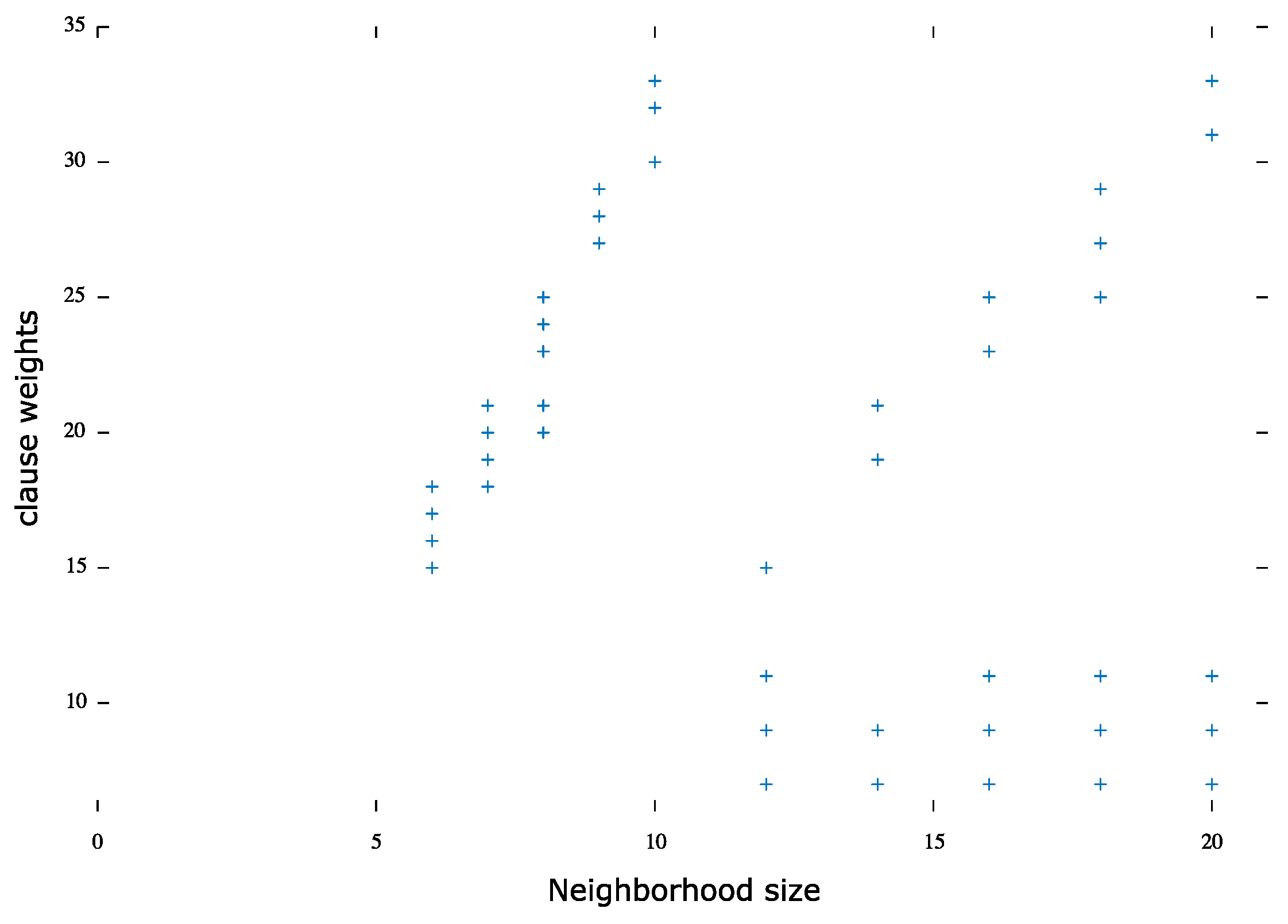
pigeon hole problem set:Figure 1 illustrates the clauses’ weight distribution compared to their neighborhood size for all six instances of the pigeon hole problem. It was indicated that most weighted clauses had a small neighborhood size. Moreover, the statistics showed that 91% of the clauses had less than the average weight where the rest of the clauses, 9%, were weighted the most.

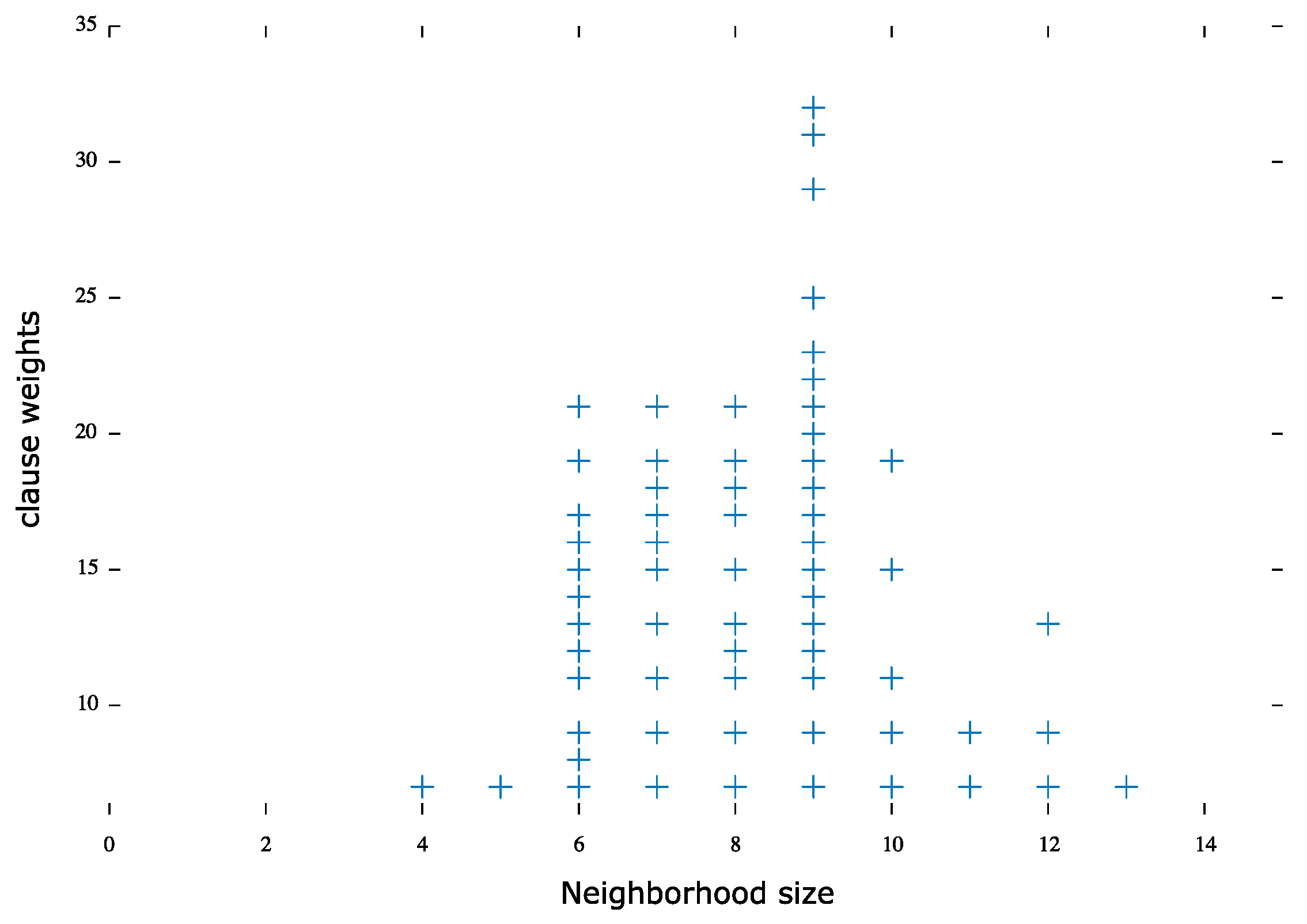
AIM problem set: Similar to the pigeon hole problems, the most weighted clauses were in small neighborhoods. Eighty-six percent of the least weighted clauses had a neighborhood size greater than the average, where 14% had a smaller than average neighborhood size, as illustrated in Figure 2.

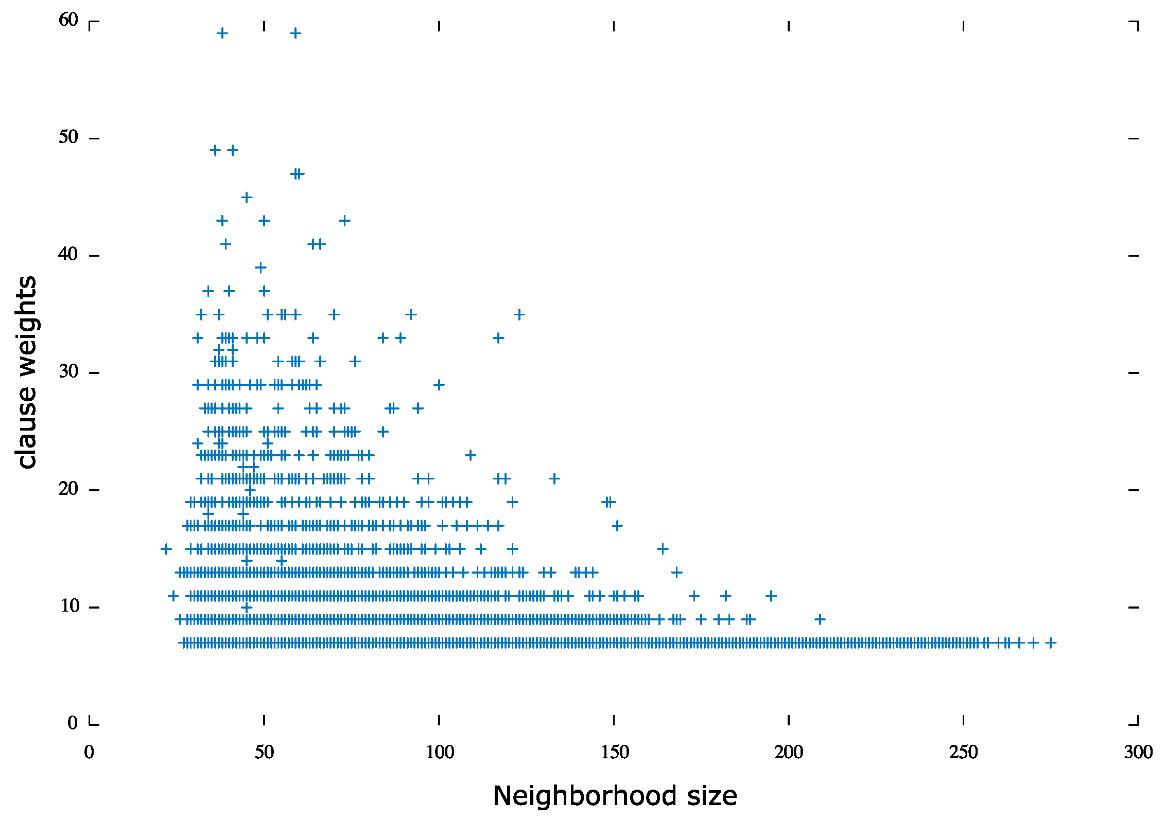
jnh problem set: jnh was of particular interest as the correlation between the clause weights and their corresponding neighborhood sizes was very explicit. Figure 3 illustrates the correlation, as most weighted clauses, specifically 21% of the clauses, had a small neighborhood size 79% of the clauses were the least weighted clauses with a large neighborhood size.

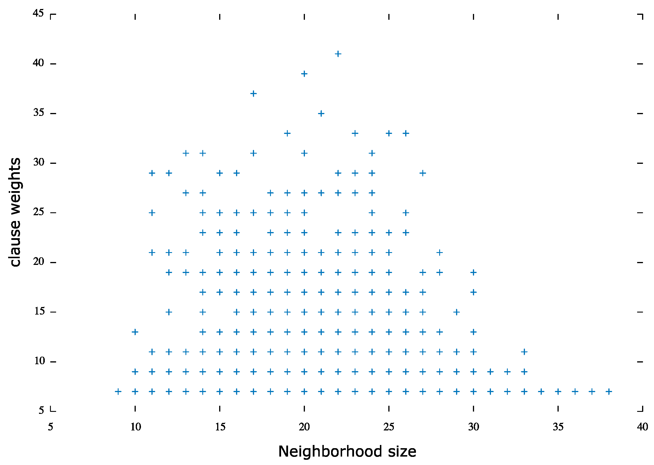
uuf problem set:Figure 4 illustrates an overview of the uniform unsatisfiable problem set weight distribution where 83% of the clauses were least weighted with the large neighborhood and 17% of the clauses were most weighted and had a small neighborhood size.

4.3. Results and Analysis

Our initial expectation before starting our research was that dynamically allocating initial weights could have an impact on the performance level of algorithms that use weights when applied to handling MaxSAT. Moreover, our expectations became more logical due to the statistics extracted from the second step and linking them with the first step mentioned above. Therefore, we experimented with the dynamic weight distribution mechanism on the problems mentioned in Section 4.1. The experiment included recording the results of all the selected algorithms that proved their outstanding efficiency in addressing and solving SAT problems, DDFW, YalSAT, ProbSAT, and Sparrow. In more detail, we modified DDFW+InitWeight, such that instead of stopping upon reaching a solution in which the number of unsatisfied clauses was zero, DDFW+InitMaxSAT stopped if a certain cut-off number of flips was reached or timed out. Moreover, all algorithms were also modified to record the best solution reached (the maximum number of satisfied clauses or the minimum number of unsatisfied clauses) and the time taken to reach that solution. The experiments were performed on an iMac I5 with a 2.5 GHz CPU and 16 GB of RAM. To decide the cut-off, we allowed DDFW+InitMaxSAT a single trial on all the problems with a 20,000,000 flip cut-off. The best cost (maximum number of satisfied clauses) was recorded then it was used for the full experiments. All the solvers were then allowed 1000 runs on each instance. The termination of each run was performed by either reaching the flip cut-off or after 10 s.

Table 2. Average results of the problem set on 1000 run for each solver; the CPU time recorded for each solver when reaching the optimum solution (maximum number of satisfied clauses).

Problems	DDFW	DDFW+InitMaxSAT	YalSAT	ProbSAT	Sparrow
pigeon	0.65	0.04	0.21	0.22	0.45
aim	1.03	0.54	0.97	0.67	0.77
jnh	1.01	0.04	0.62	0.78	0.05
uuf	2.23	0.98	1.76	1.31	1.84

shows the algorithms’ CPU run time when they were applied to MaxSAT problems. We decided to choose DDFW and its variant, DDFW+InitMaxSAT, in our experiment. Furthermore, the study included the experimental results of three other algorithms, YalSAT, Sparrow, and ProbSAT. Firstly, as mentioned above, our choice of DDFW to implement the InitWeight mechanism was that it did not need parameter tuning. The reason for choosing the other three algorithms was that they were the most closely related algorithms to our algorithm, in their method of using weights and solving steps. The ProbSAT algorithm depends on a simplified method, mostly depending on the number of clauses that may become unsatisfied, in deciding to change one of the variables’ value. ProbSAT uses a set of parameters in which an automated mechanism is used to reach their ideal values. We relied in this research on the default values of the parameters published in [26]. As for the YaleSatalgorithm, the experiment indicated that it was more sensitive to the parameter settings when the search process had to be restarted and whether the restart had to start over by assigning random values to the variables or using the clause sizes to determine the value of the weight that should be assigned. Like our approach, YalSAT considers the size of clauses and their neighborhood size to decide on the amount of weight to be allocated to the clauses during the search process. Here, we would like to point out that this difference is fundamentally from the mechanism we presented in this research, as our mechanism allocated the initial weights dynamically before starting the search process instead of through the search process. As for the Sparrow algorithm, weights were used in selecting the variables that appeared promising and that, by changing their value, could lead to reaching partial solutions that were better than the current solution. Sparrow is distinguished because it relies on two properties to determine the probability of choosing one of the weighted variables to change its value (see [27]). We want to emphasize that parameter tuning for this study’s algorithms was not allowed to ensure fairness.

In general, the problem sets were chosen randomly to show the impact of the InitWeight mechanism on the performance of DDFW when applied to handling MaxSAT problems and how it compared to YalSAT, ProbSAT, and Sparrow. Overall, DDFW+InitMaxSAT had the best average performance on all problem sets. In more detail, DDFW+InitMaxSAT had a better average CPU time in comparison to DDFW. Furthermore, DDFW+InitMaxSAT performed better in all problem sets inclusively, as shown below.

pigeon hole problem results: DDFW+InitMaxSAT performed ≈5 times better than YalSAT, ≈2.5 times better than ProbSAT, and ≈2.4 times better than Sparrow.

AIM problem results: For the aim problems, DDFW+InitMaxSAT’s performance was better than YalSAT, ProbSAT, and Sparrow by ≈1.5 times.

jnh problem results: For the jnh problem results, the performance gains by employing the InitWeight mechanism were more significant due to the ratio of variables to clauses where the number of clauses was between 800 and 900 and the number of variables was 100. DDFW+InitMaxSAT was ≈15 times better than YalSAT, ≈20 times better than ProbSAT, and ≈two times better than Sparrow.

uuf problem results: The uuf problem set results were similar to the results of the aim problem sets where DDFW+InitMaxSAT performed better than the other algorithms by ≈1.5 times.

5. Conclusions

An investigational study to examine and verify the performance efficiency of adopting the dynamic initial weight assignment in solving MaxSAT problems was proposed and discussed in this paper. The experimental findings showed that the initial weights’ dynamical assignment positively impacted the DDFW algorithm’s performance. The positive impact was observed and validated through the application of the proposed mechanism to solve MaxSAT problems mentioned in this study, as well as through the comparison with the state-of-the-art algorithms, which proved its effectiveness in addressing similar problems. More specifically, the results in Table 2 showed that DDFW+InitMaxSAT gained 33% over DDFW and performed twice as well as YalSAT and 53% better than ProbSAT, while being 51% better than Sparrow. It should be noted that the results of this study were related only to the problems addressed in the study. Therefore, in our future work, we will aim to extend this research to cover a broader range of problem sets from the Weighted Partial MaxSAT (WPMS) and the Partial MaxSAT (WPS) sets.