Improved Hydraulic Simulation of Valve Layout Effects on Post-Earthquake Restoration of a Water Distribution Network

Abstract

To restore water pipes damaged by earthquakes, it is common to block the water flow by closing the associated shut-off valves. In this process, water supply suspension in the area connected to the isolated pipes is inevitable, which decreases the serviceability of the water distribution network (WDN). In this study, we identified the impact of valve layout (i.e., number and location) on system serviceability during a seismic damage restoration process. By conducting a pressure-driven-analysis (PDA) using EPANET 3.0, a more realistic hydraulic analysis could be carried out under the seismically damaged condition. Furthermore, by considering the valve-controlled segment in the hydraulic simulation, a more realistic water suspension area was determined, and efficient seismic damage restoration strategies were identified. The developed model was implemented on a WDN to demonstrate the effect of valve layout on the post-earthquake restoration process. Finally, effective restoration strategies were suggested for the application network.

1. Introduction

Earthquakes cause massive damage to lifeline systems, such as water distribution networks (WDNs), sewer systems, power lines, gas lines, and roads/bridges. In particular, a WDN is vulnerable to earthquakes and difficult to recover as the majority of its facilities are underground.

Generally, there are two approaches to reduce the seismic damage to WDNs. The first is to enhance system durability to minimize the immediate degradation of the system’s performance from the event. The development of seismic-proof design via advanced reinforcement is advantageous because of the unpredictability of earthquake occurrences [1,2]. The second is to increase the resilience of the system through post-earthquake recovery. Since natural disasters are not entirely preventable, it is essential to improve system resilience in terms of post-recovery to avoid long-term losses. As it is not possible to fully prepare for earthquakes, it is important to establish post-earthquake restoration plans to promptly recover from seismic damage. To replace broken pipes, flow through the damaged pipes is blocked by closing the relevant shutoff valves before restoration work. However, as the number of valves is limited in the actual network, water suspension is inevitable when recovering the system, which leads to a reduction in the water serviceability of the system. Therefore, it is necessary to consider the service suspension area when establishing a recovery strategy for the damaged network.

Several representative studies for the analysis and management of water networks under seismic disasters are summarized as follows. Tabucchi et al. [3] simulated the 1994 Northridge earthquake that occurred in Los Angeles, California using a seismic damage simulation model. The study demonstrated that the sequence and phases of a restoration process can be estimated accurately through modeling but did not attempt to propose or evaluate diverse recovery measures. Bristow and Brumbelow [4] developed a methodology for the vulnerability analysis of water distribution systems under various complex-disaster scenarios. The developed methodology was used to design mitigation measures reducing the consequences of complex disasters. Bałut et al. [5] developed a framework to schedule repairs in water pipe networks for post-disaster responses and restoration services. The developed framework ranks the damaged pipe repair order using a multicriteria decision method. Zhang et al. [6] proposed a dynamic optimization framework using the genetic algorithm to determine the near-optimal sequence of recovery actions for a post-disaster water network and evaluated the resilience using six different metrics. Using a real-world water network with 6064 pipes, they demonstrated the utility of the proposed optimization framework in handling the complex optimization problem.

There are several typical seismic damage quantification models for WDNs. HAZUS [7], developed by the Federal Emergency Management Agency, and MAEviz [8], developed by the Mid-America Earthquake Center, are computer models that quantify the damage to social infrastructures with social and economic values. However, these models do not include restoration measures or system performance simulation. Other examples include GIRAFFE (Graphical Iterative Response Analysis of Flow Following Earthquakes), developed by Shi et al. [9], and REVAS.NET (Reliability EVAluation model for Seismic hazard for water supply NETwork), created by Yoo [10]. In the case of GIRAFFE and REVAS.NET, the damage to a WDN caused by the earthquake is quantified by an indicator of available demand or serviceability through hydraulic analysis. However, GIRAFFE lacks hydraulic modules that describe the detailed hydraulic behavior of damaged WDNs. REVAS.NET focuses on estimating the system reliability for seismic damage. Both models are not equipped to simulate a detailed post-earthquake recovery process.

Later, Klise et al. [11,12] introduced the Water Network Tool for Resilience (WNTR), a new open source Python package designed to help water utilities investigate water service availability (WSA) and recovery time based on earthquake magnitude, location, and repair strategy. The study mainly focused on developing a new model, and simulations to compare and analyze diverse restoration strategies suitable for a damaged network were not conducted.

Recently, Choi et al. [13] developed a post-earthquake simulation model to investigate various recovery strategies. However, the model has two shortcomings; it does not consider the valve layout and relies on a quasi-pressure-driven-analysis (quasi-PDA) for the hydraulic simulation of abnormal network conditions.

Hydraulic analysis approaches are divided into demand-driven-analysis (DDA) and pressure-driven-analysis (PDA) approaches. The DDA assumes that all nodal demands are satisfied regardless of nodal pressure, thereby leading to unrealistic results, such as negative pressure. Meanwhile, the PDA yields more realistic results in an abnormal condition analysis by simultaneously calculating the nodal pressure and available demand. Bhave [14] first proposed the concept of PDA by creating a virtual reservoir at a node of insufficient water pressure. PDA has been actively studied by many researchers recently. Giustolisi et al. [15,16], Wu et al. [17], Baek et al. [18], Tanyimboh and Templeman [19], Giustolisi and Walski [20], and Liserra et al. [21] suggested PDA models with head–outflow relations (HOR) and applied the models to the analysis of real WDNs. Lee [22] proposed an advanced PDA model with the global gradient algorithm (GGA). These PDA models show more realistic results under abnormal operation conditions compared to the DDA.

Regarding the segment analysis of WDNs, Jun and Loganathan [23] proposed a segment search algorithm in WDNs. In their study, the isolated segment was divided into intended isolation and unintended isolation. The intended isolation area (IIA) is defined as the segment where the water supply is cut off along the broken pipe due to the valve shut-off. In contrast, the unintended isolation area (UIA) is defined as the segment where water supply is unintentionally blocked from water sources due to the IIA. The segment search algorithm has been applied in many studies, such as those by Li and Kao [24], Giustolisi and Savic [25], Creaco et al. [26], Alvisi and Franchini [27], Mahmoud et al. [28], and Hernandez and Ormsbee [29]. Recently, Lim and Kang [30] improved the algorithm to search for the UIA and proposed an optimal valve layout that minimizes water suspension.

This study aims to improve the previously developed post-earthquake recovery simulation model by Choi et al. [13]. The improved model is equipped with the full-PDA and valve-controlled segment analysis schemes. The improved model can accurately simulate the pressure-deficient hydraulic conditions and depict water supply interruption by valve isolation during the seismic-damage repair work. The model is then applied to a real WDN to evaluate various scenarios (valve installation cases and recovery strategies) and propose the most efficient restoration strategy for the application network. The methodologies, including the model overview and the improved features in the current study, are discussed in Section 2. The application of the proposed model is provided in Section 3, along with the simulation results. Conclusions and future research directions are discussed in the final section.

2. Methodology

2.1. Model Overview

In this study, we improved the previously developed seismic damage restoration simulation model [13] to analyze the WDN seismic damage restoration pattern according to the valve distribution (number and location). The developed model performs a virtual simulation of the seismic damage and restoration process in a WDN using a full-PDA featured in EPANET 3.0 [31], which is an open-source piece of hydraulic software available online. The model works in conjunction with MATLAB [32] to simulate earthquake occurrence, damage, and the restoration of the WDN. 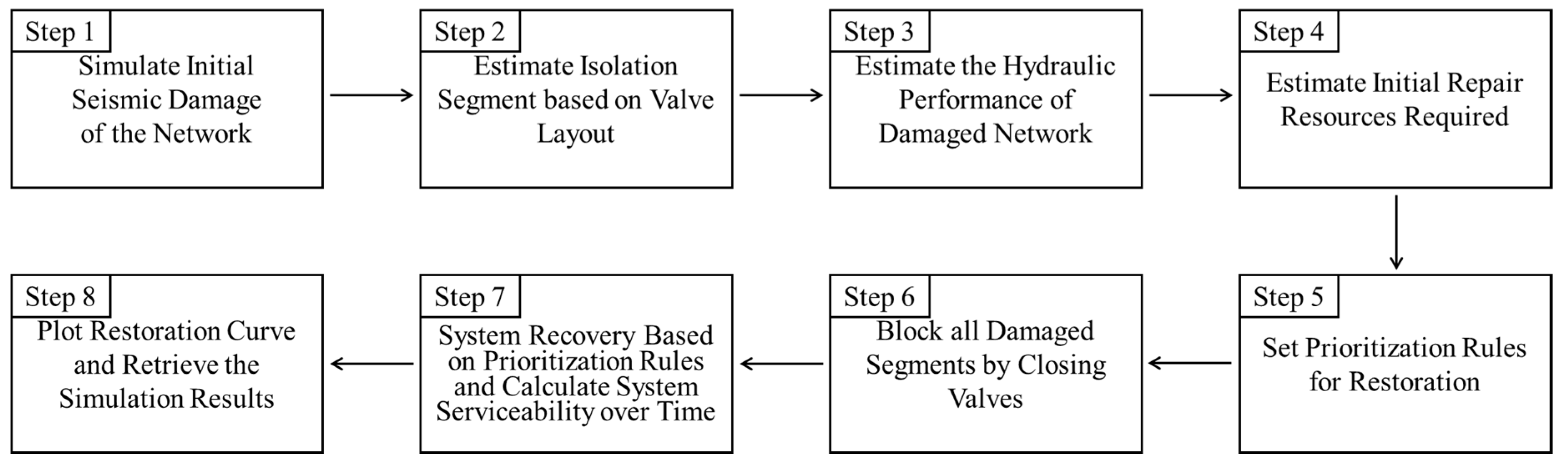As shown in Figure 1, the restoration simulation process of the model consists of eight steps, as described below. More details about the model can be found in our previous work [13].

Step (1): Simulate the initial seismic damage of the network for a given earthquake magnitude and location. The damage states of the components of the system (pipe, pump, reservoir, and tank) are determined based on the seismic location, magnitude, attenuation of seismic waves, and fragility curve.

Step (2): After identifying the valve locations in the damaged network, estimate the isolated segment (water suspension area) based on the location of the damaged pipes and shut-off valves.

Step (3): The damage states of the components (Step 1) and segment data (Step 2) are input to the hydraulic solver (EPANET 3.0), and the hydraulic performance of the damaged network is estimated, which is the initial state of the network immediately after an earthquake.

Step (4): Once the damage state of the system is estimated, calculate and input the necessary restoration resources including repair crews, equipment, and recovery materials. The repair time for the damaged component is also provided. In this study, only recovery personnel were simulated (for primary emergency recovery).

Step (5): After inserting the available recovery resources, set up recovery priority rules such as the prioritization of the recovery and transfer methods of recovery personnel.

Step (6): Before proceeding with the system recovery, shut off the water flow through the damaged pipeline by blocking the segment as per the valve layout (Step 2).

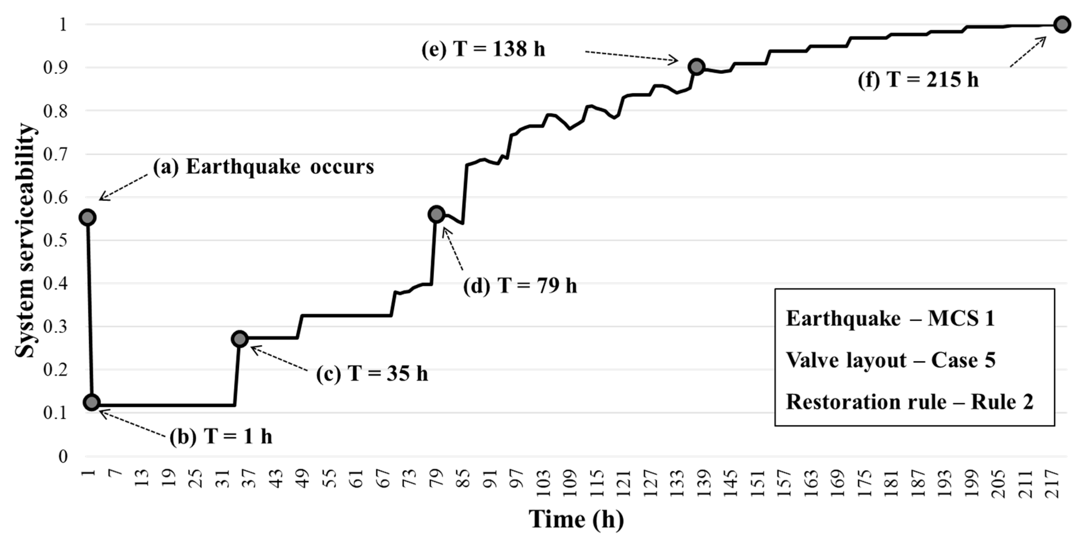
Step (7): Begin system recovery according to the pre-determined recovery rule (Step 5). The damaged pipes are replaced according to the recovery rule set in Step 5, and when all damaged pipes in the segment are replaced, the blockage of that area is dismantled. In this manner, consider that the variation in the water suspension area due to the restoration process goes on, and calculate the system serviceability over time and quantify the restoration degree. The travel time of the repair crews is estimated based on the recovery order and travel route. The recovery continues until the primary emergency recovery (the replacement of the broken pipes) is completed.

Step (8): Once the emergency recovery is completed, simulation results such as system serviceability over time, recovery crew activity statistics, and a spatio-temporal map of recovery progress are presented, and the model simulation is completed.

2.2. Seismic Damage Simulation

2.2.1. Tank and Pump

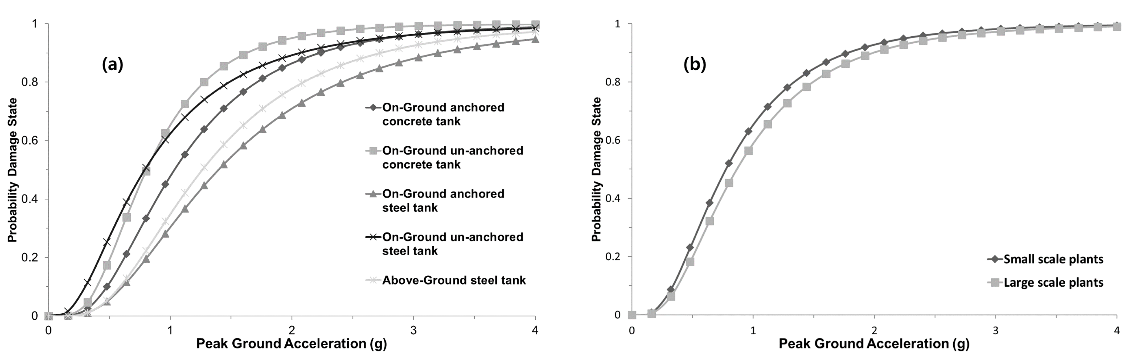
The facility (tank and pump) damage caused by an earthquake can be determined using the peak ground acceleration (PGA) and the fragility curve. The PGA indicates how strongly the ground shakes and is affected by the seismic waves reaching the facility. The fragility curve shows the probability that the extent of a facility’s damage is beyond a certain level as a function of the PGA. Figure 2 shows the fragility curves applied to determine the damage status of tanks and pumps, which were presented in the Seismic Fragility Formulations for Water Systems Part 1 Guidelines [33]. The y-axis indicates the probability that the facility incurs damage when the PGA value of the seismic wave corresponds to the x-axis. The “on-ground anchored concrete tank” and a “small-scale plant” were assumed for the tank and pump types in our model, respectively. Note that different fragility curves should be applied depending on the facility types and sizes.

The model classifies the damage of the facility (tank and pump) into two types, damaged (function stopped) or normal. The facility damage determination steps are as follows.

Step (1): Calculate the PGA at each facility using the seismic wave attenuation equation (see Choi et al. [13] for details of the formula). The PGA is determined based on the magnitude of the earthquake and distance from the epicenter.

Step (2): Calculate the probability of damage of each facility using the estimated PGA value and the fragility curves (Figure 2).

Step (3): Generate a random number between 0 and 1 for each facility. If the random number is smaller than the damage probability estimated in Step 2, the facility is identified as “damaged”, otherwise, “normal”.

The repair time of a tank ranges from 24 to 36 h, and that of a pump, 8 to 12 h. For the hydraulic simulation of damaged tanks and pumps, the model controls the front and rear pipelines directly connected to the damaged facilities to deactivate the water flows. If a tank is damaged, the model closes the discharge pipe; thus, no water can be supplied from the tank. If a pump fails, the pump status is set to “closed”, and the front and rear pipelines of the pump are closed in the model. Once the repair is completed, the closed pipelines and pumps would be set to “open” to simulate the recovery of the facilities.

2.2.2. Pipe

The pipeline damage was determined based on the concept of the repair rate (RR). The repair rate is the number of repairs per unit length of the pipeline and is calculated by peak ground velocity (PGV) and multiple correction factors (C values), as expressed in Equation (1). Note the equation was adopted from ALA [33] and Isoyama et al. [34].

$$\mathrm{RR}=C_1\times C_2\times C_3\times C_4\times 0.00187\times PGV$$

(1)

Here, RR = repair rate (no. of repairs/1000 ft) (1 ft = 0.3048 m) and $C_1$, $C_2$, $C_3$, and $C_4$ represent the correction factors for the pipe diameter, pipe material, topography, and liquefaction, respectively.

The seismic damage to pipelines is divided into breakage and leakage. The breakage indicates that the water flow through the pipe is completely suspended, while the leaking pipe still conveys water with a potential loss of flow and pressure. Here, the pipe damage condition was simulated through the following procedure:

Step (1): Calculate the PGV value at each pipe.

Step (2): Calculate the repair rate (RR) of the pipes using Equation (1).

Step (3): Calculate the interval between repair points (L1 = 1/RR) of each pipe and compare it with the actual pipe length (L2). If L1 is smaller than L2, seismic damage occurs in the pipe; otherwise, no damage is assumed.

Step (4): For the damaged pipe (L1 < L2), a random number between 0 and 1 is generated and compared with the pipe breakage probability computed by Equation (2), which is suggested by ALA [33]. If the random number of the pipe is smaller than the breakage probability, the pipe is tagged with “breakage”, otherwise, “leakage”.

Step (5): Following this procedure, all the pipes in the network are classified into either “no damage”, “leakage”, or “breakage”.

$$P_b=1-e^{-RR\times L}$$

(2)

Here, $P_b$ = the probability of pipe breakage and $L$ = the pipe length (ft).

The replacement time of a broken pipe was estimated using the empirical formula suggested by Chang et al. [35], as expressed in Equation (3). As shown in the equation, the replacement time is generally proportional to the pipe diameter, with a preparation time of 2 h.

$$t_b=\frac{D}{100}+2$$

(3)

Here, $t_b$ = replacement time for a broken pipe (h) and D = pipe diameter (mm).

Water loss by leakage and breakage is a pressure-dependent flow and is expressed by Equation (4), which was proposed by Puchovski [36]. In the model, the EPANET emitter option at a node was used to simulate the water loss from the damaged pipes.

$$\mathrm{Q}=C_d{P}^{0.5}$$

(4)

Here, Q = the water loss through leaks/breaks; $C_d$ = the discharge or emitter coefficient in EPANET and is given by ${\left(\frac{2g}{{\gamma }_w}\right)}^{0.5}A$, in which $g$ = gravitational acceleration, ${\gamma }_w$ = the specific weight of water, and $A$ = the opening area of the damaged pipe; and $P$ = the nodal pressure. The total opening area ($A$) of the leaks is assumed to be 10% of the cross-sectional pipe area.

For the hydraulic simulation of the damaged pipes, the discharge coefficient ($C_d$) is calculated first. For a broken pipe, $C_d$ is assigned to the upper node of the pipe in the flow direction, and the pipe status is set to “closed”. Meanwhile, a pipe with leaks may partially lose its function but still conveys water, $C_d$ is assigned to the downstream node of the flow direction, and the pipe status is still “open”. Once the replacement of the damaged pipes is completed, the closed pipelines would be set to “open”, and the assigned emitter option is removed.

The above-mentioned damage conditions of the WDN components are determined, and EPANET hydraulic analyses are conducted to quantify the water supply capacity of the network. Here, the water supply capacity is estimated as the amount of water that is actually supplied to end users under the seismic damage condition. Note that more details about the hydraulic modeling process can be found in our previous study [13].

2.3. Model Improvements

2.3.1. Hydraulic Simulation Using PDA

In our previous model [13], quasi-PDA simulation was performed using EPANET 2.0 [37] as a hydraulic solver. The quasi-PDA artificially removes negative pressure by repeatedly performing DDA analysis. That is, if negative pressures occur in the network when performing DDA, the base demand of the relevant nodes is set to zero (which means that no water can be supplied to the nodes); then, the DDA hydraulic simulation is performed again. The above steps are repeated until the negative pressure no longer occurs in the network. The quasi-PDA simulates an abnormal situation by DDA-based hydraulic simulation; however, the system serviceability is moderately underestimated by suppressing the negative pressure nodes. To address the limitations of quasi-PDA and to accurately simulate the hydraulic conditions of abnormal situations, this study performed full-PDA by linking the model with the EPANET 3.0 solver [31]. By improving the quasi-PDA option of the previous model to the full-PDA option, the drops in water pressure due to seismic damage and the actual available water supply can be estimated more accurately. Thus, a more realistic and accurate hydraulic simulation was achieved in abnormal seismic damage situations. The actual available water supply ($Q_{avl}$) calculated using the PDA of EPANET 3.0 is utilized in Equation (5), which is an estimation of the system serviceability index presented by Shi [38] and Wang [39].

$$S_s=\frac{{{\displaystyle \sum }}_{i=1}^N{Q}_{avl,i}}{{{\displaystyle \sum }}_{i=1}^N{Q}_{req,i}}$$

(5)

Here, $S_s$ is the system serviceability index, $Q_{avl,i}$ and $Q_{req,i}$ are the available (or serviceable) and required demand at node i, respectively, and $N$ is the total number of nodes.

2.3.2. Segment-Based Isolation Simulation

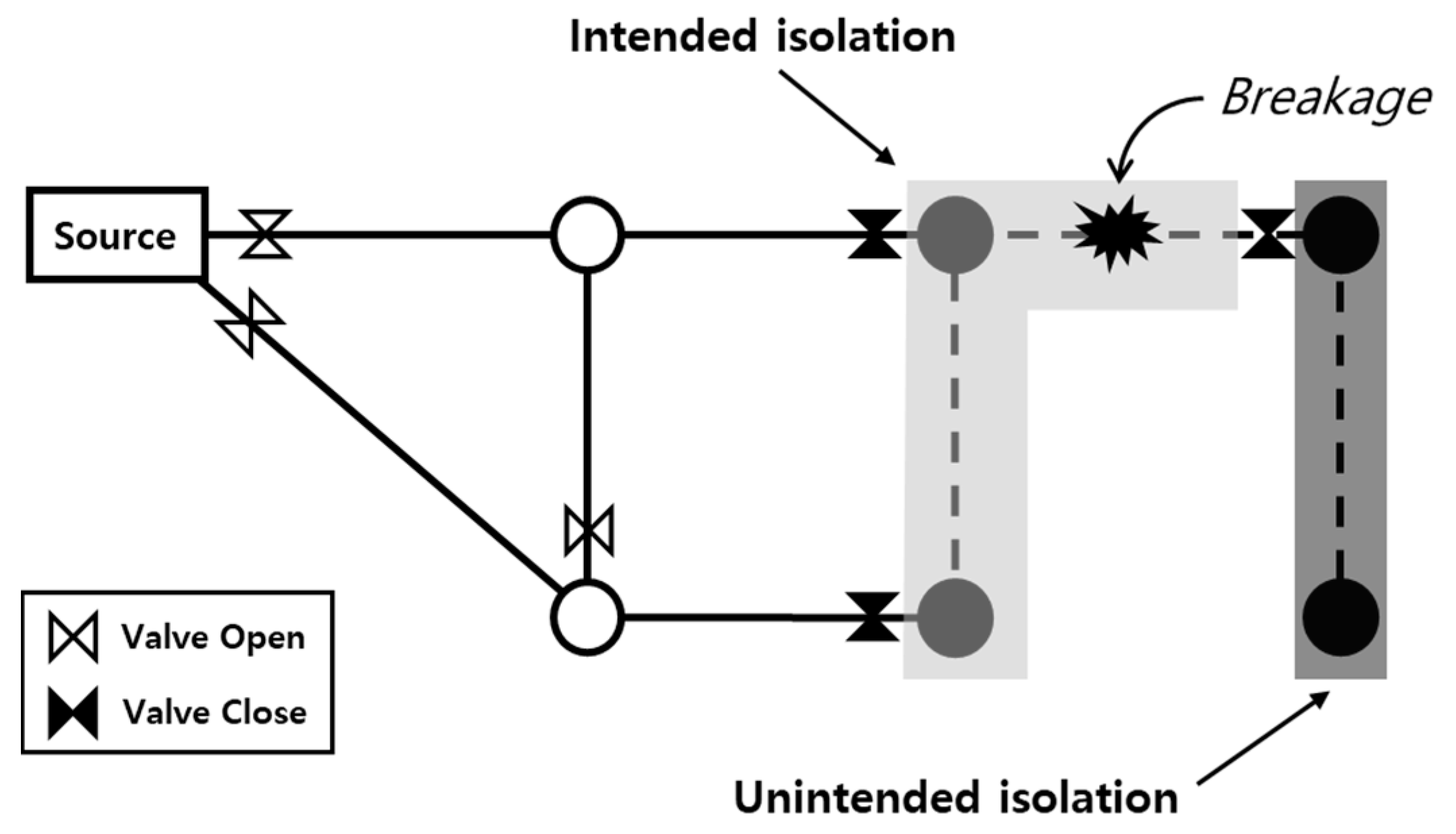
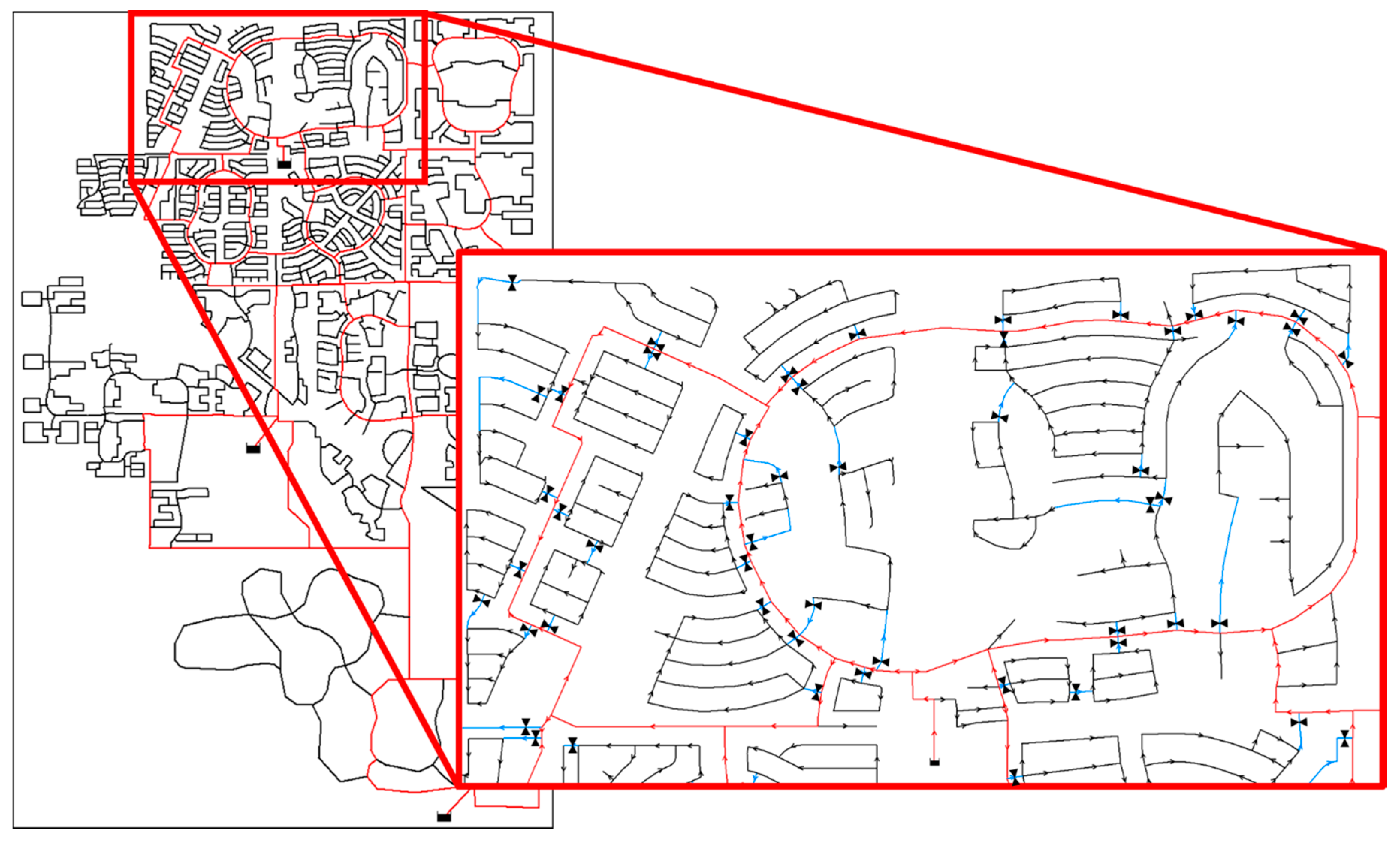
The restoration and replacement of pipes damaged by an earthquake usually proceed after the area is isolated from the system by shutting off the valves adjacent to the damaged pipe. In this case, as shown in Figure 3, the service suspension area—in which the water supply, along with the broken pipe, is cut off—is defined as an IIA, and the area where water supply is unintendedly cut off from the water source because of isolating the IIA is defined as the UIA [23]. That is, when the water supply zone is blocked by shutting off the valve for the restoration of the damaged pipe, not only the corresponding area but also the area located downstream of the water flow may be blocked. The range of this service suspension area varies based on the number and location of valves installed in the network, which greatly affects the water supply capacity during seismic damage restoration. In the previous model [13], since it is assumed that valves are installed at both ends of all pipes, which is unlikely in a real system, the system serviceability is overestimated because the service suspension area and the water suspension capacity are not reflected during the damage restoration. This study reflects the valve position installed in the network to simulate the water suspension situation arising from seismic damage more realistically. This enabled the estimation of the direct and indirect service suspension area according to the locations of the damaged pipes and valves and the accurate calculation of system serviceability. In this study, the method presented by Lim and Kang [30] was applied as the IIA and UIA search algorithm.

2.4. Summary of Assumptions and Limitations

The assumptions used and limitations contained in the development and application of the model are summarized as follows. (1) The application of the model is limited to the water pipe network only; thus, interconnections with other lifeline networks (electric power, transportation, telecommunication, etc.) were not considered. (2) The recovery equipment (crane, excavator, truck, etc.) and material usage (mechanical couplings, pipe sections, repair champs, etc.) were not considered in the simulation. Only the recovery personnel activity was simulated. (3) The transportation speed limit of the recovery personnel was set to 10 km/h by assuming that road conditions are abnormal due to seismic damage. (4) The recovery simulation only considered the replacement of broken pipes. In general, locating and repairing the leaks is more challenging and time-consuming compared to that of the breaks and was excluded from the simulation. (5) The water quality deterioration in the network was not considered. (6) Valve failure due to seismic damage was not considered. (7) The restoration starts only after the segments are blocked by valve closure, and the time required for valve closure was not considered. (8) All the pipes were considered to be accessible for valve installation, which may not be true in real cases.

3. Applications and Results

3.1. Application Network

For demonstration purposes, the developed model was applied to a mid-size WDN, shown in Figure 4. The application network consists of three reservoirs, 1112 nodes, and 1459 pipes, and the total base demand of the system is about 50,370 m³/day. Note that there is no tank and pump installed in the application network. The size of the pipe ranges between 150 and 400 mm. The number of 150 mm pipes was 542, which is approximately 37% of the total number of pipes. The total number and length of pipes per diameter are summarized in

Table 1. Pipe size distribution of the application network.

Diameter (mm)	150	200	250	300	400	Total
Count	542	401	253	260	3	1459
Length (m)	115,910	70,714	48,854	63,903	352	299,733

.

3.2. Model Applications

We simulated a virtual earthquake occurrence in the central area of the application network. The seismic intensity is assumed to be of 7.0 magnitude on the Richter scale, and the depth of the epicenter is assumed to be 10 km. A sensitivity analysis was performed by configuring the valve distribution in various cases to compare and analyze changes in seismic damage restoration patterns according to the valve layouts. In general, valves are installed at the front and rear of operational facilities (e.g., reservoirs, tanks, and pumps) or on boundary pipes to distinguish the district metered area (DMA). The main purpose of the DMA is the early detection and management of leakage to reduce nonrevenue water in the network. The district isolation can also ease pressure management and protect the network from accident or contamination events. Recently, Giudicianni et al. [40] proposed creating dynamic DMAs that allow for the expansion of existing DMAs to improve network resilience by overcoming the failure events. In this study, the valve locations were determined based on the pipe diameter to objectively compare and analyze the effect of valve layouts on seismic restoration. Figure 5 shows the distribution of pipes in the network per size.

In addition, the valves can be installed at both ends of a pipe or only at one end. For both cases, the range of the service suspension area is different, and the number of valves to be installed also differs two-fold. To identify the impact of these differences, we investigated two cases, with “installation at both ends of a pipe” and “installation at the upstream end of a pipe”. Finally, to consider the segmented network, a case was added in which valves were installed on the main transmission pipes and the boundary pipes. As shown in Figure 6, the boundary pipes, where the valves are to be installed, are usually the pipes through which the water flows into a small block, specifying the boundary between the blocks, and branch from the main lines. Nine valve installation cases constructed for sensitivity analysis are summarized in

Table 2. Comparison of valve installation cases.

Case	Description	No. of Applied Pipes	No. of Installed Valves
1	Both ends of pipes with Dia. ≥ 300 mm	263	526
2	Both ends of pipes with Dia. ≥ 250 mm	516	1032
3	Both ends of pipes with Dia. ≥ 200 mm	917	1834
4	Both ends of pipes with Dia. ≥ 150 mm	1459	2918
5	Upstream end of pipes with Dia. ≥ 300 mm	263	263
6	Upstream end of pipes with Dia. ≥ 250 mm	516	516
7	Upstream end of pipes with Dia. ≥ 200 mm	917	917
8	Upstream end of pipes with Dia. ≥ 150 mm	1459	1459
9	Case 5 & upstream end of boundary pipes	521	521

. In Cases 1–4, valves were installed on both ends of a pipe; in Cases 5–8, valves were installed on the upstream end of a pipe; and in Case 9, valves were installed on the boundary pipes adding to Case 5.

In the seismic damage restoration of a WDN, the restoration progress and efficiency of the entire system can vary greatly depending on the pipe restoration priority rules, as well as the valve installation cases. Therefore, in this study, a sensitivity analysis of the network restoration efficiency according to pipe restoration priority rules was performed. As summarized in

Table 3. Applied system restoration rules.

Rule	Description	Note
1	Pipes carrying higher water flow receive higher restoration priority	Pipe-based restoration
2	Segments with higher water suspension volume receive higher restoration priority	Segment-based restoration
3	Segments with shorter repair complete time receive higher restoration priority	Segment-based restoration
4	Segments closer to reservoirs receive higher restoration priority	Segment-based restoration

, four rules were constructed that were divided into “pipe-based restoration rule” and “segment-based restoration rule”. Rule 1 is a pipe-based restoration rule that preferentially repairs the pipes carrying a higher water flow. Rules 2 through 4 are segment-based restoration rules considering the service suspension areas from valve shutoffs. Under these rules (Rules 2 through 4), the restoration is conducted based on a segment; that is, when all damaged pipes belonging to a segment (i.e., suspension area) are completely replaced, the suspension of the segment is released by opening the associated valves. In Rule 2, the service suspension area with the higher water suspension volume gets a higher priority. In Rule 3, the area with a shorter replacement time (total replacement time required to complete restoration of the damaged pipe in the area) receives a higher priority. According to Rule 4, the service suspension area near the reservoir (source), generally belonging to the upstream part of the network, is preferentially restored.

As a Monte Carlo simulation (MCS), 10 different earthquake events were generated to reflect the diversity of seismic damage that can occur in the application network. Then, the system restoration was simulated using the developed model by applying the abovementioned valve layout cases and system restoration rules.

3.3. Simulation Results

3.3.1. Restoration Efficiency According to Valve Layout

In the first analysis, system restoration efficiencies according to the constructed nine valve layouts were compared and analyzed. For this analysis, the restoration rule, Rule 2, was commonly applied to the nine cases. Figure 7 depicts the system restoration curve in which the x-axis shows the time elapsed since the seismic damage and the y-axis indicates the system serviceability index described in Equation (5). The shaded area represents the serviceability range calculated from the 10 MCS results, and the solid black line represents the average serviceability index of the MCS results. Comparing the shaded area, it can be seen that a larger number of valve installations lead to lower system serviceability drops due to seismic damage and a lower serviceability deviation for various earthquake events (represented by MCS shades). This implies that when the number of valve installations becomes large, there is no significant difference in the restoration efficiency for various seismic events (with a similar magnitude) and the system can cope with the damage at a certain level. Installing as many valves as possible on all pipes will minimize the water suspension area and allow more efficient restoration, but there are economic limitations to valve installation.

In analyzing the effects of the number of valve installations, it can be seen that in Cases 1, 5, and 6, where the number of valve installations is relatively small, the variance in serviceability is larger than that in other cases. The difference in restoration efficiency is large for individual seismic events; i.e., water serviceability is not ensured with such a low number of valves installed in the network. In addition, it can be seen that the decrease in system serviceability immediately after an earthquake is considerably large. This signifies that a large service suspension area is generated initially due to the small number of valves installed. By contrast, in Cases 2–4 and 8, the variance in serviceability (over the different earthquake events) decreases, and the system serviceability drop immediately after an earthquake also decreases significantly. This result implies that even in the various earthquake events, the network can cope with a certain restoration efficiency and is more stable in terms of system serviceability. Through these results, it can be confirmed that if a large number of pipes are damaged due to the earthquake, the number of valve installations has a significant impact on the system restoration.

Comparing valve installation at both ends (Cases 1–4) and the upstream end (Cases 5–8), the cases where valves are installed at both ends of a pipe are more favorable for restoring system serviceability. However, considering that the number of valve installations needs to be doubled, the economic feasibility (i.e., restoration efficiency against cost) of these cases must be examined. In Case 9 (Case 5 + Boundary valves at small block entrance), the number of installed valves is relatively small (521 valves), but it has a considerably higher restoration efficiency than that of other cases with similar numbers of valve installations (i.e., Case 1 with 526 valves and Case 6 with 516 valves). By clustering the water network into blocks, the service suspension area is minimized when seismic damage occurs, enabling appropriate responses and restoration work against damage. If we summarize the above results, the number of valve installations and the efficiency of damage restoration are analyzed to be proportional to each other, and one-end valve installation is regarded to be more cost-effective than installation at both ends of a pipe. In practice, it is deduced that installing valves on the boundary pipes would be the most cost-effective option for damage restoration when network blockage is considered.

3.3.2. Restoration Efficiency According to the Restoration Rule

The second analysis compares and analyzes changes in restoration efficiency according to the restoration rules. For this analysis, the valve installation case should be fixed for each simulation. As shown in the previous analysis, there are no significant differences in restoration efficiency against the different instances of seismic damage in the cases with a large number of valves installed. Thus, Case 5, with the smallest number of valve installations, was used to see the differences in restoration efficiency according to the restoration rule.

Figure 8 shows the system restoration curves indicating the average serviceability of 10 MCS results over time for each of the applied restoration rules. The comparison indicates that the restoration strategy of Rule 2 (priority restoration for segments with high water suspension) tends to progress slowly in the early stage of restoration but shows rapid recovery after the mid-stage of restoration, resulting in higher system serviceability overall compared to other rules. In general, a segment with a large amount of water suspension flow is widely spread in space and requires a longer time to complete the restoration. Therefore, Rule 2 is disadvantageous at the initial stage before completing such segments; however, after such areas are repaired, the system serviceability is greatly enhanced, and shows good overall performance. By contrast, Rule 1, which preferentially replaces pipes with high water flow rates without considering the service suspension area (i.e., segment), shows the most inefficient restoration. This is because, in the case of damage restoration of the network, the service suspension area is released only when the repair work of all the damaged pipes is completed in one service suspension area. That is, when there are multiple damaged pipes in one service suspension area, and the restoration team moves to another area without completing the repairs in the first segment, the service suspension area release is delayed, which is disadvantageous in terms of system serviceability restoration. The smaller the area of the restoration curve (upper part) in Figure 8, the more efficient the restoration is. The analysis indicated that the efficiency of the applied restoration rules could be ranked in the following order based on the curve area: Rule 2 > Rule 3 > Rule 4 > Rule 1. Therefore, the segment-based restoration is more effective than the pipe-based restoration, and among the segment-based restorations, it is more efficient to preferentially restore segments with large water suspension flows.

3.3.3. Comprehensive Analysis

Figure 9 displays a heatmap showing the time-average system serviceability for all valve-layout cases, restoration rules, and seismic events (MCS). Note the time-average system serviceability indicates the average system serviceability from immediately after the earthquake occurrence until the restoration completion. The darker the color, the higher the system serviceability (damage restoration efficiency). Using this chart, the system serviceability can be intuitively identified according to the valve layout and restoration strategy. The most noticeable result is the difference by cases, regardless of the seismic events and restoration rules. The cases with more valve installations display darker colors (higher average system serviceability). In Cases 3, 4, 7, and 8, the average serviceability is over 0.9 for all restoration rules, possibly caused by the larger number of valves installed in the network leading to smaller service suspension areas under the seismic damage and a constant restoration efficiency. This high average serviceability implies that the corresponding valve cases can respond more easily to seismic damage with higher resilience. When comparing the average serviceability according to the valve installation positions, Cases 3 and 4, with valves installed at both ends of a pipe, show a slightly higher average serviceability than that of Cases 7 and 8, where valves are installed at the upstream end. However, as the difference between the two types of case is not large, it can be said that the efficiency is lower, considering the valve installation cost. Case 9 is judged to be the most cost-effective for the application network as it shows high efficiency considering the number of valve installations, by limiting the size of the service suspension area to small blocks at the early stages of the damage.

A comparison of the restoration strategies indicates that Rule 2 shows much higher serviceability (average serviceability 0.886) than that of other rules in all valve-layout cases and MCS, and Rule 1 shows the lowest serviceability (average serviceability 0.810). Variation in system serviceability by restoration rule can be seen in the cases where the number of installed valves is small. That is, when the number of valves installed in the network is small, it can be seen that the restoration efficiency is greatly influenced by how the restoration rule is established. Thus, for the network with limited valves installed, care should be taken to choose the appropriate restoration strategy for efficient seismic damage recovery. By contrast, it can be expected that the network with many valves installed may not have high sensitivity due to the restoration strategy applied.

Summarizing the simulation results for different valve layouts and restoration rules for the application network, Case 9 of the valve layout and Rule 2 of the restoration strategy appear to be the most efficient against various earthquake events.

In addition, an economic analysis was conducted to compare the valve installation costs and the restoration performance of the nine valve installation cases. The valve installation cost suggested by Walski [41] was used, as shown in

Table 4. Valve installation cost.

Size (mm)	Cost (USD)
150	600
200	745
250	1035
300	1210

.

Table 5. Summary of valve installation costs and system serviceability of nine valve-layout cases.

Case	Description	No. of Valve Installed					Valve Cost (USD)	Ss
		Total	@ D300	@ D250	@ D200	@ D150
1	Both ends of pipes with Dia. ≥ 300 mm	526	526	0	0	0	636,460	0.66
2	Both ends of pipes with Dia. ≥ 250 mm	1032	526	506	0	0	1,160,170	0.86
3	Both ends of pipes with Dia. ≥ 200 mm	1834	526	506	802	0	1,757,660	0.95
4	Both ends of pipes with Dia. ≥ 150 mm	2918	526	506	802	1084	2,408,060	0.96
5	Upstream end of pipes with Dia. ≥ 300 mm	263	263	0	0	0	318,230	0.65
6	Upstream end of pipes with Dia. ≥ 250 mm	516	263	253	0	0	580,085	0.81
7	Upstream end of pipes with Dia. ≥ 200 mm	917	263	253	401	0	878,830	0.93
8	Upstream end of pipes with Dia. ≥ 150 mm	1459	263	253	401	542	1,204,030	0.96
9	Case 5 & upstream end of boundary pipes	521	263	0	0	258	473,030	0.86

summarizes the valve installation cost and the system serviceability of each case. Note that the system serviceability (Ss) is estimated by averaging the serviceability values of all MCS scenarios and restoration rules of each case. As seen in the table, Case 9 shows relatively high system serviceability with the second lowest investment, indicating the most cost-effective valve layout. It is interesting to observe that Case 2 shows the same system serviceability (Ss = 0.86) as Case 9 but the cost is 2.5 times higher than that of Case 9. Compared with Cases 1 and 6, Case 9 is superior in terms of both of cost and restoration performance.

3.3.4. Visualization of Spatio-Temporal Restoration Progress

The developed model provides a spatio-temporal recovery map that visualizes the restoration progress of a network in time and space. Figure 10 illustrates the results of applying Case 5 for valve layout and Rule 2 for restoration strategy under the seismic event of MCS 1. From the system restoration curve and the spatio-temporal recovery map illustrated in Figure 10, it is easy to understand the overall restoration progress after a damage occurrence. Firstly, it can be seen that system serviceability decreases sharply between points (a) and (b). The time point (a) is immediately after the earthquake, and before the segment is isolated; thus, the water flows out through the damaged pipes, reducing the overall network serviceability. At point (b), all service suspension areas were isolated by shutting off the valves corresponding to the area containing the breakage pipes, resulting in very low water supply (system serviceability (Ss) = 0.118), because most of the network was isolated (except for some areas in the north and south). As the restoration of the damage pipes proceeds, the system serviceability increases from point (c) through (f). The system serviceability curve shows a gradual increase with time; in particular, at time points (c) and (d), which are at the early stages of restoration, the curve shows a rapid increase. These results are evident in the spatio-temporal recovery map. The rapid increase is due to the release of water suspension after the repair of the large service suspension area is completed at that time point. Subsequently, service suspension areas with relatively small sizes were continuously restored, and at about 138 h after the start of the restoration (point (e)), approximately 90% of the water supply was restored. Finally, all restorations were completed by about 215 h after the recovery initiation (point (f)). The spatio-temporal recovery map can assist the system managers in assessing the expected service suspension area, expected restoration completion time, serviceability at individual nodes, and restoration progress of the entire network over time after an earthquake. Using these features, the model can be used as a decision-making tool for various purposes, such as pre-reinforcement planning in areas where high water suspension is anticipated by installing additional valves, and planning to prioritize critical areas (hospitals, government offices, factories, etc.) within the network by a criticality-based network restoration strategy.

4. Conclusions

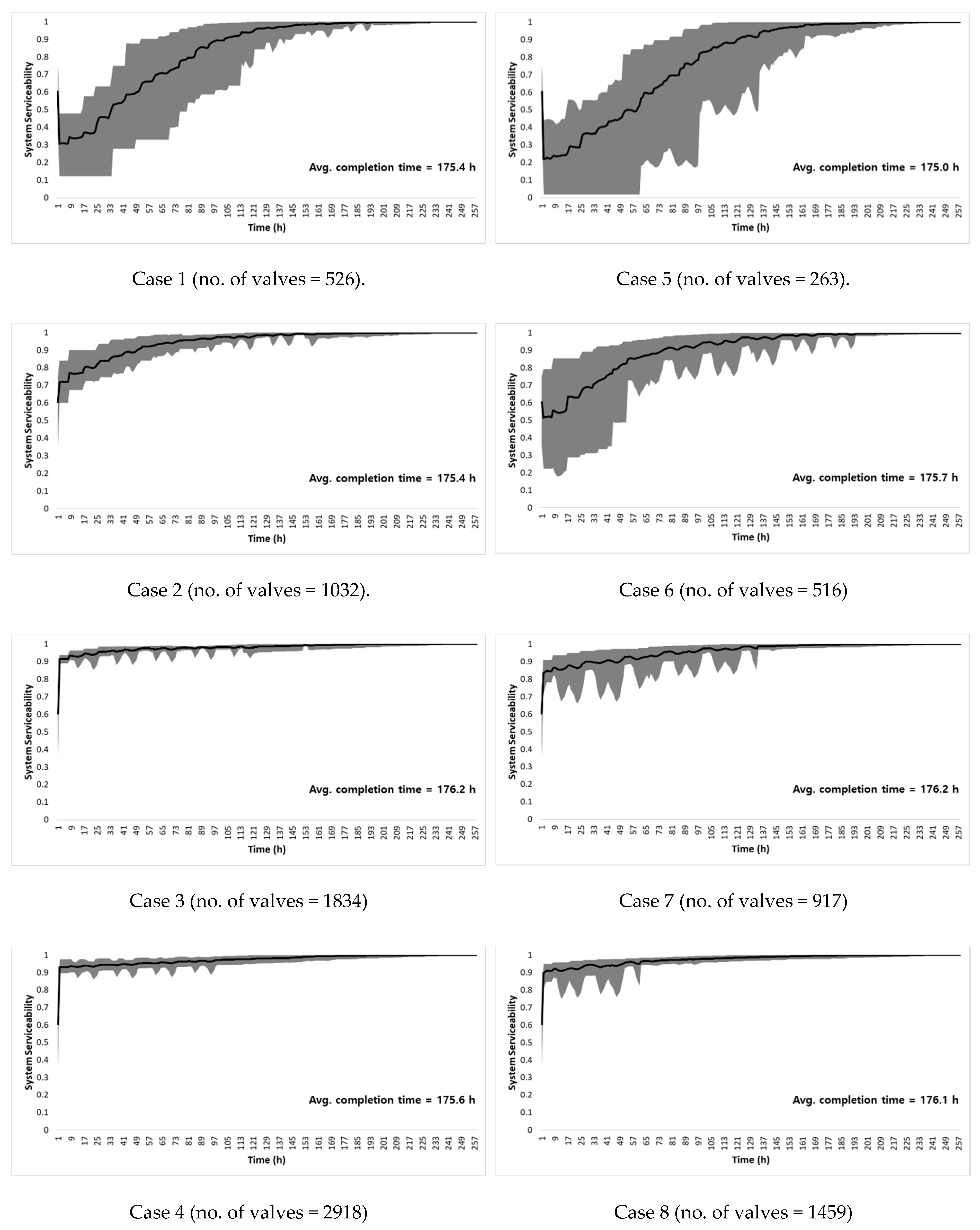
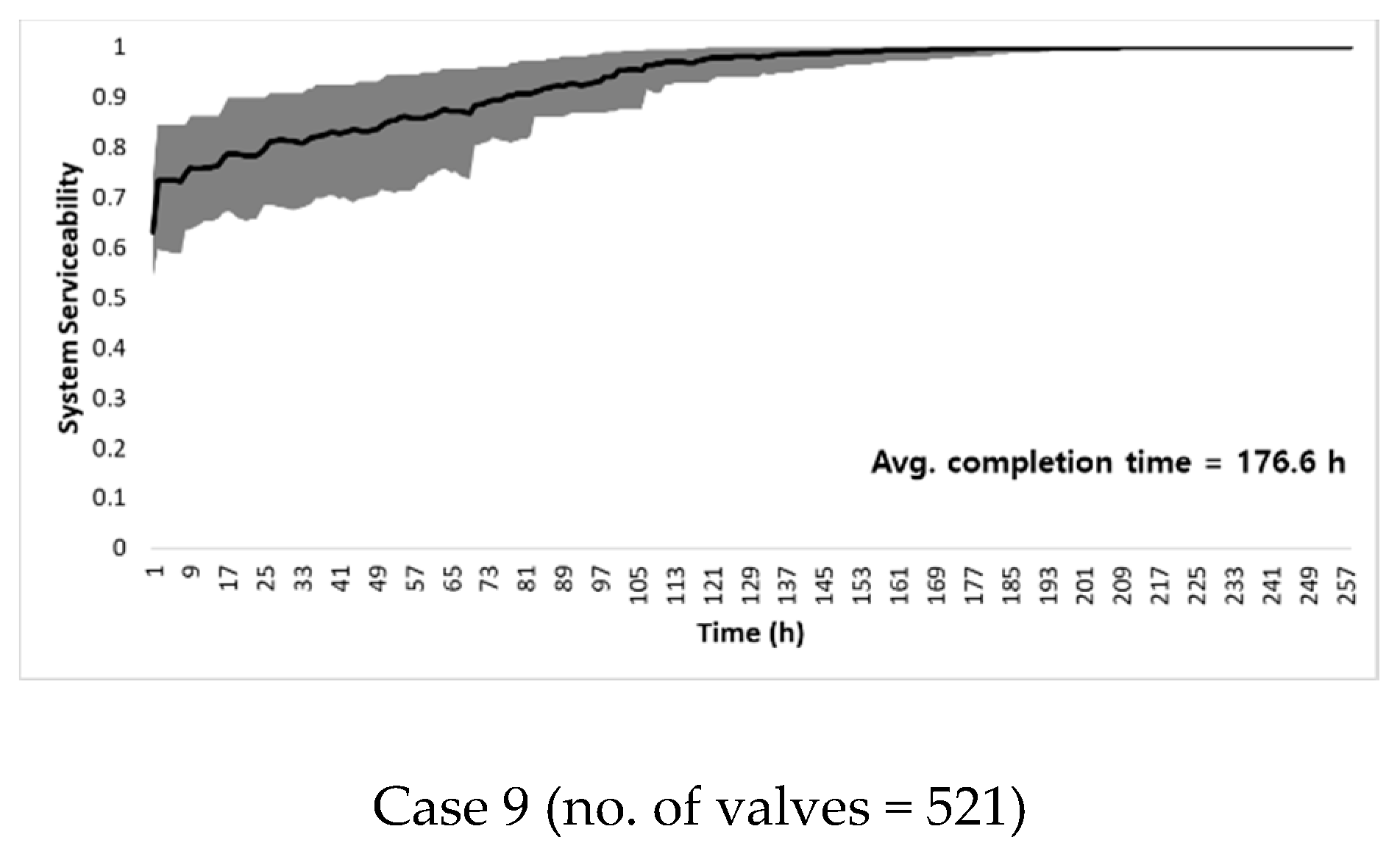
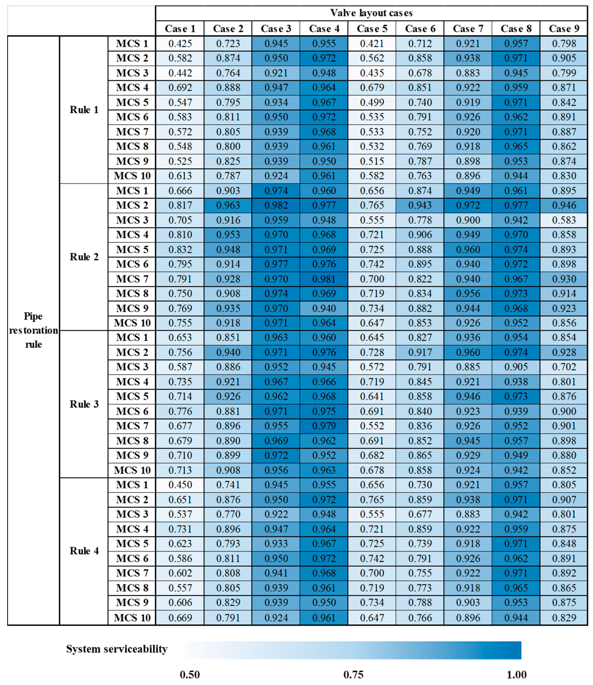
In this study, we aimed to improve our previous model by incorporating the valve-controlled segment algorithm and full-PDA hydraulic solver. The improved model enables accurate hydraulic simulation under seismic damage situations and identifies the service suspension area caused by intentional valve shut-off. The improved model enables a more realistic simulation of seismic damage and restoration processes in a WDN. Here, the improved model was applied to a real WDN, and the effects of the valve installation layout (number and location) and the pipe restoration rules on the seismic restoration efficiency were analyzed. The sensitivity analysis results according to the nine valve-layout cases and four restoration rules, applied for 10 earthquake events of MCS, are as follows.

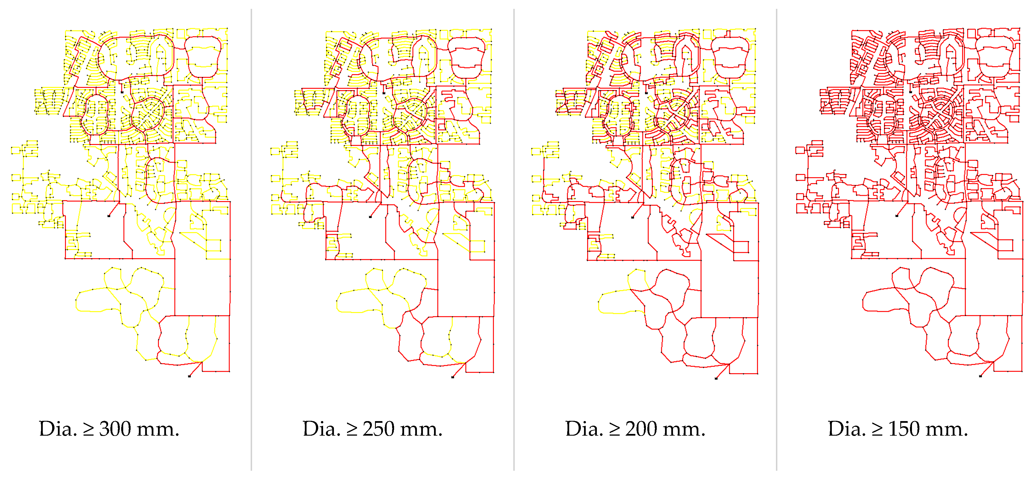
(1): A larger number of valve installations allows a constant restoration efficiency to be achieved for various instances of seismic damage.

(2): In general, one-end valve installation is regarded to be more cost-effective than installation at both ends of a pipe, as seen in the economic analysis (Table 5). The results may vary depending on the application network and locations of critical facilities and damage occurrence.

(3): For a blocked network, installing valves on main transmission lines and the boundary pipes is the most cost-effective option for damage restoration.

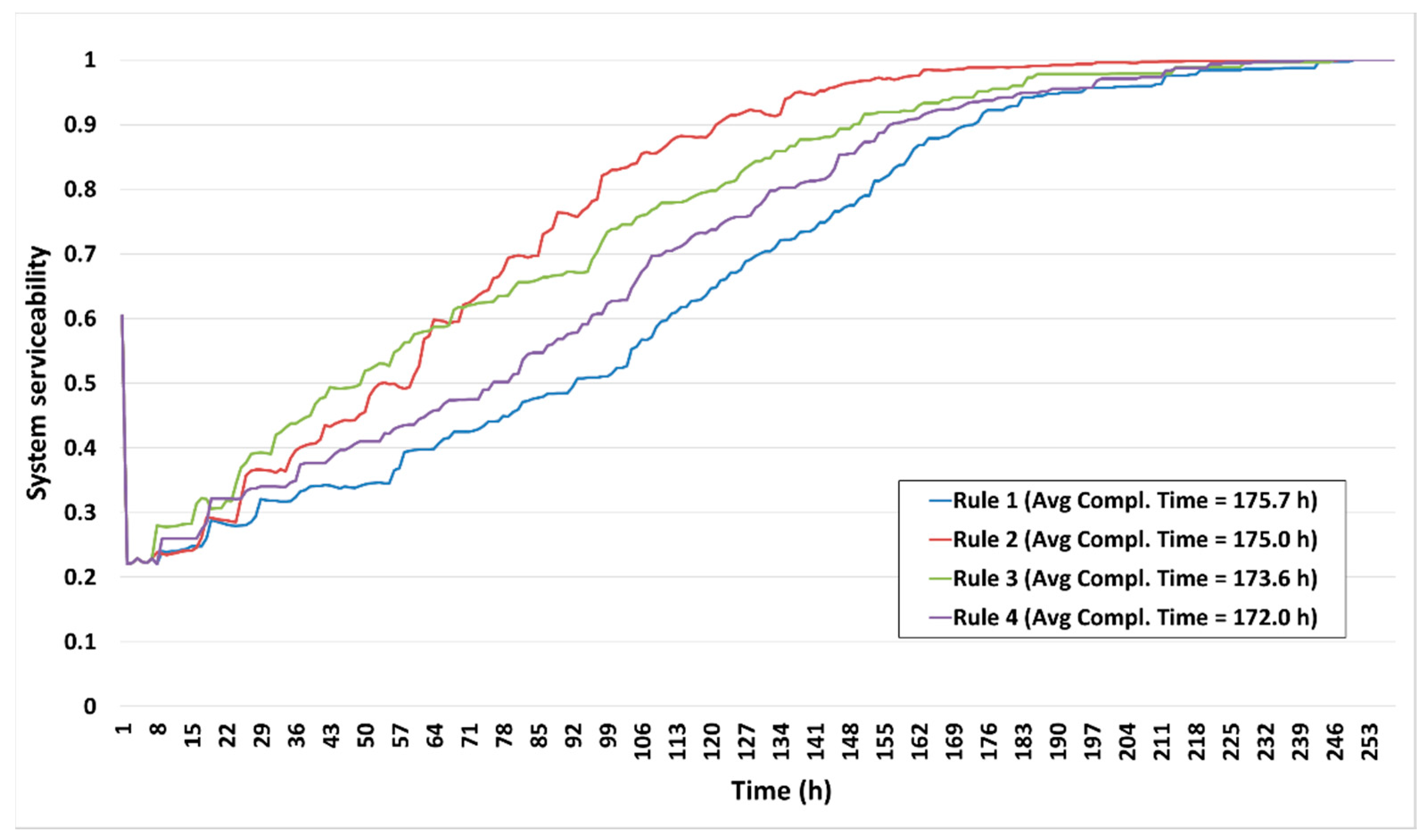
(4): The segment-based restoration rules are superior to the pipe-based restoration scheme. Among the segment-based restorations, it is more efficient to preferentially restore segments with large water suspension flows (Rule 2). In real cases, it may be more efficient to combine multiple rules rather than apply a single strategy. According to Figure 8, it would be more efficient to apply Rule 3 at the early stages and Rule 2 during later times. Here, the time for transition between the rules would be an issue. This is an interesting topic to investigate in the future.

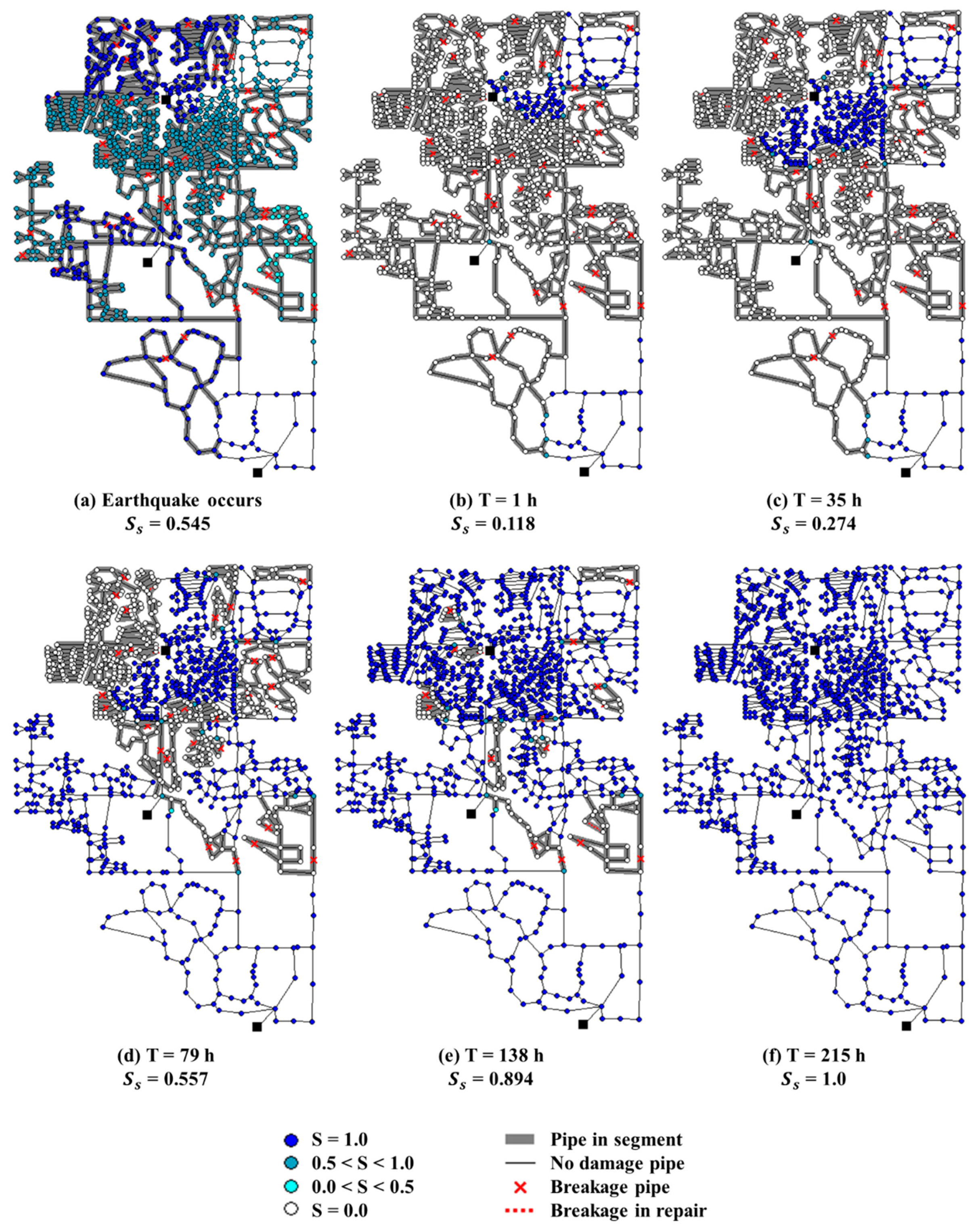
The spatio-temporal restoration progress map generated from the model can be used to identify the restoration status of the network in time and space for the assessment of the expected service suspension area, expected restoration completion time, and serviceability at individual nodes. Therefore, the model can be used as a decision-making tool for real-time operation under seismic hazard if deep knowledge about the network and data are available. The model is more applicable for the design and planning of a network against seismic damage.

As part of future research, the model will be further developed to consider not only the current emergent restoration (i.e., broken pipe replacement) but also leakage detection and leakage resolution. Furthermore, the importance of network topology and layout in system restoration should be investigated. Applying the heuristic optimization approach to suggest an optimal valve layout would be a practical application. In addition, by using a linked simulation with other lifeline systems (e.g., roads and electric power), the model will help establish a more realistic restoration plan.