Post Evaluation of Slope Cutting on Loess Slopes under Long-Term Rainfall Based on a Model Test

Abstract

The failure of treated slopes around the world, especially in China, is occurring at a noteworthy rate, resulting in an urgent requirement for post evaluation of the treated slopes; however, there is no mature technique established for post evaluation. By using a real loess slope treated by slope cutting in Shaanxi Province as the prototype, indoor geotechnical tests and model tests were performed to reveal the rainwater infiltration characteristics and pressure-varying characteristics inside the slope, the results of which were used to conduct a post evaluation of the slope in situ. The results mainly showed that the effect of rainwater scouring on the slope surface weakened gradually into a steady state at the end of the first year. The rainwater upon the slope surface preferentially infiltrated the platforms with gradually reducing rates; however, the observed wetting front cannot be regarded as the border between the unsaturated and saturated loesses. The soil pressures inside the slope did not increase, but decreased during the early period of rainfall. The displacements of key points mainly occurred during the first two years and then steady periods were entered. The above results were utilized to conduct a post evaluation of the slope prototype, by which a post evaluation framework was constructed.

1. Introduction

In the 20th century, China started to develop the western area, which promoted the construction of houses, highways, railways, etc., which inevitably brought a large number of slopes under treatment. More than 70% of western China is covered by loess, characterized by collapsibility under rainfall, which is more evident in northern Shaanxi. Thus, long-term rainfall is the most active factor influencing slope stability in western China [1]. Comparably, the failures of loess slopes after treatment has occurred widely in other areas around the world, such as that of the Zemun Loess Plateau on the northern outskirts of Belgrade in Serbia [2] and that in the loess-mantled regions of the American Midwest and Hungary [3]. Evidently, the treated loess slopes that are widespread around the world require further treatments to defend their safety. This falls under the area of slope post evaluation, which is different from the safety investigation undertaken in the design stage [4].

Addressed by scholars, slope post evaluation concerns the whole situation of the subject, including its adaptations to the environment, displacements and cracks [5,6]. To make the post evaluation of slopes more reasonable, Fang [7] adopted a rectified concept of the post evaluation and made use of an evaluation method based on stress. However, the main post evaluation theory still falls under the scope of field investigations and judgment based on experience [5,7]. The developed post evaluation theories all fall under the scope of qualitative and semiquantitative methods, which do not consider rainfall. This is a limitation of the current post evaluation techniques.

Recently, an increasing number of scholars have made efforts in the field of slope stability evaluation when the slope is under rainfall and the associated failure mechanism, including modeling tests [8,9,10,11], numerical simulations [12,13] and field monitoring [14,15]. Raj and Sengupta [16] studied the railway embankment slope failure in Malda, India, during rainfall and found that the rainfall intensity and duration were the two critical factors influencing soil slope safety. The draining of rockfill was an effective measure for strengthening the railway embankment slope stability. Zhang et al. [17] conducted a series of model tests on slopes under rainfall to reveal the hydrological mechanism for slope failures and concisely concluded that the volumetric water content response and the matrix suction response of the slopes occurred earlier than the pore water pressure response. The loess slopes failed when the volumetric water content and the matrix suction reached their maximum and minimum values, respectively; thus, a warning threshold model for the slope instability induced by rainfall was proposed. Huang et al. [18] developed a piezometer system to monitor the hydrological conditions of a highway earth slope in Taiwan under rainfall, from which it was found that the pore water pressures inside the slope were apparently pertinent to the rainfall pattern and the ground water flow. For a deep-seated slope failure, it was suggested to combine the imperatively monitored pore water pressures with the monitored stresses to establish a slope failure warning system. Perceivably, rainfall is the most critical factor influencing slope safety, causing surface erosion of slopes [19,20,21,22,23], reducing the strength of slope soils by infiltration [24,25,26] and degrading the stress situation in the slope soil as it becomes saturated [27,28,29,30,31]. Regarding a loess slope, rainwater flows can scour the slope surface easily, generating gullies and fall holes [32]. Thus, some researchers have employed a geobarrier system to defend soil slopes from rainwater-scouring and to ascertain the slope safety under rainfall [33]. It has been widely accepted that matrix suction plays an important role in the strength of the slope soil and is thus very critical to slope stability [34]. Under rainfall, rainwater infiltration leads to an increase in the water content of the slope soils, thus reducing the suction inside, which in turn causes instability of the slopes. For loess slopes incorporating more fines, this is more significant [35]. Moreover, during the rainfall process, the effective stress of the slope soil declines, which also causes a decrease in the soil strength, being adverse to the stability of the slope [36]. In summary, rainfall is a critical factor inducing slope instability. Thus, in the slope design consideration, drainage engineering is an compulsory measures.

Model tests have been used by a huge number of scholars to study slope stability and the slope failure mechanism to assess its reliability. Schenato et al. [37] employed optical fiber sensors in a model test to investigate the mechanical evolution in the slope. The results indicated the four stages of slope evolution under rainfall, from which the effectiveness of the fiber system in model tests was validated. Lan et al. [38] conducted model tests to investigate the expansion and contraction of loess slopes with moisture fluctuations, and established the relationship between the deformation of the loess slope and weather variation. Chen et al. [39] investigated the influence of the vegetation on rainwater scouring on the soil slope by model tests, and announced that the vegetation cover can adjust the rainfall patterns and alleviate rainwater splash erosion. Hung et al. [40] employed model tests to investigate the effects of earthquakes and rainfall on soil slopes. It was found that an earthquake is the factor influencing the slope stability most evidently. Sun et al. [41] used a model test to explore the influencing mechanism of rainfall on loess slopes and found that the infiltrated rainwater reduces the suction of the slope soils, causing a reduction in the shear strength of the slope loess, which eventually causes slope failure. In summary, it can be inferred that the ensuing studies of loess slopes mainly concern the pre-evaluation phase (regarding the design work), and only a very limited number of post evaluation studies have considered rainfall.

In order to facilitate the remediation of loess slopes treated in northern Shaanxi, a physical model of loess corresponding to a real slope was used to study the effects of slope-cutting treatment. The rainwater percolation and the variations in the pressures and displacements of representing positions were obtained, and they were utilized to conduct the post evaluation of the corresponding real slope. This technology of post evaluation presents an innovation for the assessment of the effects of the treatment of other types of slopes; meanwhile, the rainwater infiltration characteristics and the varying principles in the displacements and pressures of the slope may facilitate further research and design work in this regard.

2. Prototype Failure

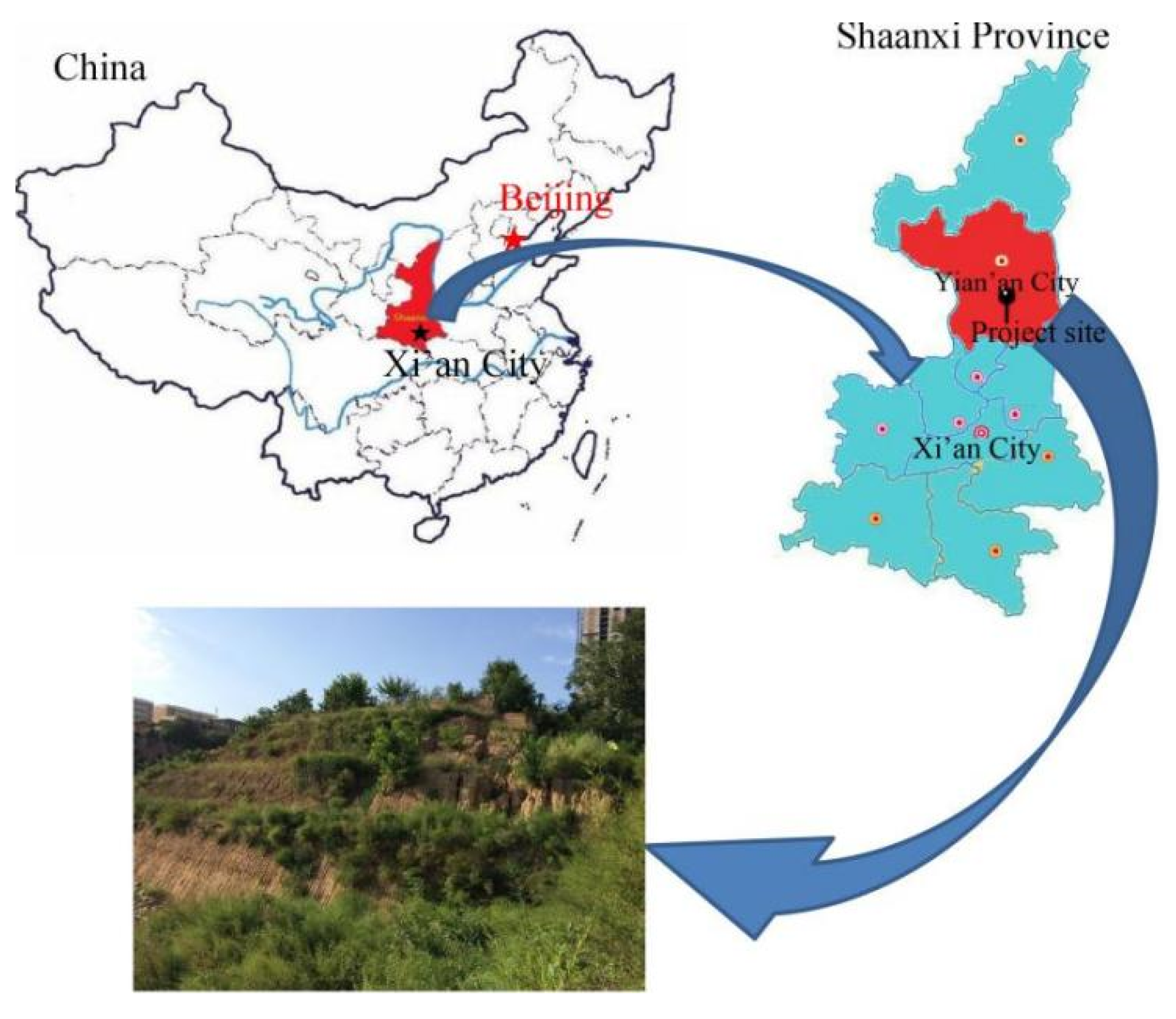
The current prototype slope is located in Luochuan County, Yan’an city, Shaanxi Province, with a latitude of 35°45′19.46″ north and a longitude of 109°25′34.63″ east, as shown in Figure 1. The elevation of Luochuan County fluctuates by approximately 1100 m. With a temperate continental monsoon climate, this area has an annual maximum temperature of 37.4 °C and an average temperature of 5~17 °C. The average precipitation of Luochuan County is approximately 606 mm per year, mainly occurring in July, August and September.

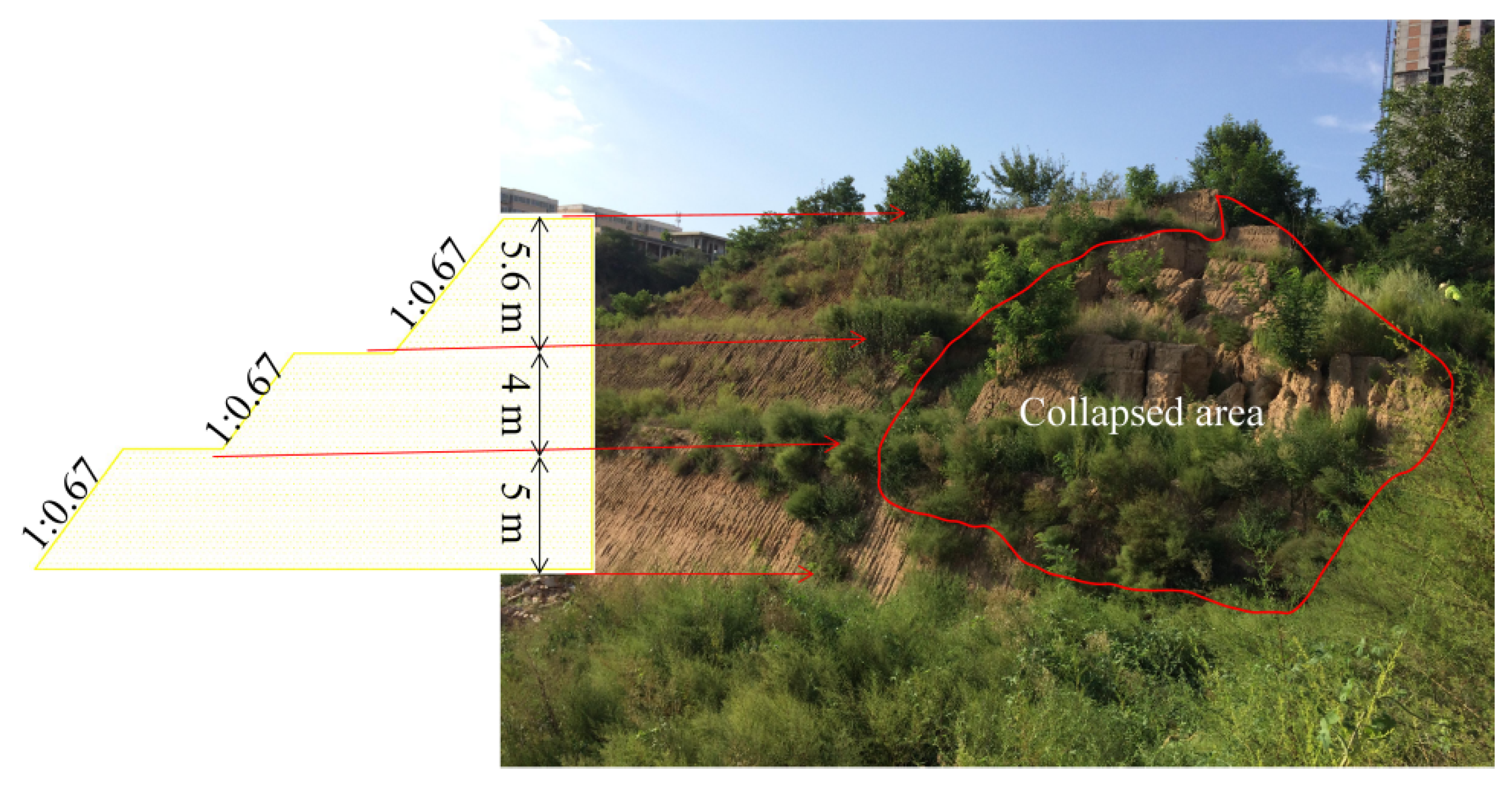
Located on the Loess Plateau, the loess slope included in this study was treated by slope cutting, and has a group of houses on the crest. From the field investigation, the slope wholly consists of loess formed in the late Pleistocene epoch. As Figure 2 illustrates, the slope prototype was 7.6 m high, and was cut into three grades of the same gradients 56°. The first grade was 5 m high, while the second and the third grades were 4 m and 5.6 m high, respectively. The widths of the second and third grade platforms were both 3.8 m, while the length of the slope was approximately 38.7 m. With the gully close to the right of the slope, the slope was excavated inward by the rainwater vented by the gully, eventually forming the collapse area (see Figure 2).

According to the field investigation performed on 20 August 2017, this project was built in approximately 2012 and ran for approximately 5 years. After a long run, affected by rainfall, the slope had main damage on its right side (see Figure 2). From the above, it can be considered that this slope prototype was composed of homogeneous loess and was in operation for a relatively short period; however, a major collapse was caused by rainwater scouring. Thus, it was reasonably chosen as a typical loess slope treated by slope cutting, which was destroyed by rainwater, as this study concentrated on the effect of rainfall on the treatment effect of loess slopes under slope cutting regardless of other factors, such as geological conditions. To conduct the post evaluation of the current loess slope through a model test, it was determined that the total simulated duration should be 5 years to be consistent with the actual running period. According to the similarity theory, the simulated time can be shrunk by 100 times, allowing the model test to be finished in a reasonable duration.

3. Methodology and Test Model

3.1. Test Device

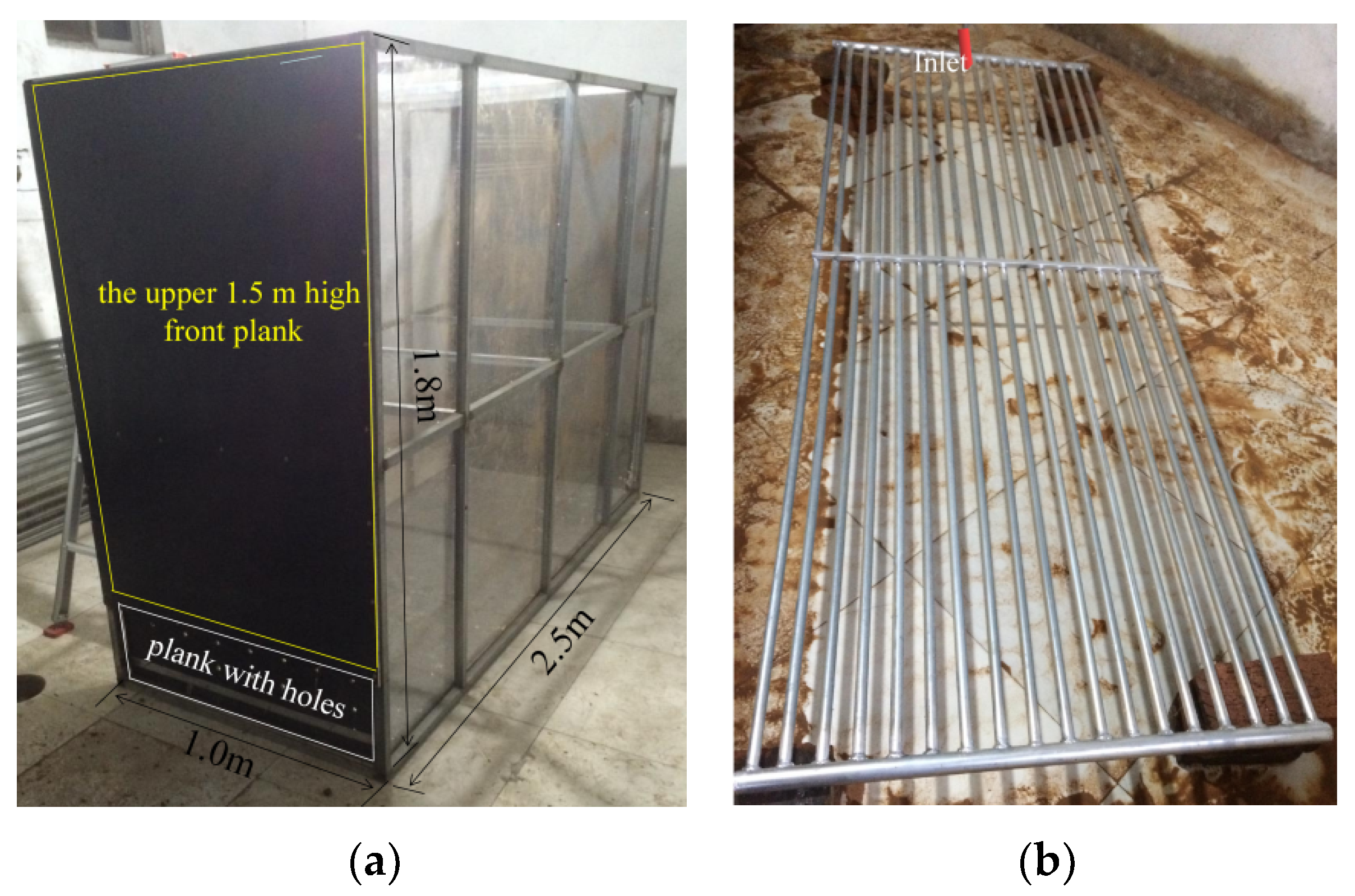
The model test was performed in the Soil Mechanics Laboratory of Shangluo University, China. From the report of Liu et al. [42], a model box with a width of 1 m, length of 2.5 m and height of 1.8 m was used in the test (see Figure 3a). The box walls of the left and right sides were made from organic glass, allowing the displacements inside the slope model to be captured by the camera. The base, front and back walls of the box were all made from planks, while the upper 1.5-m-high part of the front plank was removable, allowing the model slope surface to be free.

The rainfall simulator was a steel frame with drilled holes of 1 mm in diameter on one side. A valve connected the rainfall simulator to the water source (see Figure 3b) and adjusted the rainfall intensity. Before the start of the experiment, the simulating rainfall intensity was calibrated to a certain value according to the real rainfall, in which a beaker and measuring cylinder was adopted as the calibrator. The rainfall intensity calibration steps were as follows: (1) three beakers were placed under the rainfall simulator at different positions after the valve connecting the water pipe and the rainfall simulator was opened; (2) the three beakers were moved out five minutes later, and the water volumes contained within them were measured by the cylinder; (3) the rainfall intensities of the three positions were calculated as the corresponding water volume divided by the cross-sectional area of the beaker; (4) the average rainfall intensity was calculated from the rainfall intensities of the three positions; and (5) if the average rainfall intensity did not equal the required value, the valve opening was adjusted, and the steps above were repeated until the required rainfall intensity was achieved. Additionally, from the collected water volumes in the three beakers during the five minutes under the required rainfall intensity (31.94 mm/h), we derived that the uniformity coefficient of the rainfall simulator under a rainfall intensity of 31.94 mm/h was 0.93. This met the uniformity requirement of the model test. As the duration of each rainfall event was exactly two hours, the total rainfall amount from each rainfall event was derived as 31.94 mm/h multiplied by 2 h, resulting in a value of 63.88 mm.

3.2. Test Model

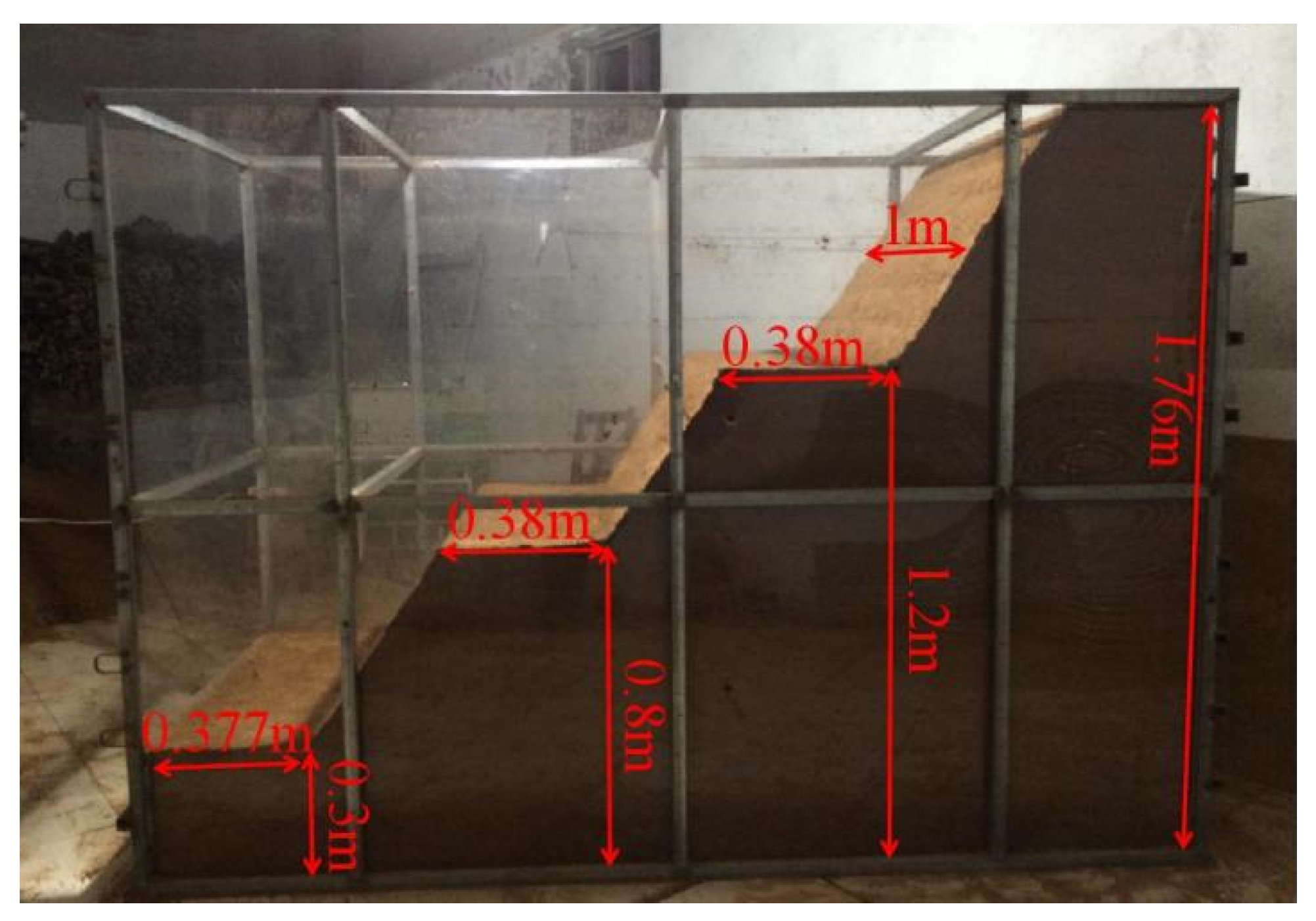
The current slope model was built to fully correspond to the prototype slope in Luochuan County, Yan’an City, Shaanxi Province, as depicted in Figure 1. With a scale of 1:10, the height of the model slope was 1.76 m, while the length of the model was 2.5 m. The three platforms of the slope model were approximately 0.38 m, while the gradients of the three grades of the slope were exactly 56°, identical to the slope prototype. In full correspondence with the slope prototype, the first, second and third grades of the slope heights were 0.5 m, 0.4 m and 0.56 m, respectively (Figure 4).

Similar to the research of Liu et al. [42], the slope in situ was first sampled by ring knife to obtain undisturbed samples, which was performed on 20 August 2017. The water content, density, permeability, grain size distribution and shear strength of the slope loess were obtained via laboratory tests. Reasonably, the loess of the model slope was collected from the site of the prototype slope. The slope model was built using the method of stratified compaction. That is, the soil was first prepared with a certain water content, and then, the loess mass of each layer of 10 cm was weighed before being used to fill the model box. As the box was filled to the certain height, the front upper plank of the model box was removed, and the filled model was cut to the dimensions corresponding to the slope prototype. Then, the constructed slope model was left standing for one year prior to the start of the rainfall experiment to simulate the formation process and the geological conditions of the slope prototype, to increase the reliability of the experimental results.

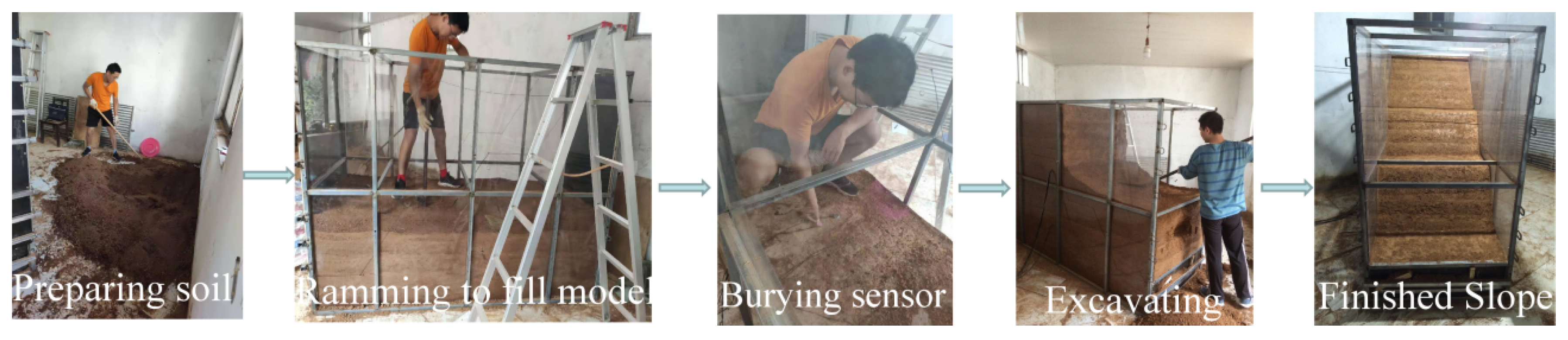
As Figure 5 shows, building the slope model was a complex process and it can be expressed by the following:

The loess obtained from the slope site was prepared such that it had an identical water content to the prototype slope (ω = 17.4%), and then, a certain mass of the prepared loess was added to the model box as a layer, which was compacted to the thickness of 10 cm.

Within the model slope building process, the soil pressure sensors and pore-water pressure sensors were buried at the prescribed positions in the model.

Synchronously, inner displacement marks were set with colored sand particles next to the two side walls of the model box, to show the displacements inside the slope model.

As the model was compacted to the required height, it was cut to the same dimensions as the prototype.

Lastly, one displacement mark was fixed at each of the three slope shoulders.

3.3. Model Materials and Similarity Relations

The model slope was wholly constructed from the loess of the prototype slope. Thus, all the hydraulic and mechanical properties of the model slope loess were identical to the properties of the prototype. The critical soil property values are listed in

Table 1. Key properties of the model soil material.

Parameters	Value	Parameters	Value
Water content (%)	1.42	Compression modulus (MPa)	5.58
Permeability coefficient (cm/s)	5.4 × 10−4	Internal friction angle (°)	27.0
Density (g/cm3)	17.4	Cohesion (kPa)	15.0

.

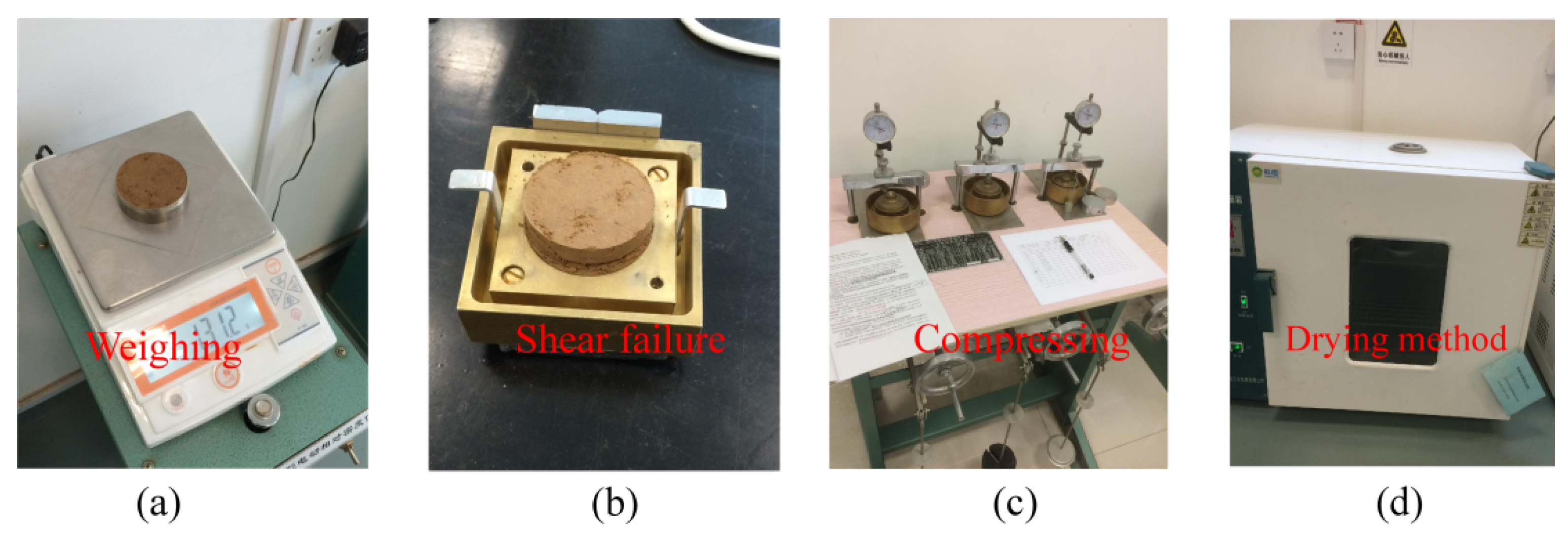
It is noteworthy that the parameters in Table 1 were obtained from geotechnical tests conducted according to Liu et al. [42]. The water content of the soil was taken from the water content experiment using the oven drying method. The permeability coefficient of the soil was obtained from the standard permeability test of varying head. The soil density was obtained from standard ring knife tests. The compression modulus of the soil was measured by the compression test. The cohesion and internal friction angle of the soil were obtained from the direct shear test of quick shear, as the quick and sudden failures of loess slopes usually happen under rainfall. For the sake of clarity, the geotechnical test process is depicted in Figure 6.

According to the π theorem [43,44], the similarity criterion of variables in model tests can be derived from the dimension analysis. As the model slope is considerably complex, it is impossible to meet the similarities of all the parameters. Thus, only the parameters of geometric dimension, gravity acceleration and density were chosen as the fundamental dimensions considering the purpose of the model test. Relevant similar constants in the test are tabulated in

Table 2. Similarity ratios of the test model.

Parameters	Similarity Relation	Similarity Constant
Geometric dimension (L)	CL	10
Density (ρ)	Cρ	1
Gravity acceleration (g)	Cg	1
Stress (σ)	Cσ = CρCgCL	10
Strain (ε)	Cε = 1	1
Displacement (s)	Cs = CL	10
Cohesion (C)	CC = CρCgCL	10
Internal friction angle (φ)	Cφ = 1	1
Rainfall intensity (Cq)	Cq = Cρ0Cg0.5CL0.5	$\sqrt{10}$

.

It is noteworthy that the similarity constant of the rainfall time was derived from a calculation according to Terzaghi’s consolidation theorem [45] but not from the π theorem. This method was validated by Butterfield [46] and Garnier et al. [47] and was employed by Tang [48] in studies of the slope stability with rainfall. Though the size of the slope model was different from that of the slope in situ, the consolidation degrees of the slope model and the slope in situ should be identical in the testing process. According to Terzaghi’s consolidation principle, the consolidation degree of the slope soils can be expressed as

$$U=1-\beta .e^{-\lambda .T_V}$$

(1)

Here, β and λ are the invariable constants and T_v is the time, which only varies with the time elapsed. Therefore, the consolidation degree U varies only with time t.

Reasonably, the parameters β and λ of the slope model and the slope prototype have the same value. Therefore, under the identical consolidation degree, the slope model has the same time factors with the slope prototype, i.e.,

$$T_{Vp}=T_{Vm}$$

(2)

Here, T_Vm and T_Vp are the time factors of the slope model and the slope prototype, respectively. Equations (3) and (4) depict the relationships between the time factors and the consolidation time.

$$t_p=\left(H_p{}^2/C_V\right)T_{Vp}$$

(3)

$$t_m=\left(H_m{}^2/C_V\right)T_{Vm}$$

(4)

Here, t_m is the consolidation time of the model slope and t_p is that of the the prototype slope; H_m and H_p denote the sizes of the model slope and the prototype slope, respectively; and C_v denotes the same consolidation constant of the model slope and the prototype slope. Therefore, we can derive the similarity constant of the rainfall time as

$$C_t=\frac{t_p}{t_m}=\frac{H_p^2}{H_m^2}=C_L^2$$

(5)

Accordingly, C_L was 10 here; thus, C_t was derived as 100. As a result, the experimental time was shrunk by 100 times, allowing the experiment to be completed in a shorter period. According to the field investigation, the slope prototype had been in operation for approximately five years. Thus the experimental time was 0.05 years in this study.

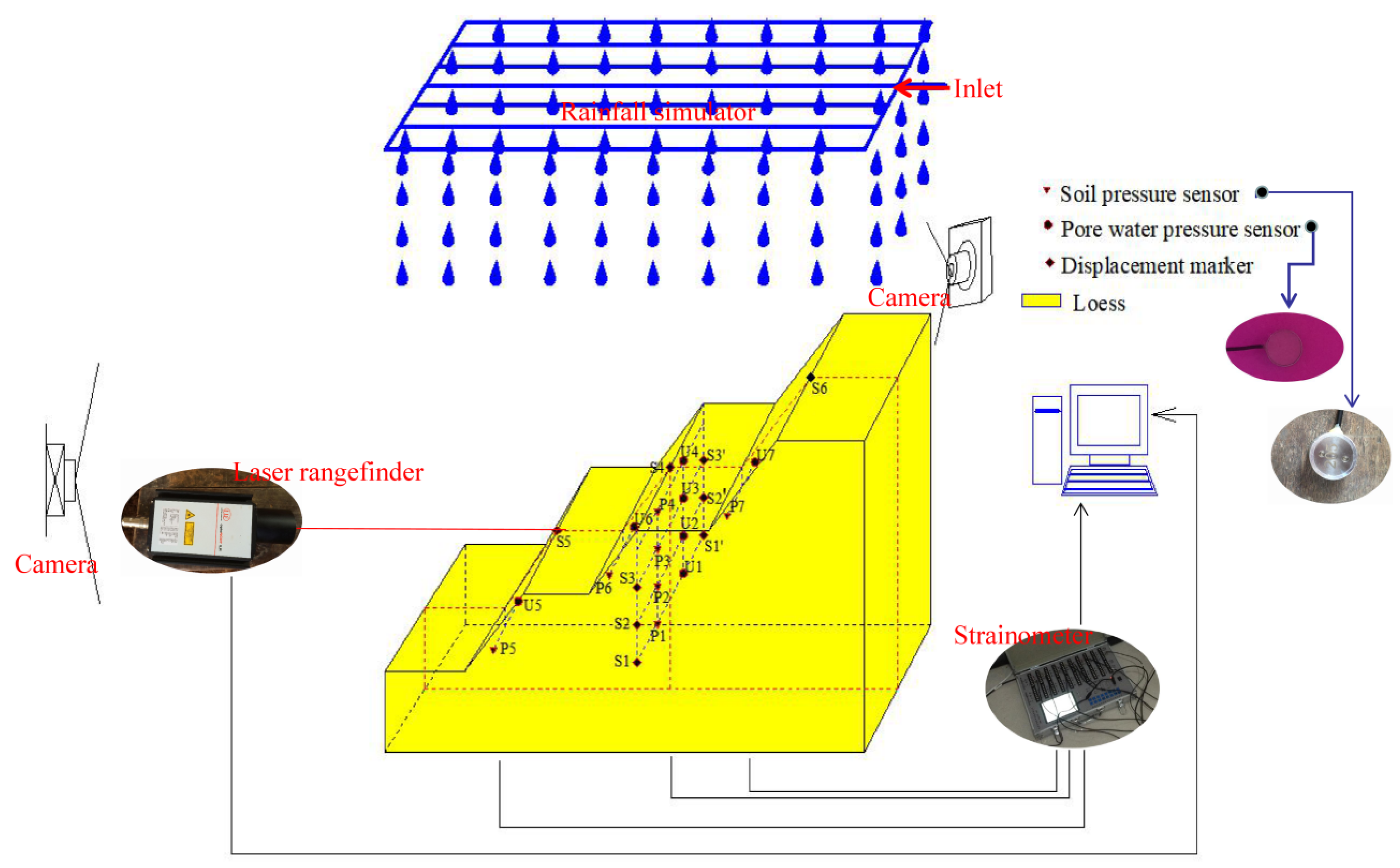
3.4. Measuring System and Rainfall Scheme

In total, the model test employed seven pore pressure sensors and seven soil pressure sensors. The pore pressure sensor U4 was seated at a position 10 cm under the shoulder of the second grade of the model slope, and the seated depth of U3, U2, and U1 increased by 20 cm sequentially in a perpendicular line from U4. The pore pressure sensors U5, U6 and U7 were seated 10 cm under the slope toes of the first, second and third grades, respectively. To facilitate meaningful results, the soil pressure sensors P1, P2, P3, P4, P5, P6 and P7 were buried at identical positions with those of U1, U2, U3, U4, U5, U6 and U7, respectively. A strainometer was connected to the pressure sensors, and converted the pressures into digital signals for the computer to store. Although the model test analyzed a planar problem, the pressure sensors were seated close the axial plane of the model to deliver more reliable data [42].

Three displacement marks were set at the three slope shoulders, which are shown in Figure 7 as S5, S4, and S6 at the first, second and third grades of slope shoulder, respectively. Three points were marked by colored sand particles close to the right wall of the model box to measure the inner displacements of the model slope, which were S1, S2, and S3. Similarly, three displacement marks, S1′, S2′ and S3′, were set by colored sand particles close to the left wall of the model box, corresponding to the positions of S1, S2 and S3. To obtain meaningful data, the depths of S1 (S1′), S2 (S2′) and S3 (S3′) were the same as those of P1, P2 and P3, respectively, as shown in Figure 7. The displacements of the marked positions were defined as the distance differences before and during rainfall, which were measured by a laser rangefinder fixed in front of the model slope. A computer connected to the laser rangefinder was used to display the distance data. It is noteworthy that the accurate displacement of S1 was the average displacements of S1 and S1′, and the same applies for S2 and S3.

At constant time intervals, photos were taken from the front and two sides of the model; thus, we obtained the rainwater infiltration process and the deformation process of the model slope during rainfall.

As addressed above, the precipitation in Luochuan County mainly happens in July, August and September, with a total amount of approximately 606 mm per year. For this study, we assumed that the annual precipitation was spread over three months, with each month only having one rainfall event of 2 h. In the remaining period of the month after the rainfall, the model slope stayed undisturbed. Thus, the rainfall intensity in situ was calculated as being 101 mm/h constantly. The simulated rainfall intensity was derived as 101 mm/h divided by the similarity constant $\sqrt{10}$, resulting in a value of 31.94 mm/h. In the same way, the total experimental time was derived as five years divided by the similarity constant 100 (see Equation (5)), producing a value of 0.05 years, i.e., 18 days. The time intervals between each of the 3 simulated rainfall events were derived as 30 days divided by the similarity constant 100, and then 2 h were subtracted, producing a period of 5.2 h. The testing scheme of one year is detailed in

Table 3. Model test scheme (the scheme in this table was repeated 5 times to simulate 5 years of rainfall).

Simulated Time	Actual Time	Rainfall Start	Rainfall End	Read Data
0 h	0 h	Yes		Yes
2 h	2 h		Yes	Yes
7.2 h	30 d	Yes		Yes
7.2 h + 2 h	30 d + 2 h		Yes	Yes
14.4 h	60 d	Yes		Yes
14.4 h + 2 h	60 d + 2 h		Yes	Yes
21.6 h	90 d			Yes
28.8 h	120 d			Yes
36 h	150 d			Yes
43.2 h	180 d			Yes
50.4 h	210 d			Yes
57.6 h	240 d			Yes
64.8 h	270 d			Yes
72 h	300 d			Yes
79.2 h	330 d			Yes
86.4 h	360 d			Yes

, and this was repeated 5 times to accomplish the rainfall of 5 years.

In general, the experimental steps can be depicted as follows:

Before burying the pressure sensors in the model construction process, their original values were measured.

As the construction of the slope model was completed, the pressure sensor cables were attached to the strainometer, which was used to send the pressure data to the computer. Additionally, a laser rangefinder seated in front of the slope model was connected to the computer to obtain the distances between the fixed position and the displacement marks (S1, S1′, S2, S2′, S3, S3′, S4, S5, S6), thus deriving the horizontal displacements of the key points.

The rainfall intensity of the rainfall simulator was adjusted to 31.94 mm/h, and acted the rainfall simulator on the model slope while the computer program used for data-capture started.

The scheme in Table 3 was repeated 5 times to accomplish five years of rainfall simulation, as the computer recorded the data of the pore water pressures, soil pressures and horizontal displacements of the key points.

3.5. Compound Safety Factor Calculation

In the field of geotechnical engineering, safety factors have been widely accepted as indicators of the safety situations of slopes. As Equation (6) shows, the slope safety factor can be expressed as the ratio of the total anti-slide moment to the total sliding moment.

$$K=\frac{{\displaystyle \sum M_{resisting}}}{{\displaystyle \sum M_{sliding}}}$$

(6)

Here, M_resisting is the anti-slide moment at a slice base within the sliding body, and M_sliding is the sliding moment at the slice base. Within the limited equilibrium method, the sliding surface is occasionally assumed as an arc. In this situation, the arm of a moment is identical to the arc radius, and the interslice forces are totally excluded from the calculation. Adopting this consideration, the slope safety factor was simplified as

$$K=\frac{{\displaystyle \sum F_{resisting}}}{{\displaystyle \sum F_{sliding}}}$$

(7)

Here, F_resisting is the anti-slide force at the slice base, while F_sliding is the sliding force at the slice base. Taking the suction in the slope soils into consideration, Wang and Zhang [49] reconstructed the anti-slide force and the sliding force equations of the slice as

$$F_{resisting}=W_i\cos {\alpha }_i\tan \phi +\frac{\left(u_s\tan {\phi }^b+c\right)B}{\cos {\alpha }_i}$$

(8)

$$F_{sliding}=W_i\sin {\alpha }_i$$

(9)

Accordingly, W_i and α_i are the weight and bottom inclination angle of sliding slice i, respectively; c and φ are the cohesion and internal friction angle at the bottom of sliding slice i, respectively; u_s and φ^b are the matrix suction and suction friction angle at the bottom of sliding slice i, respectively; φ^b usually has a value around φ/2, according to Fredlund and Rahardjo [50]; and B denotes the sliding slice width. If the vertical soil pressure σ_y at the bottom of the sliding slice can be obtained from the model test, W_i can be calculated by

$$W_i={\sigma }_y\cdot B$$

(10)

Substituting Equation (10) into Equations (8) and (9), the results of which were then substituted into Equation (7), a new equation of the safety factor was constructed as

$$K=\frac{{\displaystyle \sum \left[{\sigma }_{y}B\cos {\alpha }_i\tan \phi +\frac{\left(u_s\tan {\phi }^b+c\right)B}{\cos {\alpha }_i}\right]}}{{\displaystyle \sum \left[{\sigma }_{y}B\sin {\alpha }_i\right]}}$$

(11)

Using Equation (11) to calculate the slope safety factors, the sliding body should first be divided into vertical slices. Then, assuming that the positions with the same burial depth had identical soil pressures and matrix suction, the soil pressures and suction at the bottoms of the slices can be obtained from the model test data. In most cases, the interpolation method could be an useful tool in the determination of the pressures and suction of the slice bottoms from adjacent points.

4. Results and Discussion

4.1. Slope Scour Failure Process

The camera seated in front of the model box was used to capture the scouring process of the model slope at certain time intervals. In accordance with the field investigation, the simulation period was five years, corresponding to five rounds of rainfall. Nevertheless, this section does not present the rainfall scouring process on the model slope due to its negligibility.

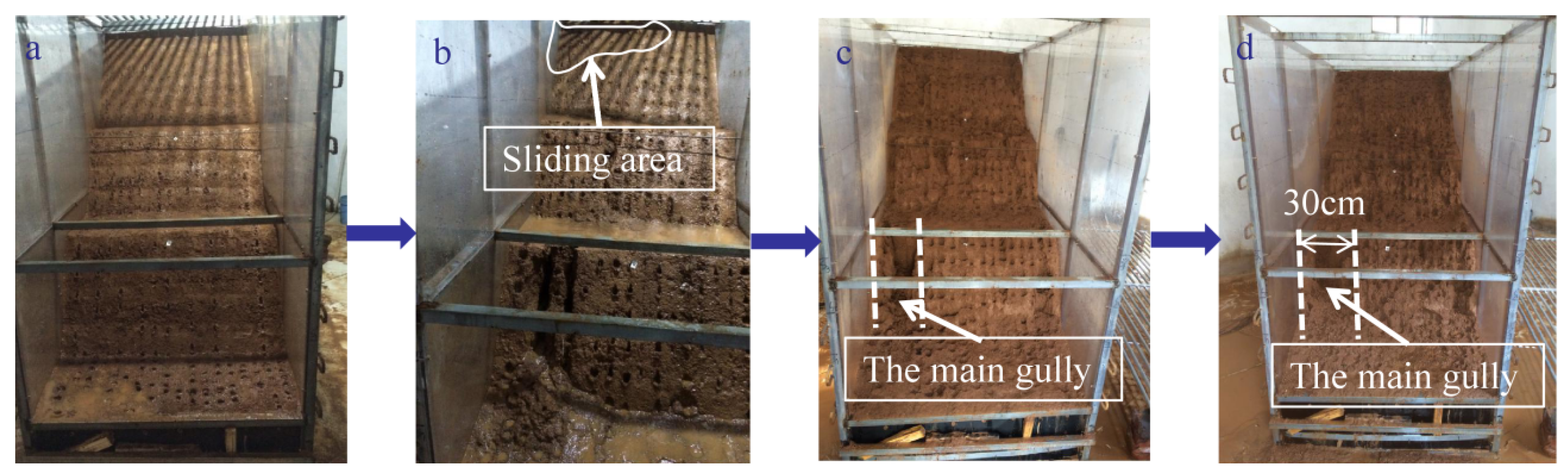
Figure 8 presents the scouring process of the slope model during rainfall. Evidently, the scouring effect in the first round was very significant. Within 25 min from the beginning of the first rainfall, the scour was reasonably categorized as splash erosion, as the raindrops impacted the slope surface and made shallow pits. Later on, from 25 min to 60 min, the scour form transformed into surface erosion. While the first rainfall progressed for 25 min, the formed shallow pits gradually connected, inducing shallow gullies. At 45 min from the start of the rainfall, a shallow sliding of a small size occurred on the left portion of the top grade of the model slope. Meanwhile, gullies on the model slope were completely formed. Lastly, in the period from 60 to 120 min, the scour pattern was found to constitute gully erosion and sliding. At 60 min from the start of the first rainfall, the left portion of the first slope grade developed a deep gully with a depth of 7~8 cm and a width of 5 cm, while the second slope grade showed a gully with a depth of 4~5 cm and a width of 3~4 cm. Meanwhile, larger slides happened on the middle portion of the third grade of the model slope, and ruined displacement mark S6. Understandably, the rainwater pooled on the left portion of the platform of second grade, softened the soil beneath it and promoted gully development there, which was inevitable for a loess slope under rainfall. Additionally, it was observed that the larger scale of slides on the third grade of the slope model was induced by rainwater pooled on the slope crest, which softened the loess there while percolating. In the later phase of the first rainfall, the developed gullies were widened and deepened by the downflow of the rainwater. When the first round of the first rainfall event ended, the main gully in the left part of the first slope grade was approximately 30 cm deep and 10 cm wide, as shown in Figure 9a.

As Figure 8 shows, different to the first rainfall event, the scour process of the second rainfall event consisted of only two phases, namely the undisturbed phase and the gully erosion with sliding phase. The period from the start of the rainfall to 20 min of rainfall comprised the undisturbed phase, which resulted in no perceivable surface erosion to the model slope, as the rainwater downflow was weak. Understandably, the loess within the shallow layer of the model slope consolidated in the interval between the two rainfall events, making further erosion difficult, which induced an undisturbed phase later in the process. As the rainfall continued, the shallow layer of loess softened again, inciting gully erosion with a sliding phase. The gully erosion with a sliding phase occurred in the period after 20 min of rainfall, where gullies developed and slides happened occasionally. Small scales of shallow slides occurred on the second grade of the model slope at 30 min, 40 min, 56 min and 78 min from the start of the second rainfall event, which fully ruined displacement mark S4. In the meantime, larger scales of slides occurred on the third grade of the model slope at 80 min and 100 min from the start of the second rainfall event, inducing the declination of the gradient of the third grade of the model slope. Evidently, different from first rainfall event, the slope slides in the second rainfall event had initiation stages compromising the duration of approximately the first 20 min of rainfall. As the rainfall progressed, the deeper layers of loess was wetted by the infiltrating rainwater, which caused declines in the matrix suctions, the cohesion and the frictional angles of the deeper loess. It is proven that the matrix suctions, the cohesion and the frictional angles have positive contributions to the soil shearing strength, which is the critical factor in slope safety. Thus, the decline in matrix suctions caused larger slope failures during the second rainfall event. Additionally, the dimensions and number of gullies also increased in this phase. When this rainfall event was over, the main gully at the left of the first grade of the model slope was approximately 13 cm wide, which can be seen in Figure 9a.

Compared with the previous rainfall event, the scour effect in the first round of the third rainfall event was weaker, with a small scale of shallow slides occurring on the third grade of the slope at 85 min from the start of this rainfall, and the gullies evolved gradually. It was found that, the width of the main gully in the left portion of the first grade of the slope was approximately 15 cm when this rainfall event was over.

It was found that, during the second and third rounds of rainfall, the model slope was in a relatively steady state, with no slides resulting from the weak rainwater downflow. Nevertheless, the main gully to the first slope grade persistently evolved. At the end of the third round of rainfall, the width was approximately 30 cm, and the depth was approximately 45 cm. On the one hand, the first round of rainfall formed the outlet on the slope model surface, and alleviated the scour effect of the rainfall upon the model slope. On the other hand, the consolidation of the shallow layer of the model slope within the interval between the first and the second round of rainfall impeded further scour from the rainfall. It could be reasonably concluded that the loess model slope entered a relatively steady scour stage at the beginning of the second round of rainfall, while the gully persistently evolved.

It is noteworthy that there was no sinkhole formation caused by the rainwater during the five rounds of rainfall, which should be due to the absence of a perforated crack. As engineering practice revealed, sinkholes in loess slopes are developed from perforated cracks, which form the preferential paths for venting rainwater. While the rainwater flowed through the perforated cracks, the walls of the cracks were scoured, which gradually formed sinkholes in the loess slope. Referring to the slope prototype, we can infer that a sinkhole could not form in the absence of a perforated crack in this model slope.

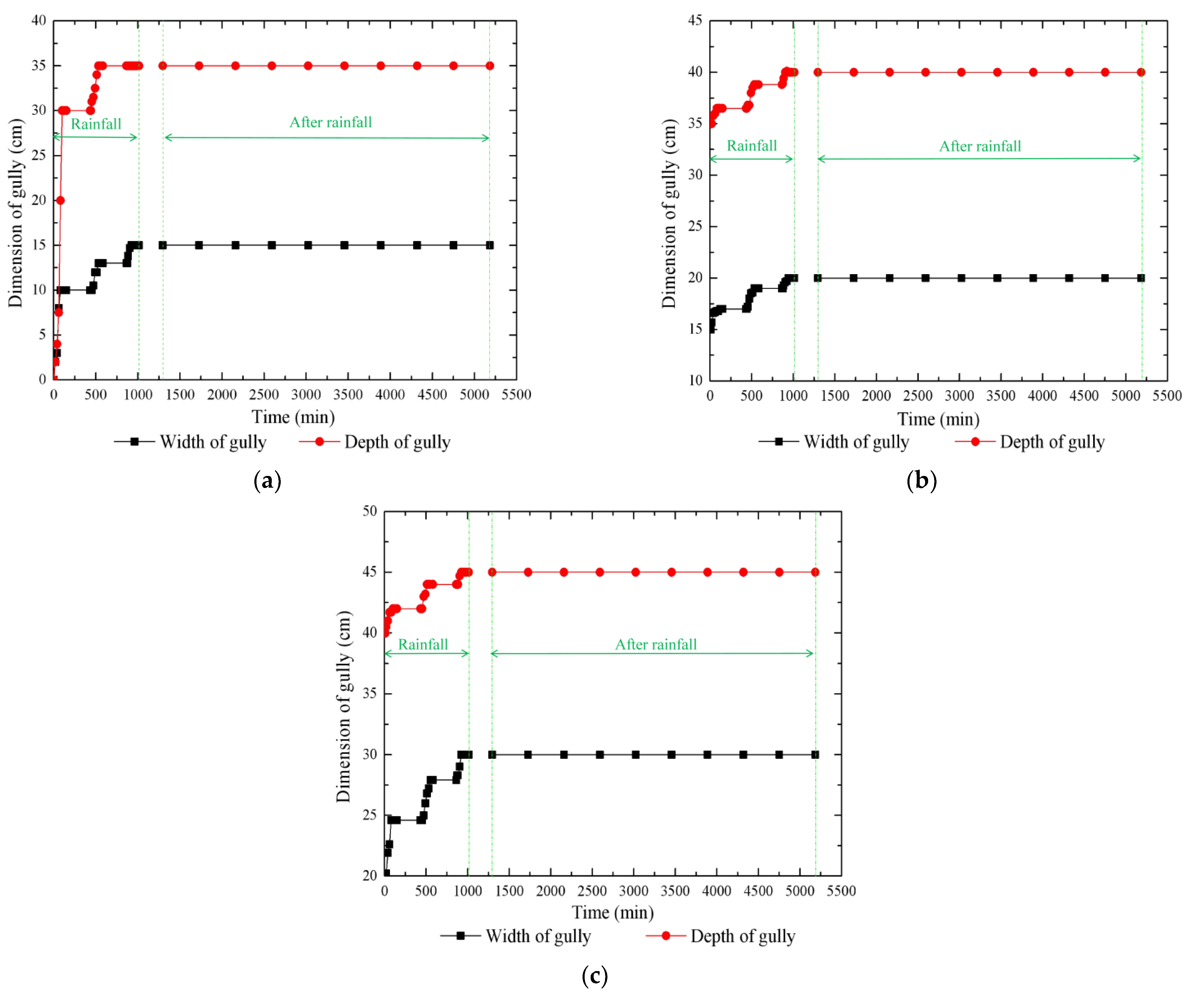
Figure 9 presents the dimension development of the main gully on the first grade of the slope within the first, second and third rounds of rainfall. As the dimension of this main gully showed no visible change after the third round, its development thereafter is not presented here. Obviously, the development of the dimensions of this main gully was most significant during the first round, particularly in the first round of the first rainfall event. The depth of this gully increased from 0 cm to 30 cm during the first round of the first rainfall and developed to 35 cm by the end of the first round of rainfall. The width of this gully increased from 0 cm to 10 cm during the first round of the first rainfall and developed to 15 cm by the end of the first round. In the following two rounds of rainfall, the dimensions of this main gully developed more slowly, particularly in regard to its depth. The depth of this gully only increased by 5 cm in both the second and third rounds. Comparably, the width of this gully increased by 5 cm and 10 cm in the second and third rounds, respectively. In summary, the development of the dimensions of the main gully on the first slope grade was the most significant, particularly in the first round of the first rainfall event, and gradually slowed over time. In the rounds after the third round, the gully dimensions showed no visible development and thus are not presented here. This could be mainly attributed to the consolidation effect of the slope soils in the intervals between rainfall events.

4.2. Rainwater Infiltration Characteristics

Rainwater percolates slope soils, inducing a higher pore water pressures in the slope, thus greatly influencing the slope stability. On the one hand, the percolated rainwater can lower the shear strength of the slope soils, which is not beneficial for treatment projects. On the other hand, the percolated rainwater can lead to large water pressures in the slope soils, which is also adverse for the safety of the slope. Scholars have investigated the effects of rainfall on slope safety and concluded that rainfall is the critical factor influencing the stability of slopes and that rainwater percolation controls the deformation processes of slopes [51,52]. In the current study, the model box sidewalls were made from transparent glass. Therefore, the camera could capture the wetting front advancing process from the sides.

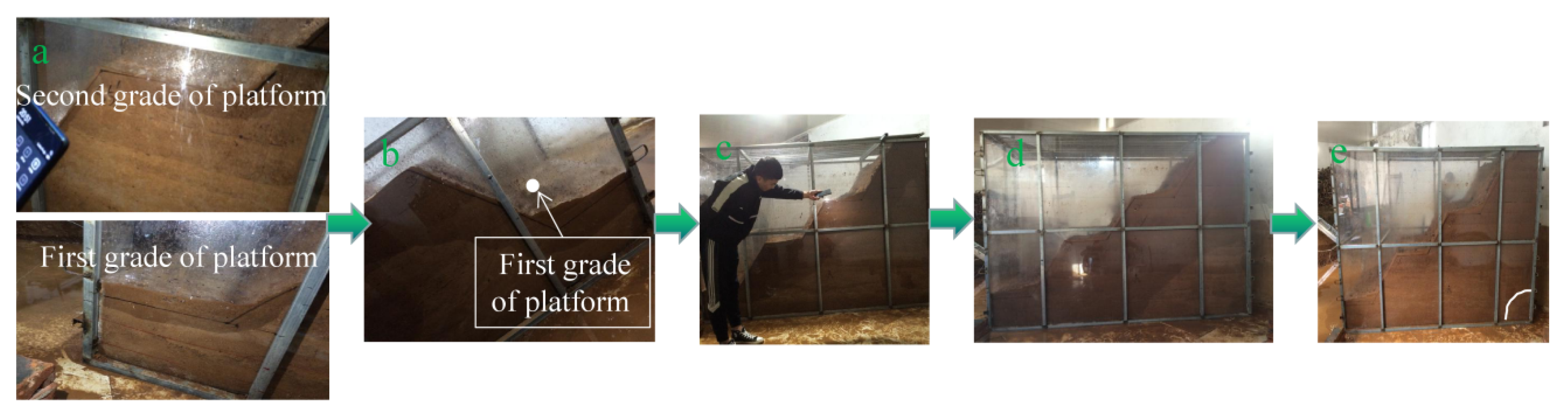
Figure 10 shows the advancing process of the wetting front in the rainfall rounds. Evidently, the rainwater percolated into the platforms preferentially, which may have been caused by rainwater pooled on the platforms. The water pooled on the platforms generated water heads there, which actuated the water into the platforms with large rates. After 10 min of the first rainfall, the percolation depths beneath the three platforms were identical at 8 cm. After 20 min of the first rainfall, the percolation depths under the first, second and third grade of the platform were 9 cm, 11 cm and 10 cm, respectively. After 40 min of the first rainfall, the percolation depths beneath the first, second and third grade of the platform were 11.3 cm, 11.5 cm and 12 cm, respectively. Therefore, it can be derived that the percolation rate of the rainwater declined with the progression of rainfall. The average percolation rate was approximately 0.8 cm/min within the first 10 min of rainfall, decreased to approximately 0.2 cm/min after 20 min of the first rainfall, and then decreased to approximately 0.075 cm/min after 40 min of the first rainfall. The pores of the unsaturated soils are partly filled with air and water. Under rainfall conditions, the rainwater must discharge the pore air to percolate into the slope soils. In the shallow layers of slope soils, the pore air was easier to be discharged, and thus showed a higher permeability; therefore, it showed a larger percolation rate at the beginning of the rainfall event, which decreased gradually with the progress of the rainfall event. Eventually, by the end of the first rainfall event, after 120 min, the average vertical percolation rate declined to approximately 0.090 cm/min. In summary, the advancement rate of the wetting front declined gradually within the first round of the first rainfall event, and eventually stabilized at 0.090 cm/min.

Additionally, the wetting front advancement rates after rainfall could be derived in the same way. Thirty minutes after the first rainfall event, the average advancement rate of the wetting fronts under the platforms was approximately 0.07 cm/min. Three hundred and twelve minutes after the first rainfall event, the percolation depths under the first, second and third grades of the platform were 25 cm, 36 cm and 38 cm, respectively, resulting in an average wetting front advancement rate of approximately 0.026 cm/min. Therefore, the wetting front advancement rates after rainfall were less than those during rainfall, with a declining trend over time. Furthermore, it can be seen from Figure 10b that the percolation depths beneath the slope shoulders were greater than those under the platforms and slope surfaces. This may have resulted from the combined influences of the percolation from the platforms and the slope surfaces, reasonably viewed as the superposition of the two influences.

Within the first round of the next two rainfall events, the wetting front persistently migrated downward at a rate lower than that during the first rainfall event, which decreased gently with time. When the third rainfall event was over, the mean advancement rate of the wetting front was approximately 0.05 cm/min. Moreover, when the rainfall events ceased, the wetting front was clear, but this became vague 5.2 h later (see Figure 11c). Five hours and twelve minutes after the second rainfall of this round, the wetting front was circular, which corresponded to the Swedish arc method for evaluating slope stability. Ultimately, 70 h after the first round of rainfall, most of the slope soils were soaked, while the lower-right triangular corner remained dry; the horizontal side of the dry area was approximately 1.3 m long.

The entire slope body was wetted 5.2 h after the second rainfall event in the third round; thus, the subsequent rainwater movement in the slope soils was not detectable. However, the shrink rate of the triangular dry area was very minor, and was even imperceptible, during the rainfall progress, at approximately 0.003 cm/min, 5.2 h after the third round of the second rain event, which is nearly 10 times lower than the shrink rate at the end of the first round.

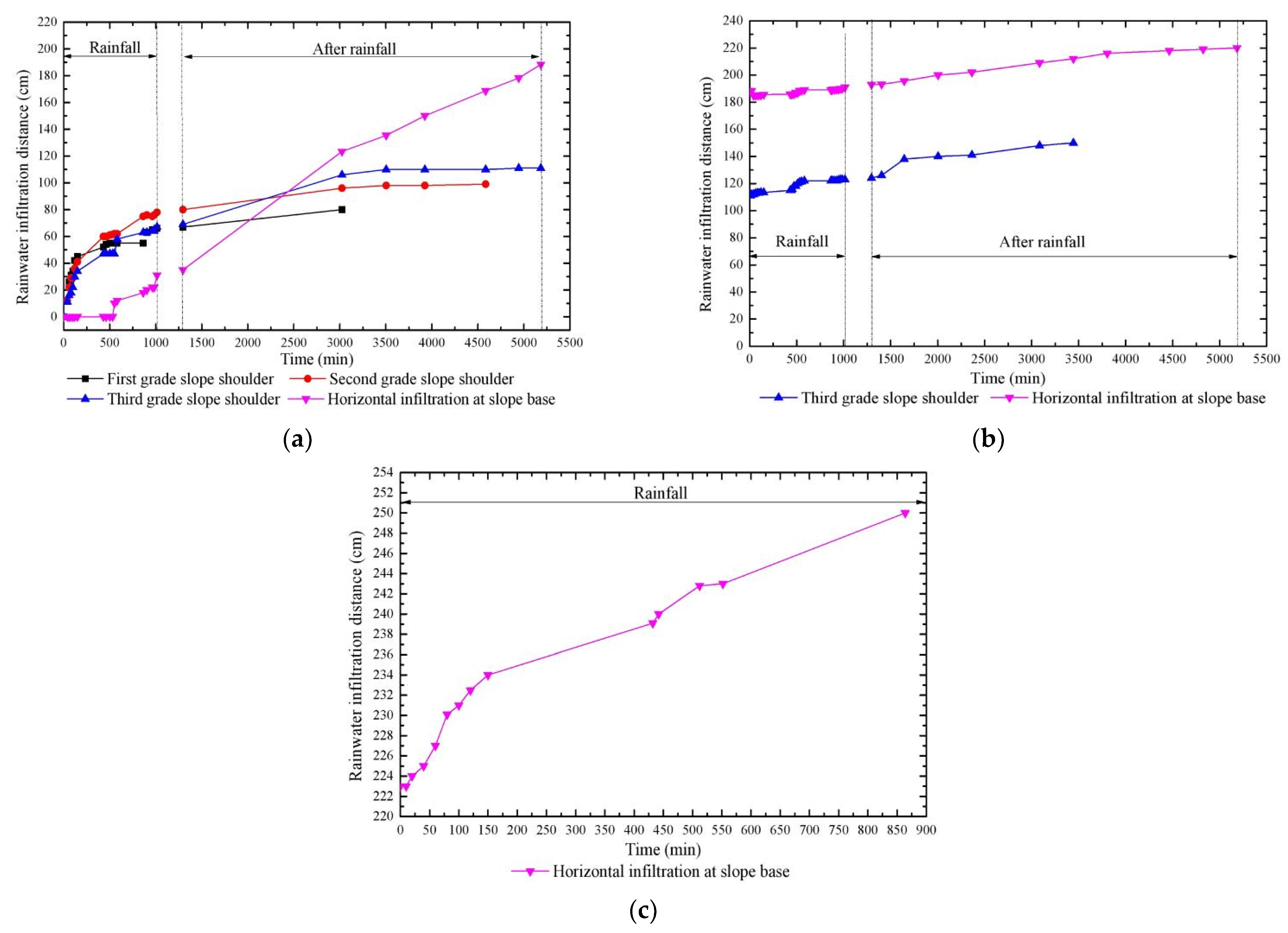
Figure 11 presents the vertical infiltration distances under the three slope shoulders and the horizontal infiltration distance at the slope base over time. It is evident that the vertical infiltration distances under the slope shoulders increased sharply in the first round, particularly during rainfall. However, the increasing rates of the vertical infiltration distances gradually decreased over time. Forty-one hours after the second round of the third rainfall event, rainwater infiltrated the slope base beneath the third grade slope shoulder, while the vertical infiltration rate decreased to approximately 0.0056 cm/min. Thus, the vertical infiltration under the slope shoulders after that time was not presented. Similarly, the horizontal infiltration caused by the migration of the rainwater accumulated near the first grade slope toe with a gradually decreasing rate. The difference being that the horizontal infiltration at the base of the slope had an initiation stage, which occurred during the 500 min after the start of the first round of rainfall. It is most noteworthy that the horizontal infiltration rate was obviously higher than the vertical infiltration rates under the slope shoulders. From Figure 11a, the average vertical infiltration rate under the slope shoulders was approximately 0.021 cm/min, while the average horizontal infiltration rate at the base of the slope was approximately 0.036 cm/min. This could be due to the structure of the horizontal layer of the slope model formed in the construction process, which provided a larger horizontal permeability compared with the vertical permeability.

4.3. Pressure Variations of the Model Slope

The slope safety mainly depends on the internal pressures, including the soil pressures and the pore water pressures. Generally, during the rainfall event, only the top layer of the slope soils was evidently penetrated by the rainwater, causing an increase in the unit weight of the top layer. As the rise of the pore water pressure in the deep layer was very limited, the increase in the soil pressure there inevitably outweighed the pore water pressure, which in turn caused an increase in the shear stress. Moreover, the limit increase in the pore water pressures could have caused the significant drop in the shear strength. In a case where the shear stress increased to the limit value, the slope would begin to fail [53]. In the current research, prior to the rainfall test, a pressure coefficient was set for each of the pressure sensors in the computer program. The program automatically converted the signals delivered by the sensors into pressures. Lastly, they were subtracted by the initial pressures to obtain the actual pressure values.

4.3.1. Pore Water Pressure Variations

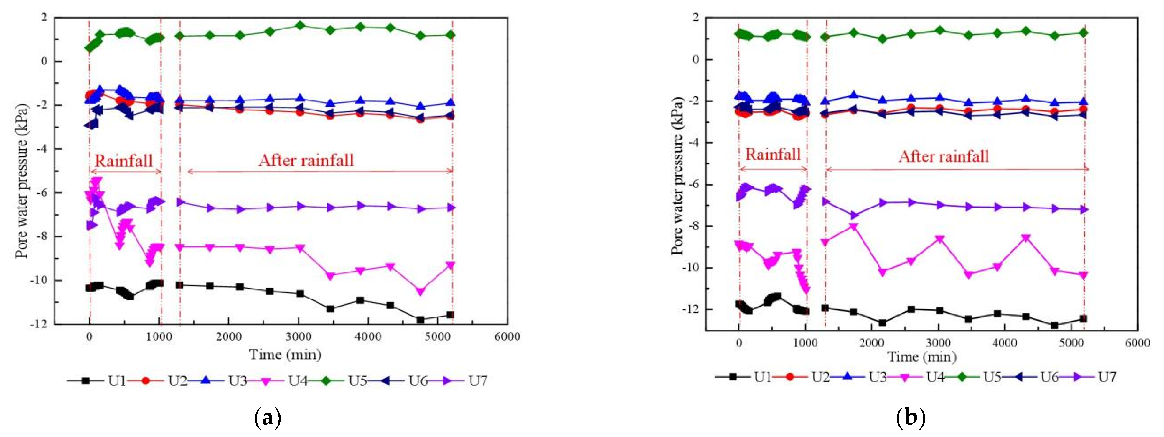
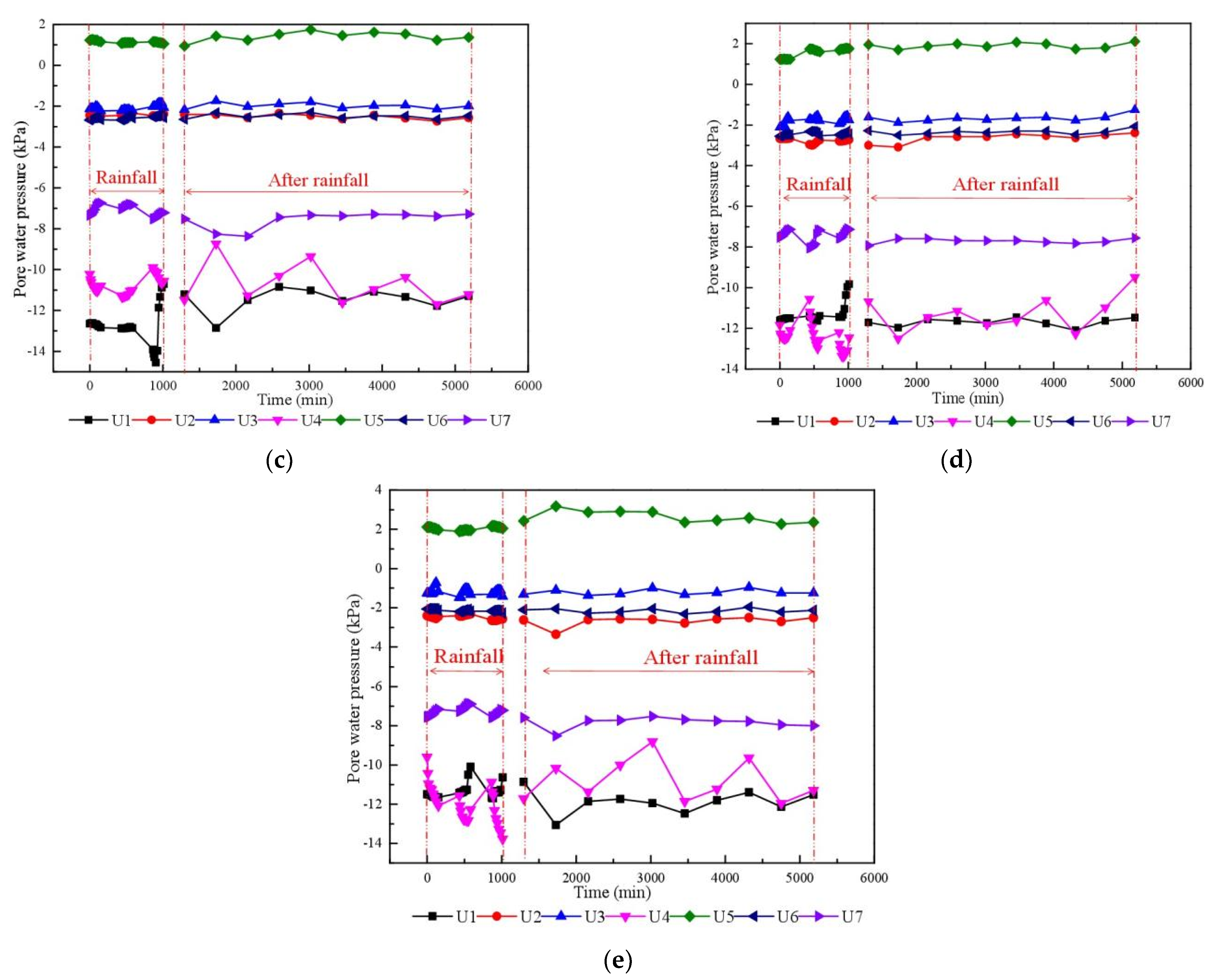
The pore water pressure variations of the seven points (U1, U2, U3, U4, U5, U6 and U7) over time are presented in Figure 12. As mentioned above, the precipitation was assumed to be concentrated within three months each year, with no precipitation in the other months. The precipitation of each month continually lasted two hours with a invariable intensity. Generally, within the five rounds of rainfall, the pore water pressures of the seven points fluctuated sharply, with a total trend of declining, except for point U5. This result appeared inconsistent with the classical theoretics of soil mechanics [50]. Only point U5 showed positive pore water pressure values during the rainfall rounds, indicating nearby saturated conditions. It increased from almost 0 kPa to approximately 1.5 kPa in the first round of rainfall and then fluctuated up to approximately 2 kPa by the end of the fifth round, indicating that the infiltrated rainwater concentrated around the toe of the first slope grade. This is consistent with the findings of Chueasamat et al. [52]. Regarding the other key points, it is most evident that the pore water pressure of U1 declined persistently from −10.35 kPa to approximately −12 kPa, and the pore water pressure of U4 decreased persistently from −6.05 kPa to approximately −12 kPa, with a higher declining rate during the early rounds. For U1, at the deepest position, it was hard for the rainwater to recharge, while the underlying soils absorbed the water around it, and thus caused the declination of the saturation degree near U1. Adopting Fredlund’s unsaturated soil theoretics [50], the negative pore water pressures in the soils bring on suction, with less saturation corresponding to higher suction. As a result, the pore water pressure on U1 declined within the rainfall rounds. Given that U4 was at the shoulder of the second slope grade, it was washed out by the rainwater in the first round of the first rainfall event. That is why the pore water pressure decreased abnormally, producing meaningless data. While U2 and U3 were situated at intermediate depths in the slope model, the water compensation effect from the soil above and the absorption effect from the soil below remained in balance, which led to no perceptive variation in the pore water pressures nearby.

However, carefully checking the pore water pressure data of U4, U5, U6 and U7 within the first round of rainfall, we found that there was an increasing trend in the pore water pressures for these four points during the first rainfall event, which implicates the saturation effects of the rainfall on the shallow layer of loess slopes. As the shallow layer of the loess was saturated, the matrix suction thereby vanished and the cohesion and internal friction angle attenuated, which caused the degradation of the shear strength of the loess overall. With a decline in the shear strength, the shear stress thereby exceeded it, thus causing the shallow slides stated above.

In addition, it was found from Figure 10e that almost the whole model slope was wetted in the test, with all pore water pressures in the model slope except U5 showing negative values from Figure 12, indicating unsaturated conditions. Therefore, we could infer that the wetting front cannot be considered as the boundary between the saturated and unsaturated regions during rain. According to the Green-Ampt infiltration model [54], the infiltrating rainwater persistently migrates forward after rainfall, resulting in an unsaturated region in front of the wetting front. Clearly, this finding of the Green-Ampt model is in agreement with the current study.

4.3.2. Soil Pressure Variations

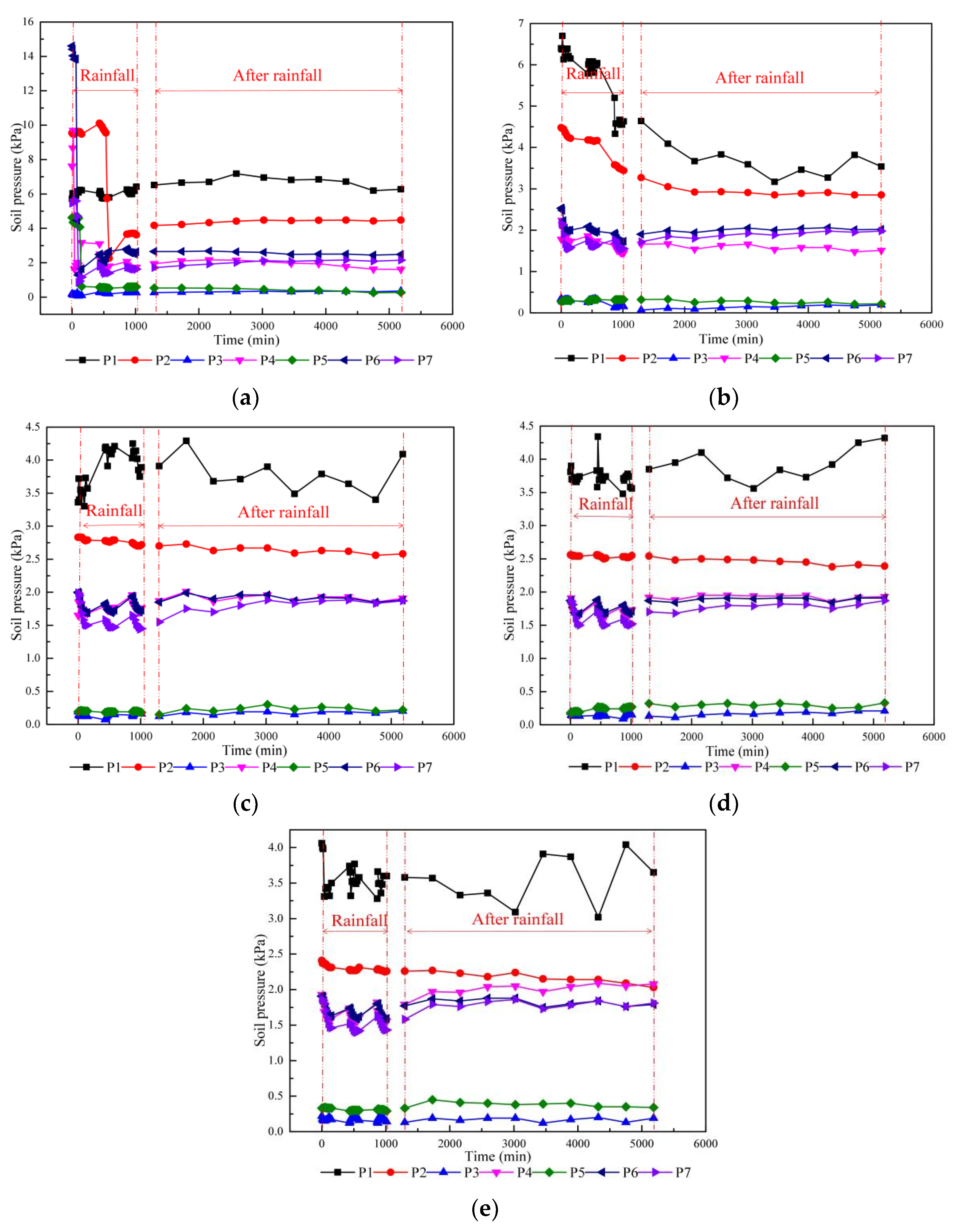
The soil pressure variations of the seven representative points (P1, P2, P3, P4, P5, P6 and P7) over time are shown in Figure 13. During the first round of rainfall, it was in opposition to the developed soil mechanics as the soil pressures of all the representative points except P1 decreased sharply, which was caused by the in situ stress release as the rainwater infiltrated. This was most evident for P6, incorporating a decline from 14.3 kPa to 1.0 kPa in the first round of the rainfall event. After the first round of rainfall, all seven representative points presented no regular variation in the soil pressure with some small fluctuations, representing a relatively steady state of the slope model. Nevertheless, the soil pressure of P1 started to decline in the second round of rainfall, which was later than that of the other points. These results were caused by P1 being in the deepest location, which needed a longer duration for the rainwater influence to occur. Thus, the second deepest point, P2, represented a persistent decrease in soil pressure in the second round, implying that the release of the in situ stress was still in progress in the deeper positions at this duration. In the subsequent rounds, the soil pressure of P2 persistently declined at a smaller rate, as the soil pressure of P1 fluctuated. When the fifth round of rainfall was over, the soil pressures of P1 and P2 were approximately 3.5 kPa and 2.0 kPa, respectively. On the contrary, the soil pressures of the other points were steady over the entire second round, indicating the steady state of the shallower part of the slope model. In summary, induced by the release of in situ stress, the soil pressures in the slope model declined but did not increase, indicating that the influence of the in situ stress release was greater than that of the self-weight increase through rainwater percolation, which is seemingly different from the classical soil mechanics [55]. Classical soil mechanics deems that the saturation of soils increases during rainfall, thus inducing a self-weight increase in the soil. As it does not consider the in situ stress increase inside the soils, theoretically, the soil pressures inevitably increase during the rainfall process. However, in the current study, the slope model construction process exactly simulated the loess-forming process, thus leading to high in situ stress in the slope soils, which was higher than the gravity stress. When the rainwater penetrated, the soils of the slope model were softened and dilated, causing the in situ stress to be released abruptly. As the greatest portion of the in situ stress is released, the measured soil stress must decrease rather than increase.

4.4. Displacements of the Key Points

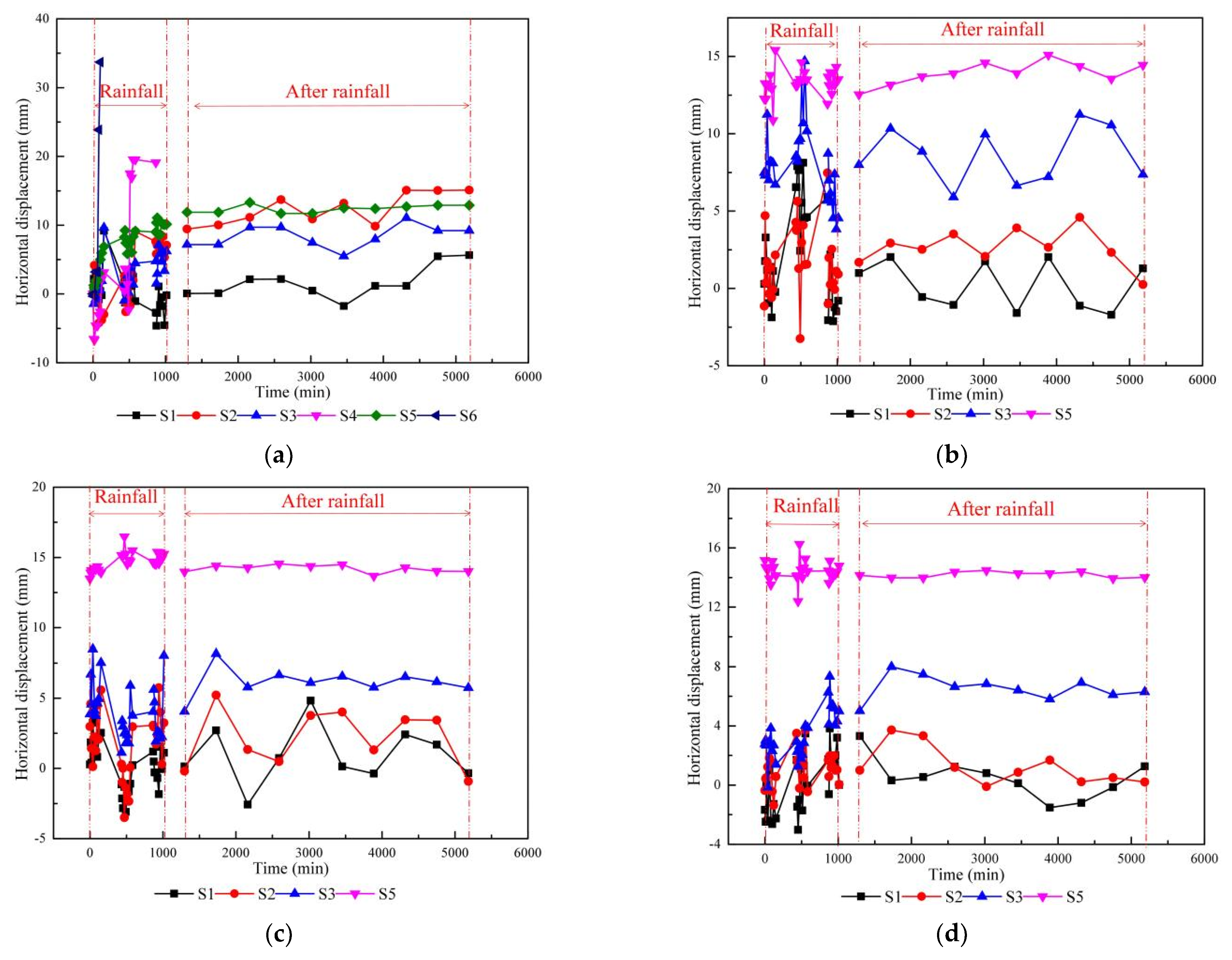
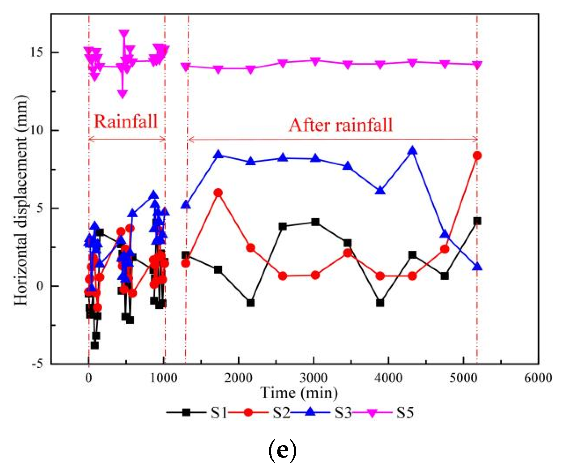
A laser rangefinder was used to measure the distances between the six key points (S1, S2, S3, S4, S5 and S6) and a fixed point, the changes in which before and during the rainfall events were the horizontal displacements of the corresponding positions. Figure 14 presents the variations of the horizontal displacements of the six points over time. In the first round, all six points except S1 had displacements rising from 0 mm, especially within the rainfall events. As the rainfall process advanced, the slope soils were humidified, and the internal frictional angle and the cohesion were lessened, causing the yielding of parts of the model slope, which in turn induced the displacements of the model slope. When the first round of rainfall was over, the horizontal displacements of S2, S3 and S5 rose up to 15.1 mm, 9.2 mm and 12.9 mm, respectively, while that of S1 fluctuated at approximately 0 mm. Understandably, the fluctuations in the displacements were brought about by the errors of the instruments. Additionally, the displacement of S6 rose to approximately 35 mm within the first round of the first rainfall event, and the displacement of S4 rose to approximately 20 mm within the same round of the second rainfall event. According to the rainwater scour data presented earlier, the displacement markers S4 and S6 were destroyed in the first round of the second and first rainfall events, respectively, hence bringing about oddly high increments of displacements. As a result, the figures of displacements do not include those of S4 and S6 after the second round of rainfall.

Within the second round, the displacement for S5 fluctuated up to approximately 14 mm and was still fluctuating around this value in the subsequent rounds. The displacements for S2 and S3 fluctuated at approximately 2.5 mm and 9.2 mm, respectively, as the displacement for S1 kept fluctuating at approximately 0 mm. Reasonably, it could be concluded that point S1 remained stationary during all five rainfall rounds. Considering the points in a vertical line with S1, the longer the upward distance from S1, the larger the displacement. This result indicated that a potential slip surface was situated between S1 and S2. This finding is consistent with the research presented by Cui et al. [56], expressing the landslide progress in five stages: steady deformation, slow deformation, intense deformation, steady deformation and intense deformation. However, it was also found that the displacements of the four remaining points (S1, S2, S3 and S5) fluctuated with no increase after the second round, implying the status of the slope was ultimately stable.

5. Post Evaluation of the Treatment Project

Post evaluation was used in a slope treatment project in China by Zheng [4], who proposed the definition of the post evaluation of slope treatment. During slope design, engineers were concerned about the stability of the slope after the completion of construction. However, in post evaluation, engineers usually focused on the slope stability in the long-term. Zheng proposed a displacement rate threshold of 0.1 mm/day that could be used to judge slope stability. Additionally, a compound safety factor referring to the safety factor of slopes was employed to assess the treatment effect of slopes, presented in

Table 4. Post evaluation criteria of the treatment effect.

Compound Safety Factor (K)	Deformation and Failure Degree (D) %	Displacement Rate (R) mm/d	Treatment Effect
K > 1.20	0.1 < D ≤ 0.5	0.01 < R ≤ 0.05	Very good
1.10 < K ≤ 1.20	0.5 < D ≤ 1.0	0.05 < R ≤ 0.1	Good
1.0 < K ≤ 1.10	1.0 < D ≤ 10	0.1 < R ≤ 0.5	Not bad
K ≤ 1.0	R ≤ 0.1 or D > 10	R ≤ 0.01 or R > 0.5	Conservative or failed

. Considering the deformation and failure extent, some quantitative standards [4] were also adopted into the post evaluation of the slope treatment effect, as shown in Table 4. In accordance with the employed standards, this section continues the post evaluation of the slope prototype using the field investigation and model test data.

5.1. Post Evaluation Based on the Deformation and Failure Degree

As can be seen in Figure 14, when the fifth round was over, the maximum horizontal displacement of the slope model was approximately 14 mm, delivering the maximum horizontal displacement of the slope prototype of 140 mm. Additionally, the main gully in the first grade of the slope model was approximately 30 cm wide when the fifth round was over, and the entire range of the third grade of the slope model had slid. Accordingly, the ratio of the maximum displacement to the height of the slope was approximately 0.08, and the ratio of the collapsed area to the slope surface area was approximately 0.3. As a result, the collapse ratio could be 30.0%, with an overall collapse having a big influences on the project operation. Additionally, this matched the discoveries from the field investigation (see Figure 2). Hence, the treatment effect of the slope was preliminarily assessed as failed, referring to Zheng’s qualitative criteria.

5.2. Post Evaluation Based on the Displacement Rate

Referring to Figure 14, the maximum displacement was approximately 14 mm of S5 when the fifth round was over, rendering the maximum displacement of the prototype as 140 mm at the end of the five years. Therefore, the average deformation rate of the slope project during the 5 years was approximately 0.08 mm/day, implying the security of the treatment project. Thus, the treatment project of the current slope was preliminarily evaluated as good, referring to the qualitative criteria of Zheng.

5.3. Post Evaluation Based on the Compound Safety Factor

The Morgenstern–Price method is a widely accepted way of calculating the safety factors of earth slopes, with a function to generate the slide surface considering every interslice force and satisfying every equilibria of the forces [57,58]. This section utilized the Morgenstern–Price method within the Geo Studio software to delineate the potential slide surface, with well-matched discoveries, as shown in Figure 14. The soil pressures from the model test were utilized to calculate the sliding force and resistance to sliding, thus delivering the factor of safety for the slope prototype. Incorporating Table 4, the treatment effect of the current slope was assessed.

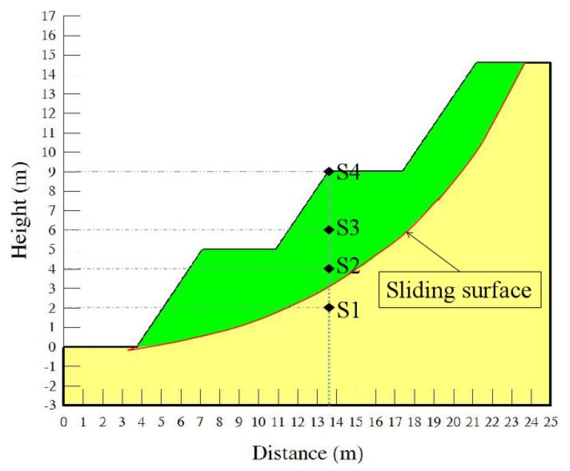
Figure 15 illustrates the potential sliding surface by the end of the fifth year from the Morgenstern–Price method. Evidently, the generated sliding surface was situated between S1 and S2, which strictly matched the model test results.

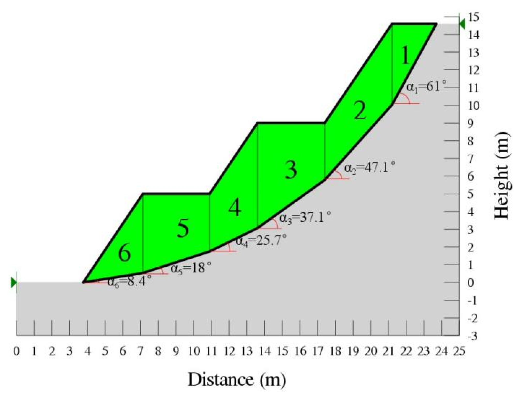
Firstly, the sliding body was divided into six vertical slices, as shown in Figure 16. The measured data of the key points were utilized to derive the soil pressures and suction of the adjacent slices. In this way, the soil pressure and suction values on the bottoms of the slices were obtained, as shown in

Table 5. Sliding slice information.

Slice Number	1	2	3	4	5	6
σy (kPa)	19.45	9.46	6.63	5.68	12.30	19.90
us (kPa)	96.45	52.66	37.60	32.58	67.72	85.42
B (m)	2.6	3.8	3.7	2.8	3.7	3.5
αi (°)	61	47.1	37.1	25.7	18	8.4
Fresisting (kN)	219.01	166.92	121.12	78.29	143.77	160.67
Fsliding (kN)	43.9959	26.24204	14.7186	6.83872	14.1081	10.4475

.

Referring to Equation (7), the safety factor of the slope was:

$$\begin{array}{ll}K& =\frac{{\displaystyle \sum F_{resisting}}}{{\displaystyle \sum F_{sliding}}}\\ & =\frac{889.79 (kN)}{116.35 (kN)}\\ & =7.65\end{array}$$

(12)

Clearly, the safety factor from the developed method combined with the model test data was substantially larger than the critical value of 1.2, implying the conservative design theory of the slope treatment research. This result was likely caused by the underestimation of the shear strength of loess in the slope treatment design theory of China, which did not incorporate the matrix suction under unsaturated conditions. Nevertheless, the obtained safety factor here delivers a result identical to those of the displacements from the model test. Combined with Table 4, it can be seen that the preliminary treatment effect of the slope prototype was very good.

5.4. Post Evaluation of Results

Combining the above post evaluation results, it can be considered that the slope prototype was generally stable, with no further sliding tendency, but considerably large amounts of destruction resulting from rainwater scouring. Accordingly, the destruction of the slope was categorized as a local collapse. Therefore, the treatment effect of the current slope was determined to be not bad.

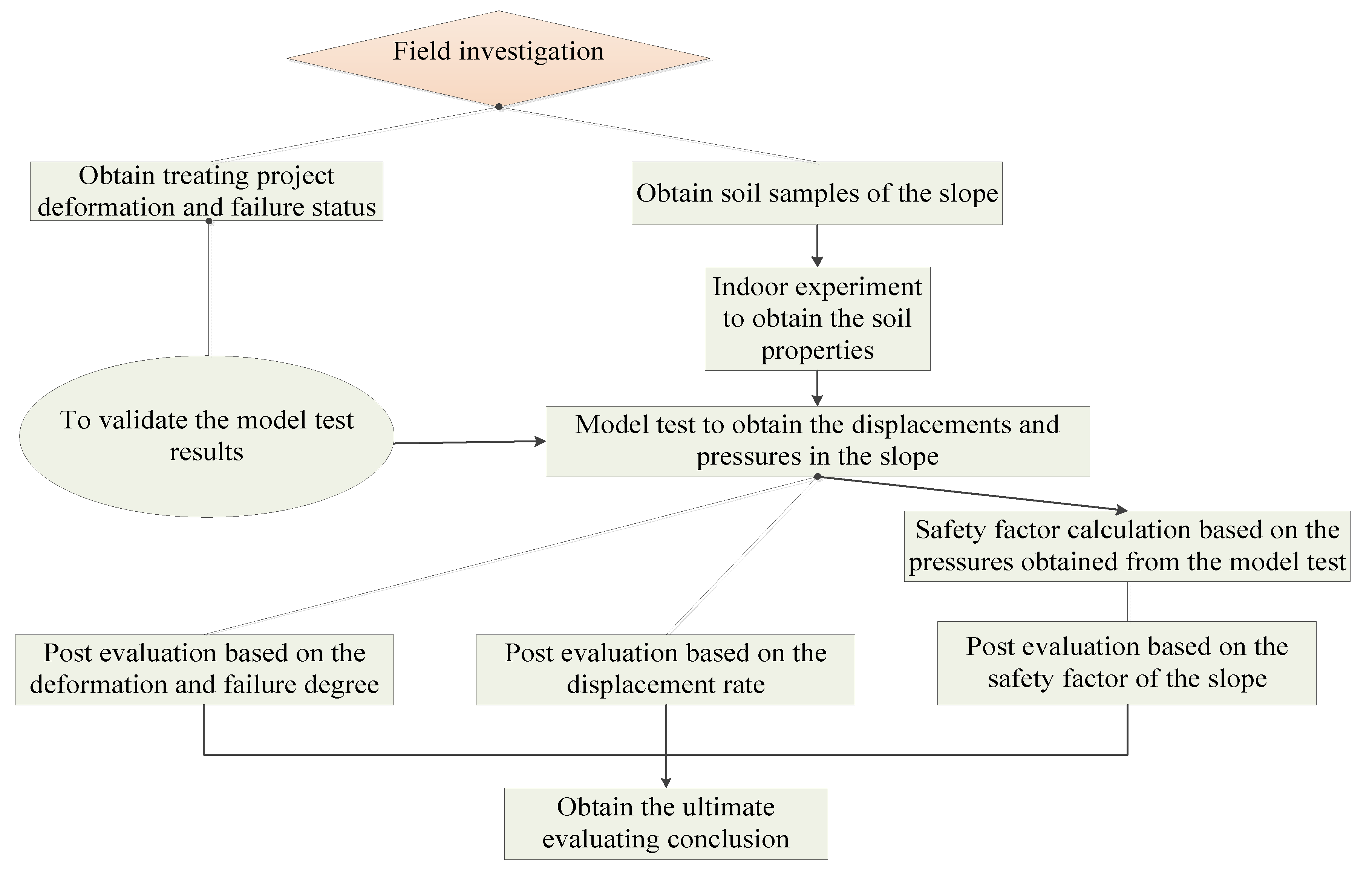
Last, it is worth noting that the post evaluation framework formed here is useful to other slope treatment projects referring to slope cutting. Therefore, the post evaluation framework is presented in Figure 17.

6. Conclusions

To clarify the influencing mechanism of long-term rainfall on loess slopes treated by slope cutting in Yan’an city of Shaanxi Province, a field investigation and an indoor model test were performed, based on the post evaluation of the loess slope with slope cutting. The main conclusions are as follows:

(1)

The runoff of rainwater has serious scouring effects on slope surfaces, causing gullies and shallow slides. Mainly caused by the consolidation of the shallow soils within intervals of rainfall, the scouring effect becomes increasingly weaker over time, inducing a relatively steady state of the slope after the first round of rainfall.

(2)

Rainwater percolates the platforms preferentially with large rates being observed where rainwater pools. Over the simulation duration, the wetting front advancement rate declined gradually.

(3)

Caused by the release of in situ stress, the test soil pressures within the model slope declined drastically during the first rainfall round, especially for the deep positions inside the slope model.

(4)

The horizontal displacements of the critical positions within the slope model increased evidently during the first round, with declining rates. After the second rainfall round, the horizontal displacements showed no regular rise, indicating the ultimately stable status of the slope.

(5)

The model test results were utilized to perform the post evaluation of the slope-cutting treatment to the loess slope, forming a framework for the post evaluations of loess slopes under long-term rainfall. This evaluation framework can be of benefit to other slope treatment projects.