What Causes Haze Pollution? An Empirical Study of PM_2.5 Concentrations in Chinese Cities

Abstract

In recent years, many areas of China have suffered from serious haze pollution, which greatly affects human health and daily life. It is of policy importance to understand the factors that influence the spatial concentration of PM_2.5. Based on data from 74 cities with PM_2.5 monitoring stations in 2013 and 2014, this study presents the overall haze situation in China and explores the determinants of PM_2.5 using a random-effects model, as well as a set of OLS regressions. The results indicate that PM_2.5 is significantly correlated with the industrial proportion, the number of motor vehicles, and household gas consumption, while public financial expenditure on energy saving and environmental protection does not show statistically significant effects. The analysis implies that China should adjust its economic structure and optimizes environmental governance to effectively respond to haze pollution.

1. Introduction

In recent years, serious hazy weather has befallen many areas of China, from the north through the center, and to the Pearl River Delta [1,2,3,4]. Among the pollutants contributing to hazy weather, particulate matter (PM) has attracted much attention [5,6]. PM can be categorized according to its diameter into PM_2.5–10 (coarse PM, with a diameter between 2.5 μm and 10 μm), PM_2.5 (fine PM, with a diameter less than 2.5 μm), and PM₁₀, the sum of the first two [7]. All of these PM threaten human health, although PM_2.5 poses the greatest risk. Based on air pollution data for metropolitan areas throughout the United States, Pope et al. [8] found that a 10 μg per cubic meter increase in the PM_2.5 concentration would increase the all-cause mortality, cardiopulmonary mortality, and lung cancer mortality rates by 4%, 6%, and 8%, respectively. Franklin et al. [9] calculated that a 10 μg per cubic meter increase in the PM_2.5 concentration would increase respiratory-related and stroke-related mortality rates by 1.78% and 1.03%, respectively. These figures are more than triple those recently reported for PM₁₀.

Effective control of PM_2.5 concentrations in China is an urgent priority following recent haze events [6,10]. In 2012, the newly-revised Environment and Air Quality Standard was issued jointly by the Ministry of Environmental Protection of China (MOEP) and China’s General Administration of Quality Supervision, Inspection, and Quarantine (CGAQSIQ) [11]. The standard clarified the first-class ambient air quality functional area and the second-class ambient quality functional area, the former of which contains natural reserve areas, scenic spots, and other areas needing special protection, while the latter contains residential zones, residence-commerce-transportation mixed districts, cultural areas, industrial zones, and rural areas. According to the standard, the annual average concentration of PM_2.5 in the first-class ambient air quality functional area should be limited to 15 μg per cubic meter, and the daily concentration should be limited to 35 μg per cubic meter; the annual average concentration of PM_2.5 in the second-class ambient air quality functional area should be limited to 35 μg per cubic meter, and the daily measure should be limited to 75 μg per cubic meter. In September 2013, the Air Pollution Control Action Plan was issued by the State Council, which clearly proposed that from 2012, PM₁₀ concentrations should decrease by 10% in prefecture-level cities and above, and PM_2.5 concentrations in the Beijing-Tianjin-Hebei region, Yangtze River Delta and Pearl River Delta should decrease by 25%, 20% and 15%, respectively, within which the annual PM_2.5 concentration in Beijing should be controlled at around 60 μg per cubic meter by 2017 [12]. Given the policy importance of the haze pollution issue, it is imperative to understand why some regions have more severe PM_2.5 concentrations than others.

Current research on the determinants of PM_2.5 can be divided into two main streams. The first stream of literature focuses on exploring the source and formation of PM_2.5 by decomposing PM_2.5 from the physical and chemical perspectives [13,14,15,16]. For example, Huegin et al. found a decreasing trend in the concentration of PM_2.5 trace elements, such as Ba, Ca, Ce, Cu, Fe, La, Mo, Mn, Pb, Sb, and Rh from urban streets to urban surroundings, and to rural areas, indicating that road traffic may be the main source of these elements [17]. Based on the main chemical species, some scholars have used the positive matrix factorization (PMF) method to analyze the source of PM_2.5 from eight sources: biomass burning (11%), secondary sulfates (17%), secondary nitrates (14%), coal combustion (19%), industry (6%), motor vehicles (6%), road dust (9%), and yellow dust [18]. Zhang et al. compared the contributions of emissions and weather conditions to regional haze and discovered that primary aerosol was closely related to emission intensity, while the formation and variation in the overall concentration of secondary aerosol were determined by weather conditions in a region [19].

The second stream of literature explores the factors affecting PM_2.5 using statistical methods to analyze monitoring data in sporadic regions. Eeftens et al. [20] explored the effects of transportation intensity, land use, and population density on the spatial variation of PM_2.5 using land use regression. Based on the data for indoor PM_2.5 concentrations in six European cities, Lai et al. explored the effects of smoking, gas-stove usage, outdoor temperature, traffic, heating, cooking, ventilation, and urban or suburban location, and found that indoor PM_2.5 concentrations were greatly affected by smoking, gas-stove usage, outdoor temperature, and wind speed [21]. Wu et al. conducted a series of field studies and found that commuters’ levels of exposure to PM_2.5 were affected by their commuting modes. Specifically, the on-road way mode (walking, bicycle, and motorcycle) showed a higher PM_2.5 concentration (76 μg/m³) than the in-cabin mode (bus, taxi, and metro). Meanwhile, exposure to PM_2.5 under different commuting modes was affected by temperature, humidity, wind direction, and speed [22].

The literature also presents a number of areas that warrant further examination. Current research mainly focuses on the formation of PM_2.5 from the physical and chemical perspectives, but a comprehensive exploration of its antecedents from a macro perspective based on a nationwide sample is needed. Furthermore, although some studies on PM_2.5 concentrations focus on social and natural factors, they do not examine the effects of economic structure and environmental pollution governance. Using the concentration of PM_2.5 (the main component of haze) as the dependent variable, this study explored the factors influencing patterns of PM_2.5 concentration based on statistical data from 74 cities nationwide in 2013 and 2014, focusing on the effects of economic structure and environmental expenditure while controlling for social and natural factors.

2. Overall Status of Haze Pollution in China

After the newly-revised Environment and Air Quality Standard was issued, the Ministry of Environmental Protection of China (MOEP) also published its monitoring and implementation plan at the first stage [23]. The plan requires establishing monitoring stations in some cities located in the priority areas (Beijing-Tianjin-Hebei region, Yangtze River Delta, and Pearl River Delta), in four municipalities governed by the central government directly (Beijing, Shanghai, Tianjin, and Chongqing), in provincial capitals, and in the five cities with independent planning authority (Dalian, Qingdao, Ningbo, Xiamen, and Shenzhen) first. According to this plan, the total number of cities with PM_2.5 monitoring stations would amount to 74 in 2013. 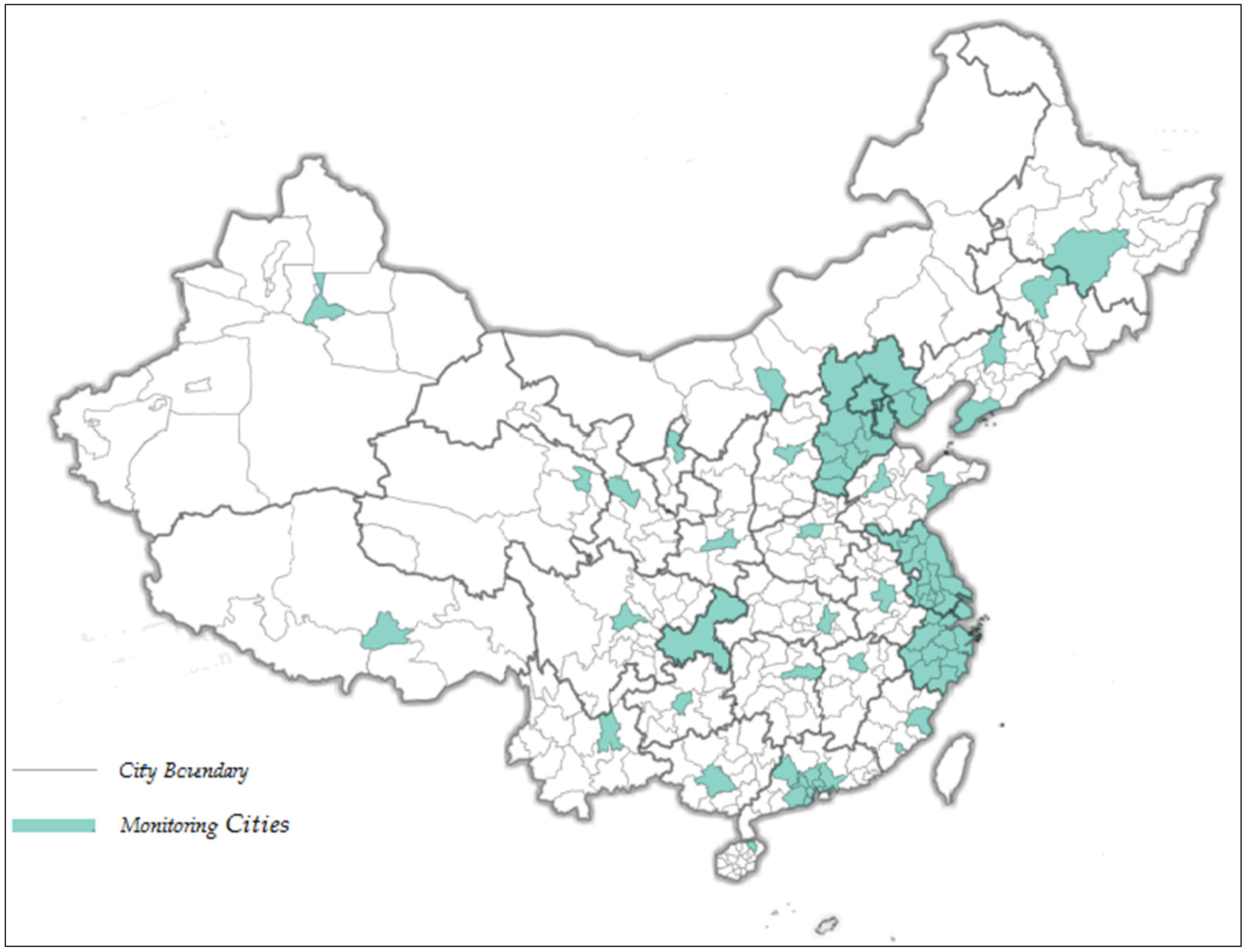The newly installed PM_2.5 monitoring equipment needs to meet the criteria of the Requirement and Technical Indicators of PM_2.5 Automatic Monitoring Equipment issued by the China National Environmental Monitoring Centre [24] and the number of monitoring stations in each city varies from four to 12. All of these 74 cities would have to finish establishing monitoring equipment before October 2012 and begin to publish monitoring data by December 2012. The geographical distribution of these cities with established PM_2.5 monitoring stations by 2013 are shown in Figure 1. Next, we will present the overall status of haze pollution of these 74 cities from a comparative perspective.

Figure 1. The geographical distribution of 74 monitoring cities in China.

Figure 1. The geographical distribution of 74 monitoring cities in China.

2.1. PM_2.5 in Chinese Cities from 2013 to 2014

In February 2012, the newly-amended Environment and Air Quality Standard was issued, which added new monitoring indicators for PM_2.5 and ozone. It specified that the annual average concentration of PM_2.5 in second-class ambient air quality functional areas was to be limited to 35 μg per cubic meter. At the beginning of 2013, 74 cities in China adopted the new standard, set up PM_2.5 monitoring stations and began to release PM_2.5 concentration data, including four direct-controlled municipalities, the capital cities of 27 provinces (except Hong Kong and Macao), and some other prefecture-level cities. Hence, the data are highly representative of different areas across China. In January 2014 and 2015, based on the daily average PM_2.5 concentrations issued by these PM_2.5 monitoring stations and calculated by the arithmetic average method, Greenpeace (in Chinese “Lv Se He Ping”) ranked the annual average PM_2.5 concentrations of the 74 cities above in 2013 and 2014 and published them on the Internet (Table 1). In 2013, the mean of the annual average PM_2.5 concentration in these 74 cities was 70.16 μg per cubic meter, which is twice as high as the new standard of PM_2.5 for second-class ambient air quality functional areas; only five of the 74 cities (6.8%), Fuzhou, Zhoushan, Xiamen, Haikou, and Lhasa, met the standard of 35 μg per cubic meter for the annual average PM_2.5 concentration in second-class ambient air quality functional areas. In 2014, the mean of the annual average PM_2.5 concentration in these 74 cities declined to 62.38 μg per cubic meter, which is still 0.782 times higher than the new standard of PM_2.5 for second-class ambient air quality functional areas; additionally, the number of cities meeting the standard of 35 μg per cubic meter for the annual average PM_2.5 concentration in second-class ambient air quality functional areas also increased to nine, from five.

Table 1. PM_2.5 concentrations in 74 monitoring cities: 2013–2014.

Year = 2013; Average = 70.16						Year = 2014; Average = 62.38
R	City	PM	R	City	PM	R	City	PM	R	City	PM
1	Xingtai	155.2	38	Suzhou	67.1	1	Xingtai	131.4	38	Shaoxing	60.7
2	Shijiazhuang	148.5	39	Yancheng	67	2	Baoding	127.2	39	Lianyungang	60.4
3	Baoding	127.9	40	Jiaxing	66.9	3	Shijiazhuang	122.6	40	Nantong	60.3
4	Handan	127.8	41	Quzhou	66.5	4	Handan	114.2	41	Qinhuangdao	59
5	Hengshui	120.6	42	Shaoxing	66.4	5	Hengshui	107.6	42	Lanzhou	58.8
6	Tangshan	114.2	43	Hangzhou	66.1	6	Langfang	99.3	43	Yancheng	57.5
7	Jinan	114	44	Qinhuangdao	65.2	7	Tangshan	98.4	44	Jiaxing	56
8	Langfang	113.8	45	Chongqing	63.9	8	Jinan	91	45	Qingdao	53.9
9	Xi’an	104.2	46	Xining	63.2	9	Cangzhou	88	46	Chengde	53.5
10	Zhengzhou	102.4	47	Qingdao	61.7	10	Zhengzhou	87.6	47	Quzhou	53.2
11	Tianjin	95.6	48	Shanghai	60.7	11	Tianjin	85.8	48	Zhaoqing	53.1
12	Cangzhou	93.6	49	Hohhot	59.1	12	Beijing	83.2	49	Dalian	53
13	Beijing	90.1	50	Wenzhou	56.5	13	Hefei	80	50	Shanghai	52.2
14	Wuhan	88.7	51	Zhaoqing	54.7	14	Wuhan	79.5	51	Nanchang	49.8
15	Chengdu	86.3	52	Nanning	54.7	15	Xi’an	75.7	52	Nanning	47.6
16	Urumqi	85.2	53	Taizhou	53	16	Changsha	75	53	Guangzhou	47.4
17	Hefei	84.9	54	Foshan	52.3	17	Nanjing	73.7	54	Yinchuan	47.4
18	Taizhou	80.9	55	Guangzhou	52.2	18	Chengdu	72.8	55	Taizhou	46.3
19	Huai’an	80.8	56	Chengde	51.5	19	Harbin	72.5	56	Ningbo	45.7
20	Changsha	79.1	57	Dalian	50.7	20	Taizhou	71	57	Wenzhou	45.7
21	Wuxi	75.8	58	Ningbo	50.4	21	Shenyang	70.9	58	Guiyang	45.5
22	Harbin	75.7	59	Guiyang	49.4	22	Taiyuan	67.7	59	Dongguan	44.1
23	Changzhou	75.6	60	Jiangmen	48.4	23	Suqian	67.6	60	Foshan	44
24	Nanjing	75.3	61	Lishui	47.9	24	Xuzhou	66.7	61	Hohhot	44
25	Xuzhou	74.9	62	Zhongshan	47.6	25	Huai’an	66.5	62	Lishui	43.7
26	Taiyuan	74.2	63	Dongguan	46	26	Wuxi	66.3	63	Jiangmen	43.1
27	Huzhou	73.5	64	Yinchuan	43.7	27	Changzhou	66.2	64	Zhongshan	37.6
28	Shenyang	72.7	65	Zhangjiakou	43.1	28	Zhenjiang	65.8	65	Xiamen	36.3
29	Zhenjiang	71.6	66	Shenzhen	39.7	29	Changchun	64.6	66	Huizhou	34.6
30	Yangzhou	71.1	67	Zhuhai	37.9	30	Jinhua	64.2	67	Zhangjiakou	34.3
31	Suqian	70.7	68	Huizhou	37.2	31	Suzhou	64.1	68	Zhuhai	33.8
32	Nantong	70.2	69	Kunming	35.5	32	Yangzhou	63.2	69	Shenzhen	32.5
33	Changchun	69.2	70	Fuzhou	33.2	33	Urumqi	62.9	70	Kunming	32.2
34	Nanchang	69.1	71	Zhoushan	32.1	34	Huzhou	62.8	71	Fuzhou	31.4
35	Jinhua	69	72	Xiamen	31.3	35	Chongqing	62.8	72	Zhoushan	29.8
36	Lianyungang	68	73	Lhasa	26	36	Xining	62.1	73	Lhasa	23.6
37	Lanzhou	67.1	74	Haikou	25.6	37	Hangzhou	60.9	74	Haikou	22.4

Note: R means the ranking of one city’s PM_2.5 concentration, PM indicates the PM_2.5 concentration, Spearman’s correlation = 0.969, p = 0.000; the unit of PM_2.5 is μg per cubic meter.

Table 1. PM_2.5 concentrations in 74 monitoring cities: 2013–2014.

Year = 2013; Average = 70.16						Year = 2014; Average = 62.38
R	City	PM	R	City	PM	R	City	PM	R	City	PM
1	Xingtai	155.2	38	Suzhou	67.1	1	Xingtai	131.4	38	Shaoxing	60.7
2	Shijiazhuang	148.5	39	Yancheng	67	2	Baoding	127.2	39	Lianyungang	60.4
3	Baoding	127.9	40	Jiaxing	66.9	3	Shijiazhuang	122.6	40	Nantong	60.3
4	Handan	127.8	41	Quzhou	66.5	4	Handan	114.2	41	Qinhuangdao	59
5	Hengshui	120.6	42	Shaoxing	66.4	5	Hengshui	107.6	42	Lanzhou	58.8
6	Tangshan	114.2	43	Hangzhou	66.1	6	Langfang	99.3	43	Yancheng	57.5
7	Jinan	114	44	Qinhuangdao	65.2	7	Tangshan	98.4	44	Jiaxing	56
8	Langfang	113.8	45	Chongqing	63.9	8	Jinan	91	45	Qingdao	53.9
9	Xi’an	104.2	46	Xining	63.2	9	Cangzhou	88	46	Chengde	53.5
10	Zhengzhou	102.4	47	Qingdao	61.7	10	Zhengzhou	87.6	47	Quzhou	53.2
11	Tianjin	95.6	48	Shanghai	60.7	11	Tianjin	85.8	48	Zhaoqing	53.1
12	Cangzhou	93.6	49	Hohhot	59.1	12	Beijing	83.2	49	Dalian	53
13	Beijing	90.1	50	Wenzhou	56.5	13	Hefei	80	50	Shanghai	52.2
14	Wuhan	88.7	51	Zhaoqing	54.7	14	Wuhan	79.5	51	Nanchang	49.8
15	Chengdu	86.3	52	Nanning	54.7	15	Xi’an	75.7	52	Nanning	47.6
16	Urumqi	85.2	53	Taizhou	53	16	Changsha	75	53	Guangzhou	47.4
17	Hefei	84.9	54	Foshan	52.3	17	Nanjing	73.7	54	Yinchuan	47.4
18	Taizhou	80.9	55	Guangzhou	52.2	18	Chengdu	72.8	55	Taizhou	46.3
19	Huai’an	80.8	56	Chengde	51.5	19	Harbin	72.5	56	Ningbo	45.7
20	Changsha	79.1	57	Dalian	50.7	20	Taizhou	71	57	Wenzhou	45.7
21	Wuxi	75.8	58	Ningbo	50.4	21	Shenyang	70.9	58	Guiyang	45.5
22	Harbin	75.7	59	Guiyang	49.4	22	Taiyuan	67.7	59	Dongguan	44.1
23	Changzhou	75.6	60	Jiangmen	48.4	23	Suqian	67.6	60	Foshan	44
24	Nanjing	75.3	61	Lishui	47.9	24	Xuzhou	66.7	61	Hohhot	44
25	Xuzhou	74.9	62	Zhongshan	47.6	25	Huai’an	66.5	62	Lishui	43.7
26	Taiyuan	74.2	63	Dongguan	46	26	Wuxi	66.3	63	Jiangmen	43.1
27	Huzhou	73.5	64	Yinchuan	43.7	27	Changzhou	66.2	64	Zhongshan	37.6
28	Shenyang	72.7	65	Zhangjiakou	43.1	28	Zhenjiang	65.8	65	Xiamen	36.3
29	Zhenjiang	71.6	66	Shenzhen	39.7	29	Changchun	64.6	66	Huizhou	34.6
30	Yangzhou	71.1	67	Zhuhai	37.9	30	Jinhua	64.2	67	Zhangjiakou	34.3
31	Suqian	70.7	68	Huizhou	37.2	31	Suzhou	64.1	68	Zhuhai	33.8
32	Nantong	70.2	69	Kunming	35.5	32	Yangzhou	63.2	69	Shenzhen	32.5
33	Changchun	69.2	70	Fuzhou	33.2	33	Urumqi	62.9	70	Kunming	32.2
34	Nanchang	69.1	71	Zhoushan	32.1	34	Huzhou	62.8	71	Fuzhou	31.4
35	Jinhua	69	72	Xiamen	31.3	35	Chongqing	62.8	72	Zhoushan	29.8
36	Lianyungang	68	73	Lhasa	26	36	Xining	62.1	73	Lhasa	23.6
37	Lanzhou	67.1	74	Haikou	25.6	37	Hangzhou	60.9	74	Haikou	22.4

Note: R means the ranking of one city’s PM_2.5 concentration, PM indicates the PM_2.5 concentration, Spearman’s correlation = 0.969, p = 0.000; the unit of PM_2.5 is μg per cubic meter.

According to the Greenpeace rankings in 2013, the top 10 cities with the highest PM_2.5 concentrations were Xingtai, Shijiazhuang, Baoding, Hengshui, Tangshan, Jinan, Langfang, Xi’an, and Zhengzhou, while the 10 cities with the lowest PM_2.5 concentrations were Haikou, Lhasa, Xiamen, Zhoushan, Fuzhou, Kunming, Huizhou, Zhuhai, Shenzhen, and Zhangjiakou. These rankings indicate that PM_2.5 pollution is more severe in northern cities than in southern cities. In 2014, the ranking of these cities in PM_2.5 concentrations had changed to some extent and we tested the correlation between these two rankings with the method of Spearman’s correlation analysis. It shows that the correlation coefficient is 0.969, which is significant at the level of 99% (p < 0.01). The results mean that the distribution of haze pollution across cities remained relatively consistent in these two years.

2.2. PM_2.5 Concentrations in Eastern, Central, and Western China

Generally, China can be divided into three major regions, and they are Eastern, Central and Western China, from east to west. Eleven provinces are located in Eastern China (Beijing, Fujian, Guangdong, Hainan, Hebei, Jiangsu, Liaoning, Shandong, Shanghai, Tianjin, and Zhejiang), twelve in Western China (Chongqing, Gansu, Guangxi, Guizhou, Inner Mongolia, Ningxia, Qinghai, Shaanxi, Sichuan, Tibet, Xinjiang, and Yunnan), and eight in Central China (Anhui, Heilongjiang, Henan, Hubei, Hunan, Jiangxi, Jilin, and Shanxi), respectively. Based on mean annual average PM_2.5 concentration data from 74 cities in 2013 and 2014, we present the overall situation of PM_2.5 pollution (including the mean, maximum, and minimum values of PM_2.5 concentration and the standard deviations) in the Eastern, Central, and Western China, respectively (see Table 2). The mean in the 54 eastern cities was 1.02 and 0.801 times higher than the new standard in 2013 and 2014 respectively; the mean in the eight central cities was about 2.3 and 2.06 times as high as the new standard in 2013 and 2014, respectively; and the mean in the 12 western cities was 0.76 and 0.513 times higher than the new standard in 2013 and 2014, respectively. In all areas, the mean of the annual average PM_2.5 concentration has exceeded the new standard in both 2013 and 2014. Overall, the mean of the annual average PM_2.5 concentration in the central region was the highest, followed by the eastern and western regions. Meanwhile, the standard deviation of the annual average PM_2.5 concentration in the central region was the lowest, indicating little variation of the haze pollution in this area. However, the city with the most serious haze pollution is located in Eastern China, according to the maximum annual average PM_2.5 concentration in 2013 and 2014.

Table 2. PM_2.5 concentrations in sample Eastern, Central, and Western China cities.

Regions	Sample	Year = 2013				Year = 2014
		Mean	Min	Max	S.D.	Mean	Min	Max	S.D.
East	54	70.56	25.6	155.2	29.2	63.04	22.4	131.4	25.34
Central	8	80.41	69.1	102.4	11.27	72.09	49.8	87.6	11.58
West	12	61.53	26	104.2	22.34	52.95	23.6	75.7	15.7

Note: the unit of PM_2.5 is μg per cubic meter.

Table 2. PM_2.5 concentrations in sample Eastern, Central, and Western China cities.

Regions	Sample	Year = 2013				Year = 2014
		Mean	Min	Max	S.D.	Mean	Min	Max	S.D.
East	54	70.56	25.6	155.2	29.2	63.04	22.4	131.4	25.34
Central	8	80.41	69.1	102.4	11.27	72.09	49.8	87.6	11.58
West	12	61.53	26	104.2	22.34	52.95	23.6	75.7	15.7

Note: the unit of PM_2.5 is μg per cubic meter.

We used analysis of variance (ANOVA) to examine the differences in PM_2.5 concentrations between Eastern, Central, and Western China (ANOVA) (see Table 3). The difference between the mean PM_2.5 concentrations in cities in Eastern China and those in Central China was −9.8514 and −9.0486 μg per cubic meter in 2013 and 2014, respectively; the difference between mean PM_2.5 concentrations in cities in Eastern China and those in Western China was 9.0361 and 10.0889 μg per cubic meter in 2013 and 2014, respectively; the difference between mean PM_2.5 concentrations in cities in Central China and those in Western China was 18.8875 and 19.1375 μg per cubic meter in 2013 and 2014, respectively. None of these differences was statistically significant in 2013 or 2014 (p > 0.05). This means that there is no significant difference between these three regions in a statistical sense, while PM_2.5 pollution in the central region was the most severe.

Table 3. Variance analysis of PM_2.5 concentrations in sample cities.

Regions	Year = 2013			Year = 2014
	Mean Difference	S.D.	p Value	Mean Difference	S.D.	p Value
East-Central	−9.8514	10.2094	0.338	−9.0486	8.72643	0.303
East-West	9.0361	8.6006	0.297	10.0889	7.35135	0.174
Central-West	18.8875	12.3006	0.129	19.1375	10.51385	0.073

Note: the unit of PM_2.5 is μg per cubic meter.

Table 3. Variance analysis of PM_2.5 concentrations in sample cities.

Regions	Year = 2013			Year = 2014
	Mean Difference	S.D.	p Value	Mean Difference	S.D.	p Value
East-Central	−9.8514	10.2094	0.338	−9.0486	8.72643	0.303
East-West	9.0361	8.6006	0.297	10.0889	7.35135	0.174
Central-West	18.8875	12.3006	0.129	19.1375	10.51385	0.073

Note: the unit of PM_2.5 is μg per cubic meter.

2.3. PM_2.5 Concentrations in Three Major Industrial Regions

The Beijing-Tianjin-Hebei region, Yangtze River Delta, and Pearl River Delta are the top three industrial zones in China. Among the 74 cities with PM_2.5 monitoring stations, 13 cities are located in the Beijing-Tianjin-Hebei region, 25 cities in the Yangtze River Delta, and nine cities in the Pearl River Delta. We present the overall situation of PM_2.5 pollution (including the means, the number of times the mean annual PM_2.5 concentration exceeded the standard, the number of cities that met the new standard, and the proportions) in the three major industrial zones of China in 2013 and 2014 (see Table 4). The mean annual PM_2.5 concentrations in these three major industrial regions all exceeded the new standard in these two years. Hardly any of the cities in the Beijing-Tianjin-Hebei area or the Pearl River Delta, and only one city in the Yangtze River Delta, Zhoushan, met the new standard for PM_2.5 in 2013. Haze pollution in these three major industrial regions was clearly very serious in 2013 and remained severe in 2014 in spite of an improving trend. Nevertheless, the means of the annual PM_2.5 concentrations gradually became lower from the north to the south in terms of the geographic locations of the Beijing-Tianjin-Hebei region, the Yangtze River Delta, and the Pearl River Delta.

Table 4. PM_2.5 concentrations in three major industrial regions.

Region	Sample	Year = 2013			Year = 2014
		Mean	Times Larger Than the Standard	Number and Proportion of Cities Meeting the Standard	Mean	Times Larger Than the Standard	Number and Proportion of Cities Meeting the Standard
Beijing-Tianjin-Hebei	13	104	1.97	0 (0%)	92.65	1.65	1 (7.7%)
Yangtze River Delta	25	67	0.91	1 (4%)	58.82	0.68	1 (4%)
Pearl River Delta	9	47	0.34	0 (0%)	41.13	0.18	3 (33.3%)

Note: the unit of PM_2.5 is μg per cubic meter.

Table 4. PM_2.5 concentrations in three major industrial regions.

Region	Sample	Year = 2013			Year = 2014
		Mean	Times Larger Than the Standard	Number and Proportion of Cities Meeting the Standard	Mean	Times Larger Than the Standard	Number and Proportion of Cities Meeting the Standard
Beijing-Tianjin-Hebei	13	104	1.97	0 (0%)	92.65	1.65	1 (7.7%)
Yangtze River Delta	25	67	0.91	1 (4%)	58.82	0.68	1 (4%)
Pearl River Delta	9	47	0.34	0 (0%)	41.13	0.18	3 (33.3%)

Note: the unit of PM_2.5 is μg per cubic meter.

We also examined the differences in PM_2.5 concentrations in three major industrial regions using ANOVA (Table 5). The difference between the mean PM_2.5 concentrations in the cities in the Beijing-Tianjin-Hebei region and those in the Yangtze River Delta was 37.3031 and 33.8338 μg per cubic meter in 2013 and 2014, respectively (significant at p < 0.01); the difference between cities in the Beijing-Tianjin-Hebei region and those in the Pearl River Delta was 57.4009 and 51.5205 μg per cubic meter in 2013 and 2014, respectively (significant at p < 0.01); and the difference between cities in the Yangtze River Delta and those in the Pearl River Delta was 20.0978 and 17.6867 μg per cubic meter in 2013 and 2014, respectively (significant at p < 0.05). These results indicate that the Beijing-Tianjin-Hebei region suffered the most serious PM_2.5 pollution and the Pearl River Delta suffered the least.

Table 5. Variance analysis of PM_2.5 concentrations in three major industrial regions.

Region	2013			2014
	Mean Difference	S.D.	p-Value	Mean Difference	S.D.	p-Value
Beijing-Tianjin-Hebei–Yangtze River Delta	37.3031	7.3861	0.000	33.8338	5.98068	0.000
Beijing-Tianjin-Hebei–Pearl River Delta	57.4009	9.3666	0.000	51.5205	7.58436	0.000
Yangtze River Delta–Pearl River Delta	20.0978	8.3968	0.019	17.6867	6.79906	0.013

Note: the unit of PM_2.5 is μg per cubic meter.

Table 5. Variance analysis of PM_2.5 concentrations in three major industrial regions.

Region	2013			2014
	Mean Difference	S.D.	p-Value	Mean Difference	S.D.	p-Value
Beijing-Tianjin-Hebei–Yangtze River Delta	37.3031	7.3861	0.000	33.8338	5.98068	0.000
Beijing-Tianjin-Hebei–Pearl River Delta	57.4009	9.3666	0.000	51.5205	7.58436	0.000
Yangtze River Delta–Pearl River Delta	20.0978	8.3968	0.019	17.6867	6.79906	0.013

Note: the unit of PM_2.5 is μg per cubic meter.

3. Methodology

3.1. Empirical Model

$$\begin{array}{l}P{M}_{2.5}\left(i,t\right)={\mathsf{\beta }}_1\times Industr{y}_{i,t-1}+{\mathsf{\beta }}_2\times Housin{g}_{i,t-1}+{\mathsf{\beta }}_3\times Vehicl{e}_{i,t-1}+{\mathsf{\beta }}_4\times H\_consumptio{n}_{i,t-1}+\\ {\mathsf{\beta }}_5\times Expenditur{e}_{i,t-1}+{\mathsf{\beta }}_5\times Contro{l}_{i,t-1}+{\mathsf{\beta }}_6\times Year+\mathsf{\epsilon }\end{array}$$

(1)

The model used in this research is shown in Equation (1). The dependent variable is the city-level mean annual PM_2.5 concentration for the 74 cities in mainland China that monitored PM_2.5 and released air quality information in 2013 and 2014. In this model, i and t represents the city code and year code, respectively. The independent variables are the industrial proportion (Industry_i,t-1), housing construction area (Housing_i,t-1), number of motor vehicles (Vehicle_i,t-1), household gas consumption (H_consumption_i,t-1), and expenditure on energy conservation and environmental protection (Expenditure_i,t-1). Control_i,t-1 is a vector of control variables, while Year and ε represent the year dummy and error term, respectively. In order to mitigate the reverse causality problem, the dependent variable is the PM_2.5 monitoring data for 2013 and 2014, while the independent variables reflect the economic, social, and environmental governance data for the 74 cities in 2012 and 2013, correspondingly.

3.2. Measurement, Data Sources, and Description

According to the air quality monitoring results from the Ministry of Environmental Protection, the primary pollutant in China’s haze pollution is PM_2.5. Therefore, we used the annual average PM_2.5 concentration as the indicator of haze severity. The data were collected from two Greenpeace reports ranking the annual average PM_2.5 concentrations of the 74 cities in 2013 and 2014. Greenpeace collected daily monitoring data for these cities from the official environmental information disclosure platform maintained by the Ministry of Environmental Protection. With the arithmetic average method, they calculated the annual average PM_2.5 concentration in each city, respectively. We also collected about 20 cities’ yearly PM_2.5 concentrations published officially and compared these data with those of Greenpeace, we find that the yearly PM_2.5 concentrations reported by Greenpeace is mostly reliable (Pearson correlation = 0.987, p < 0.01).

The economic development mode of “high growth, high pollution” [10] is one of the most important human factors affecting haze. Therefore, the industrial proportion was selected to measure the economic structure, calculated with the industrial product divided by GDP. The data were collected from the China City Statistical Yearbook (2013 and 2014).

The housing construction area can be used as a measure of construction dust in a region. These data were obtained from the Statistical Yearbook (2013 and 2014) for each province. Motor vehicle ownership can be used to measure the exhaust emission volume in a region. These data were collected from the Statistical Yearbook and the National Economy and Social Development Statistical Bulletin (2013 and 2014). Household gas consumption can be used to measure the emission for household heating. These data were collected from the China City Statistical Yearbook (2013 and 2014). To reflect emission intensity rather than emission size, the municipal district area was divided by the housing construction area, motor vehicle ownership and household gas consumption data.

The government’s investment in environmental governance, measured as expenditure on energy conservation and environmental protection, may significantly improve environmental quality. The proportion of expenditure on energy conservation and environmental protection on GDP was used to measure the effect of public environmental governance, using data from the Report of Financial Budget Execution for each city in 2012 and 2013, as well as from the Statistical Yearbook (2013 and 2014) for each province.

Additionally, we controlled a set of time-varying variables in this work. First, we controlled the economic scale by using the logarithm of GDP and green coverage rate, which were collected from the Statistical Yearbook (2013 and 2014) for each province and the China City Statistical Yearbook (2013 and 2014), respectively. Second, natural factors also have a particular influence on haze. Given the availability of data, rainfall, temperature, and relative humidity were used as control variables for natural factors. The data were collected from the Statistical Yearbook for each city, the National Economy and Social Development Statistical Bulletin and the China Statistical Yearbook for 2013 and 2014. Third, time trend effects were controlled by setting a year dummy variable. Descriptive statistics for all variables are presented in Table 6, including variables’ mean values, maximum values, minimum values, and standard deviations. In light of the panel data structure, it reports the overall, between, and within statistics, respectively.

Table 6. Descriptive statistics.

Variable	Overall (N = 148)				Between (n = 74)			Within (T = 2)
	Mean	Max	Min	S.D.	Max	Min	S.D.	Max	Min	S.D.
PM2.5	66.271	155.2	22.4	25.43	143.3	24	24.999	80.521	52.021	5.0996
Industry (%)	47.113	66.23	22.05	9.411	65.52	22.25	9.3867	51.708	42.518	1.0275
Construction	0.0557	0.4026	0.0023	0.0667	0.3802	0.0026	0.0657	0.1348	−0.0235	0.0130
Vehicle	0.0927	0.6588	0.0057	0.1359	0.6588	0.0062	0.1336	0.2429	−0.0575	0.0272
H_consumption	15.171	1197	0.0077	98.25	598.7	0.08	69.289	613.9	−583.56	69.892
Expenditure	0.0032	0.0219	0.0001	0.0034	0.0173	0.0001	0.0032	0.0096	−0.0032	0.0013
Log(GDP)	11.521	12.335	10.415	0.3629	12.32	10.45	0.3632	11.65	11.393	0.026
Green (%)	40.871	64.45	27.18	4.9453	58.225	28.83	4.7863	47.096	34.646	1.3048
Temperature	15.41	24.6	4.3	4.656	24.45	4.3	4.6549	16.41	14.41	0.398
Rainfall (log)	2.9509	3.3324	2.1188	0.2467	3.3324	2.3195	0.2334	3.5313	2.3706	0.0823
R_humidity	66.824	85	34	10.032	82	36	9.94	71.324	62.324	1.58
Year	0.5	1	0	0.5017	0.5	0.5	0	1	0	0.5017

Table 6. Descriptive statistics.

Variable	Overall (N = 148)				Between (n = 74)			Within (T = 2)
	Mean	Max	Min	S.D.	Max	Min	S.D.	Max	Min	S.D.
PM2.5	66.271	155.2	22.4	25.43	143.3	24	24.999	80.521	52.021	5.0996
Industry (%)	47.113	66.23	22.05	9.411	65.52	22.25	9.3867	51.708	42.518	1.0275
Construction	0.0557	0.4026	0.0023	0.0667	0.3802	0.0026	0.0657	0.1348	−0.0235	0.0130
Vehicle	0.0927	0.6588	0.0057	0.1359	0.6588	0.0062	0.1336	0.2429	−0.0575	0.0272
H_consumption	15.171	1197	0.0077	98.25	598.7	0.08	69.289	613.9	−583.56	69.892
Expenditure	0.0032	0.0219	0.0001	0.0034	0.0173	0.0001	0.0032	0.0096	−0.0032	0.0013
Log(GDP)	11.521	12.335	10.415	0.3629	12.32	10.45	0.3632	11.65	11.393	0.026
Green (%)	40.871	64.45	27.18	4.9453	58.225	28.83	4.7863	47.096	34.646	1.3048
Temperature	15.41	24.6	4.3	4.656	24.45	4.3	4.6549	16.41	14.41	0.398
Rainfall (log)	2.9509	3.3324	2.1188	0.2467	3.3324	2.3195	0.2334	3.5313	2.3706	0.0823
R_humidity	66.824	85	34	10.032	82	36	9.94	71.324	62.324	1.58
Year	0.5	1	0	0.5017	0.5	0.5	0	1	0	0.5017

4. Results and Interpretations

We first developed a panel data set to test our hypotheses, which covers economic, social, governance and natural factors for the 74 cities in 2013 and 2014, with 148 observations. We estimated a random-effects model after a Hausman test which suggests that the difference of the coefficients estimated by the fixed-effects model and the random-effects model is not systematic is accepted, indicating choosing the random-effects model (p = 0.8672). The random-effects model has significant χ² values at the 99% level (p < 0.01) and explains 48.93 percent of overall variance, 48.49 percent of cross-sectional variance, and 63.21 percent of time-varying variance in the dependent variable, respectively (overall R² = 0.4893; between R² = 0.4849; within R² = 0.6321), indicating that it has a good model fit (see model 1 in Table 7). The coefficients of Industry, Vehicle and H_consumption are statistically significant and positive at the 90%, 99%, and 95% levels, respectively. That means the industrial proportion, motor vehicle ownership and household gas consumption prove to have identifiable haze pollution impacts. In line with the expected signs, the coefficient of Construction is positive and the coefficient of Expenditure is negative, but neither of them is significant. This indicates that the hypotheses that the housing construction area, expenditure on energy conservation and environmental protection have positive and negative haze pollution impacts, respectively, are not supported.

In order to test the robustness of the random-effects model, we also ran four ordinary least squares (OLS) regressions based on cross-sectional data in 2013, 2014, and their difference (see models 2–5 in Table 6). Specifically, model 2 is based on data in 2013, model 3 is based on data in 2014, and model 4 improves model 3 by adding one-year lagged PM_2.5 concentrations. To address potential endogeneity problems associated with the inclusion of the lag-term in model 4, we also ran model 5, in which the change of PM_2.5 from 2013 to 2014 is set as the dependent variable and the changes in all explanatory variables from 2013 to 2014 are set as regressors. First, the variance inflation factor (VIF) is calculated for each independent variable and control variable in these four models. All of the values are much lower than the critical value of 10, indicating no serious multicollinearity across these models [25]. All of the regression models have significant F values at the 99% level (p < 0.01), indicating that all of the models fit well. In terms of the R² values, independent variables in model 4 explain the highest percentage of variance in the dependent variable mainly because of the inclusion of one-year lagged PM_2.5 concentrations (96.21% of PM_2.5 variation) as a predictor, while those in model 5 explain the lowest percentage (reaching 19.28% of PM_2.5 variation) because it mainly focuses on changes in PM_2.5 over time under a difference-in-difference estimation. Compared to the between R² in model 1, which focuses on cross-sectional fit in the random-effects model, the R² of model 2 and 3 is quite close to it. However, it seems that the R² of model 5 is much lower than the within R² in model 1, though they both focus on the time variability fit. The main reason may lie in that the difference-in-difference estimation fails to consider how the effects of independent variables’ changes depend on their original values.

Table 7. Regression results for factors affecting PM_2.5.

Variable	Panel Data (Random-Effects)	Cross-Sectional Data (OLS Regression)				Panel Data (Random-Effects)
	Model 1 (Full Samples)	Model 2 (Year = 2013)	Model 3 (Year = 2014)	Model 4 (Year = 2014)	Model 5 (Difference Regression)	Model 6 (Samples in Southern China)
Industry	0.470 * (0.253)	0.522 ** (0.256)	0.549 ** (0.228)	0.171 ** (0.071)	0.263 (0.369)	0.420 ** (0.197)
Construction	23.911 (20.904)	51.156 (30.890)	28.42 (34.25)	−1.918 (8.19)	3.197 (20.9)	5.180 (14.073)
Vehicle	50.989 *** (11.441)	67.23 ** (26.857)	67.923 *** (22.568)	9.424 (6.493)	25.14 ** (12.582)	−16.814 (16.612)
H_consumption	0.005 ** (0.002)	0.216 (0.332)	−0.016 (0.014)	0.003 (0.004)	0.006 * (0.003)	0.509 ** (0.258)
Expenditure	59.617 (184.703)	63.906 (898.161)	−610.486 (568.513)	−45.623 (166.14)	125.11 (233.72)	−299.47 (423.52)
Lag_pm	/	/	/	0.795 *** (0.032)	/	/
Log(GDP)	19.252 *** (6.291)	19.665 *** (6.557)	14.452 ** (5.73)	2.197 (1.561)	35.998 * (21.336)	9.514 * (5.197)
Green	0.03 (0.19)	0.079 (0.548)	0.366 (0.365)	0.126 (0.101)	−0.14 (0.245)	−0.119 (0.181)
Temperature	−1.489 *** (0.05)	0.574 (0.939)	−0.702 (0.734)	−0.424 * (0.219)	−2.439 (1.515)	−3.052 *** (0.709)
Rainfall	−0.965 (5.458)	−38.676 * (20.865)	−18.418 (12.53)	1.919 (3.665)	2.553 (3.794)	0.947 (4.231)
R_humidity	−0.399 * (0.24)	−0.51 (0.408)	−0.53 (0.472)	0.008 (0.13)	−0.425 (0.336)	−0.083 (0.265)
Year	−7.429 *** (0.991)	/	/	/	/	−4.831 *** (0.991)
Within R2	0.6321	/	/	/	/	0.7408
Between R2	0.4849	/	/	/	/	0.5875
Overall R2	0.4893	/	/	/	/	0.5968
R2	/	0.5740	0.5243	0.9621	0.1928	/
Observations	148	74	74	74	74	92
Goodness of fit	χ2 = 244.45 ***	F = 9.93 ***	F = 39.09 ***	F = 364.15 ***	F = 5.16 ***	χ2 = 225.76 ***
Hausman	p = 0.8672	/	/	/	/	p = 0.4637

Note: Robust standard errors are given in parentheses. *** p < 0.01,** p < 0.05,* p < 0.1 (two-tailed).

Table 7. Regression results for factors affecting PM_2.5.

Variable	Panel Data (Random-Effects)	Cross-Sectional Data (OLS Regression)				Panel Data (Random-Effects)
	Model 1 (Full Samples)	Model 2 (Year = 2013)	Model 3 (Year = 2014)	Model 4 (Year = 2014)	Model 5 (Difference Regression)	Model 6 (Samples in Southern China)
Industry	0.470 * (0.253)	0.522 ** (0.256)	0.549 ** (0.228)	0.171 ** (0.071)	0.263 (0.369)	0.420 ** (0.197)
Construction	23.911 (20.904)	51.156 (30.890)	28.42 (34.25)	−1.918 (8.19)	3.197 (20.9)	5.180 (14.073)
Vehicle	50.989 *** (11.441)	67.23 ** (26.857)	67.923 *** (22.568)	9.424 (6.493)	25.14 ** (12.582)	−16.814 (16.612)
H_consumption	0.005 ** (0.002)	0.216 (0.332)	−0.016 (0.014)	0.003 (0.004)	0.006 * (0.003)	0.509 ** (0.258)
Expenditure	59.617 (184.703)	63.906 (898.161)	−610.486 (568.513)	−45.623 (166.14)	125.11 (233.72)	−299.47 (423.52)
Lag_pm	/	/	/	0.795 *** (0.032)	/	/
Log(GDP)	19.252 *** (6.291)	19.665 *** (6.557)	14.452 ** (5.73)	2.197 (1.561)	35.998 * (21.336)	9.514 * (5.197)
Green	0.03 (0.19)	0.079 (0.548)	0.366 (0.365)	0.126 (0.101)	−0.14 (0.245)	−0.119 (0.181)
Temperature	−1.489 *** (0.05)	0.574 (0.939)	−0.702 (0.734)	−0.424 * (0.219)	−2.439 (1.515)	−3.052 *** (0.709)
Rainfall	−0.965 (5.458)	−38.676 * (20.865)	−18.418 (12.53)	1.919 (3.665)	2.553 (3.794)	0.947 (4.231)
R_humidity	−0.399 * (0.24)	−0.51 (0.408)	−0.53 (0.472)	0.008 (0.13)	−0.425 (0.336)	−0.083 (0.265)
Year	−7.429 *** (0.991)	/	/	/	/	−4.831 *** (0.991)
Within R2	0.6321	/	/	/	/	0.7408
Between R2	0.4849	/	/	/	/	0.5875
Overall R2	0.4893	/	/	/	/	0.5968
R2	/	0.5740	0.5243	0.9621	0.1928	/
Observations	148	74	74	74	74	92
Goodness of fit	χ2 = 244.45 ***	F = 9.93 ***	F = 39.09 ***	F = 364.15 ***	F = 5.16 ***	χ2 = 225.76 ***
Hausman	p = 0.8672	/	/	/	/	p = 0.4637

Note: Robust standard errors are given in parentheses. *** p < 0.01,** p < 0.05,* p < 0.1 (two-tailed).

In models 2 and 3, the results show that the industrial proportion and motor vehicle ownership are all positively related to PM_2.5 concentrations, whereas housing construction area, household gas consumption, and expenditure on energy conservation and environmental protection are not. When the variable of one-year lagged PM_2.5 concentrations is plugged into model 4, the industrial proportion still remains statistically significant and positively related to PM_2.5 concentrations, while motor vehicle ownership becomes insignificantly related to PM_2.5 concentrations. This finding indicates that both the industrial proportion and motor vehicle ownership have significant haze pollution impacts, while the effect of the industrial proportion outweighs that of motor vehicle ownership. In line with the result of model 1, effects of the housing construction area and expenditure on energy conservation and environmental protection on haze pollution are not supported. Though household gas consumption is statistically significant and positively related to PM_2.5 in model 1, it becomes insignificant in these three OLS regressions, indicating that the hypothesis that household gas consumption has a haze pollution impact is only partially supported. In model 5, motor vehicle ownership and household gas consumption are positively correlated with PM_2.5, while the industrial proportion becomes insignificant. Taking model 5 being a difference-in-difference estimation into account, the results of model 1–5 imply that industrial development may be a deep-rooted driver of PM_2.5 over the long term, and motor vehicle ownership and household gas consumption just figure as emerging drivers in recent years.

China is a huge country where meteorological conditions are different for each city, which may influence the PM_2.5 concentrations. Though we have controlled for the relative humidity, rainfall, and temperature, some other meteorological variables are missing because of their availability, such as wind and atmospheric pressure. However, China is generally divided into the southern and northern regions, based on the Qinling Mountains-Huaihe River line. The meteorological conditions are different in Southern and Northern China. Hence, in order to take into account meteorological conditions, it is reasonable to do a subsample analysis by splitting cities by Southern and Northern China. Actually, there are 46 cities located in Southern China and 28 cities located in Northern China in the sample for this study. As the sample size in Northern China is too small, we just conducted the subsample analysis with the cities in Southern China (see model 6). The Hausman test also suggests that a random-effects model is accepted (p = 0.4637). Compared to model 1, the coefficients of Industry and H_consumption are still statistically significantly positive (p < 0.05 or p < 0.1), while motor vehicle ownership becomes insignificant. To interpret the results across all six models, it concludes that industrial proportion, motor vehicle ownership, and household gas consumption prove to have identifiable haze pollution impacts, but the most important driver for haze pollution in China is its industrial development, as reflected by industrial proportion.

5. Discussions and Conclusions

Though more and more scholars have begun to pay attention to haze pollution in recent years, our knowledge about it has not kept up in pace with the increased haze pollution. Most previous research mainly explores the components of PM_2.5 and its determinants from a micro perspective, little is known about how China’s economic development strategy is related to PM_2.5 and whether China’s public expenditure on environmental governance is effective to control the pollution of PM_2.5, because few studies have focused on determinants of PM_2.5 from the macro perspective based on nationwide samples. Based on monitoring data from 74 cities with PM_2.5 monitoring stations in 2013 and 2014, this study aims to fill this gap by assessing the overall haze situation in China and exploring the determinants of PM_2.5 using the random-effects model, as well as the OLS regression method. It contributes to the knowledge of the relationships between macro-economic, social, governance factors, and regional PM_2.5 concentrations empirically.

The results show that China suffered from serious haze pollution on the whole, especially in the Beijing-Tianjin-Hebei region. According to the newly amended Environment and Air Quality Standard produced by MOEP and CGAQSIQ in 2012, among the 74 cities that launched PM_2.5 monitoring stations, only five, Haikou, Lhasa, Xiamen, Zhoushan and Fuzhou, met the annual average PM_2.5 concentration standard for the second-class ambient air quality functional area in 2013. Despite a weak improvement trend, haze pollution still remained severe in 2014. In terms of the factors affecting PM_2.5 concentrations, the industrial proportion has the most persistent and identifiable haze pollution impact and may figure as a deep-rooted factor over the long term; motor vehicle ownership and household gas consumption also show weak positive effects on PM_2.5 concentrations and may just figure as emerging drivers in recent years. In addition, the hypothesis that expenditure on energy conservation and environmental protection significantly affect PM_2.5 was not supported, indicating that the expenditure structure of environmental governance needs to be urgently improved in China.

The results reveal some existing problems in Chinese economic and social development and environmental governance. First, the imbalanced economic structure in China’s economy is the underlying reason for hazy weather. According to statistics, the primary, secondary, and tertiary industries in China in 2013 accounted for 10.01%, 43.89% and 46.09% of GDP, compared with around 5%, 30%, and 65%, respectively, in developed countries. The proportion of secondary industry in China is 14% higher than that in an average developed country. The internal structure of secondary industry in China is also imbalanced, with a large proportion of manufacturing and processing industries causing a huge environmental footprint. In addition, regional industries in China share structural convergence. The similarity in industrial structure between Eastern and Central China is 93.5%, while between Central and Western China it is 97.9% [26], indicating that the dominance of secondary industry in GDP is a universal problem facing most regions in China. Moreover, China’s economy follows an extensive development pattern. Energy consumption per unit of GDP in China was 2.5 times higher than the world average in 2013, and China’s carbon intensity in recent years has shown an increasing trend [27], which implies a very high environmental burden under the circumstance of its high economic growth since 1978.

Second, from the perspective of pollutant sources, exhaust emissions from energy consumption and motor vehicles directly contribute to hazy weather. In Chinese energy consumption structure, coal accounts for 68.5% and petroleum for 17.7%. Energy sources such as coal and petroleum generate large quantities of industrial waste gas under such an energy consumption structure. Though China has spent efforts to develop renewable energy, the production of renewable energy is quite limited and China is still faced with many policy challenges in deploying renewable energy, such as lack of policy coordination and consistence, weakness and incompleteness in the incentive system, and an incomplete financing system for renewable energy projects [28]. Another important pollution source is automotive exhaust emissions. One important mechanism of haze formation is the process by which coexistence with NO_x can reduce the environmental capacity for SO₂, leading to rapid conversion of SO₂ to sulfate, because NO₂ and SO₂ have a synergistic effect when they react on the surface of mineral dust [29]. According to data released by the Traffic Management Bureau of the Ministry of Public Security, the number of vehicles nationwide, including automobiles and farm vehicles, exceeded 250 million by the end of 2013, an increase of more than 1 million over the past decade. The threat to the environment from vehicle exhaust emissions has increased due to low emission standards, low-quality automobiles, and skyrocketing car ownership.

Finally, serious problems remain in the public governance of environmental pollution, although governments at all levels have increased investment in air pollution control since the rapid increase in hazy weather. First, it is worthwhile exploring how to improve the efficiency of public financial expenditure for pollution treatment, and the control of pollutant sources should be more targeted at PM_2.5 in the future. Second, under the top-down authoritative system, Chinese government officials at all levels differentiate between pollutants with and without clear stipulations, preferring to control those with clear stipulations first. Therefore, more attention should also be paid to reducing the long-term effects of pollutant emissions, particularly secondary pollutants, rather than focusing only on primary pollutants. Third, haze in China presents a complicated regional picture. The traditional localized and disorganized environmental management mode has reduced the efficiency of haze control, calling for strengthened regional cooperation. Urgent improvements in environmental legislation are also needed, together with better policy implementation and administrative supervision. Finally, China also needs to adopt more powerful market-oriented policy tools to address haze pollutions (e.g., environmental/pollution tax). Nowadays, subsidy is a common policy tool in China and thermal power plants received subsidies of more than 100 billion CNY from the state in 2014. The funds are used to expand reproduction rather than to adopt cleaner production technology. For example, new thermal power production projects increased about 55% in the first half of 2015, which resulted in a sharp expansion of thermal power plants and aggravated haze pollutions [30].

To the best of our knowledge, though this work takes the first step toward addressing the haze pollution from a macro perspective, it still has several limitations that are worth discussing. First, the data were limited to 74 cities with PM_2.5 monitoring stations both in 2013 and 2014. As time goes and more cities are setting up PM_2.5 monitoring stations, data for a larger sample of cities over a longer time series could be used to provide more robust evidence in future. Second, the study aims to explore factors affecting PM_2.5 concentrations based on yearly data. Since all the independent variables are aggregated annual mean values, our measurement cannot reflect the variation across different periods within one year, which may affect the significance of our results. For example, it is easier to suffer from haze pollution in the winter than summer, mainly because the meteorological conditions in the winter favor higher PM_2.5 concentrations. Additionally, the meteorological conditions in different regions of China also exhibit different patterns. Some regions experience relatively stable meteorological conditions but others might experience stronger fluctuations over the year. Hence, more tests of these hypotheses are expected to be conducted using monthly or quarterly panel data set to examine whether there are seasonal differences if possible. Third, because of the availability of data, some factors are missed, such as wind, atmospheric pressure, high buildings, biomass burning, and so on. Terrain conditions can also influence the interregional flow of PM_2.5, but we also fail to control for these factors. Therefore, more proxy variables are needed to measure these factors in further research.