
Optimization and Analysis of a Manufacturing–Remanufacturing–Transport–Warehousing System within a Closed-Loop Supply Chain


Abstract
:1. Introduction
2. Manufacturing–Remanufacturing–Transport–Warehousing Closed-Loop Supply Chain System
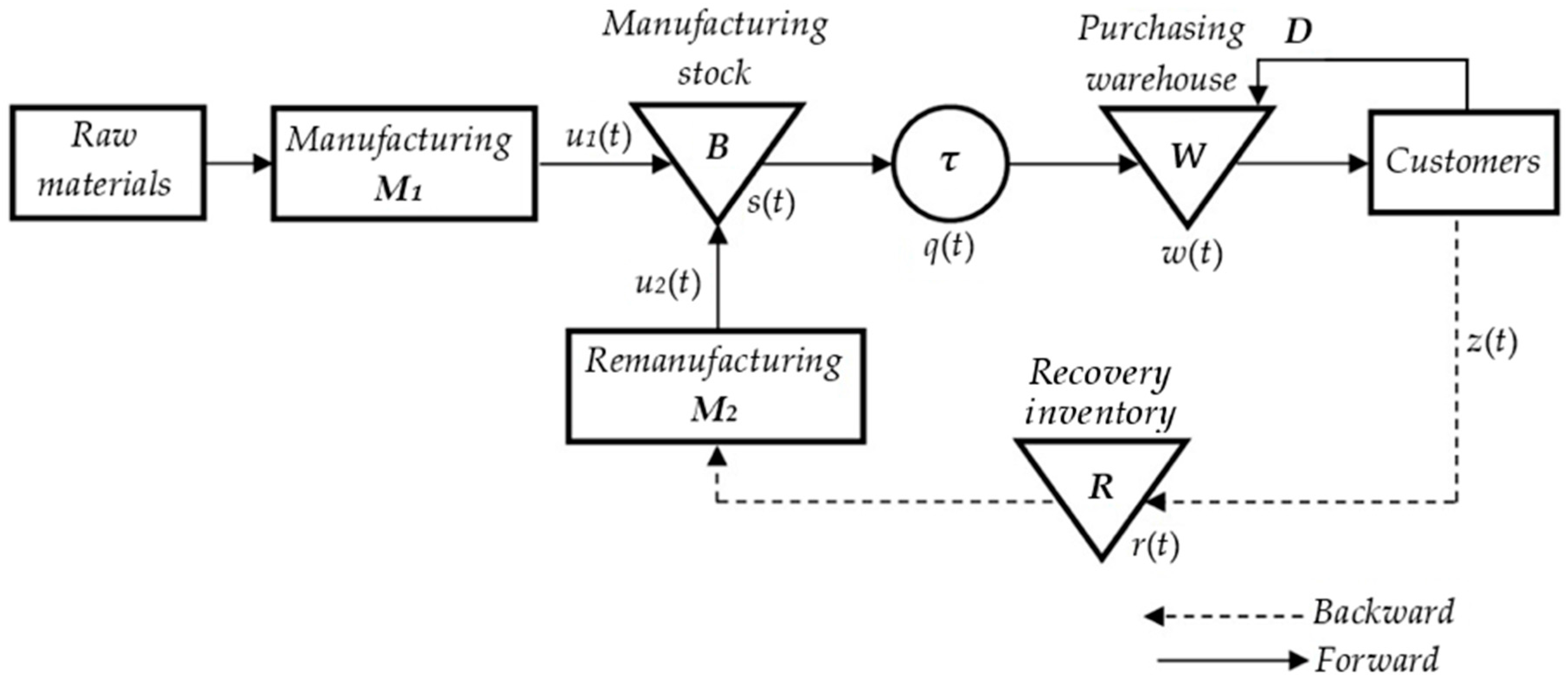
2.1. Notation
| t | instant time. |
| ∆t | time period length. |
| s(t) | manufacturing stock (B) level at time t. |
| S | manufacturing stock capacity. |
| S* | optimal manufacturing stock capacity. |
| g(t) | amount of products outgoing from manufacturing stock S at time t. |
| r(t) | returned products inventory (R) level at time t. |
| D | customers demand at every time t. |
| y(t) | satisfied demand at time t. |
| l(t) | unsatisfied demand at time t. |
| w(t) | purchasing warehouse (W) level at time t. |
| z(t) | returned amount of used end-of-life products at time t. |
| p | percentage relative to the sales of the returned used end-of-life products. |
| p* | optimal percentage relative to the sales of the returned used end-of-life products. |
| q(t) | products being transported at time t. |
| τ | transportation time (the value of transportation time is multiple of Δt). |
| θ | products’ service life. |
| X | purchasing warehouse capacity. |
| X* | optimal purchasing warehouse capacity. |
| V | vehicle capacity. |
| V* | optimal vehicle capacity. |
| α(t) | state of the machine M1 at time t. |
| β(t) | state of the machine M2 at time t. |
| U | maximum production rate of both machines. |
| U1 | maximum production rate of the machine M1. |
| U2 | maximum production rate of the machine M2. |
| u(t) | production rate of M1 and M2 at time t. |
| u1(t) | production rate of the machine M1 at time t. |
| u2(t) | production rate of the machine M2 at time t. |
| MTBF1 | mean time between failures for machine M1. |
| MTBF2 | mean time between failures for machine M2. |
| MTTR1 | mean time to repair for machine M1. |
| MTTR2 | mean time to repair for machine M2. |
| cs | unit inventory holding cost for the manufacturing stock (B). |
| cl | unit lost sales cost. |
| cr | unit inventory holding cost for the returned products (recovery inventory R). |
| ct | unit transportation cost. |
| cw | unit inventory holding cost for purchasing warehouse (W). |
| cu1 | unit manufacturing cost of a product from raw materials. |
| cu2 | unit remanufacturing cost. |
| cz | unit return cost of used products. |
| T | total simulation time. |
| f(t) | cost function at time t. |
| F(T) | total cost function (the objective function). |
2.2. Explanation of the System
- (1)
- In order to simplify the calculations, we assume Δt = 1.
- (2)
- When the demand is not satisfied, loss occurs which results into lost sales costs (l(t)).
- (3)
- To consider transportation time, we assume that τ > 0, known and constant. Indeed, τ is multiple of Δt with τ = m·Δt = m (Δt = 1) and m = {1, 2, 3, …, T}. We assume also that the time for changing and discharging the vehicle is included in the transportation time τ.
- (4)
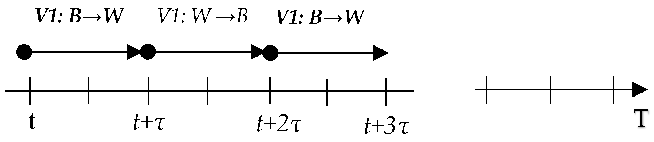
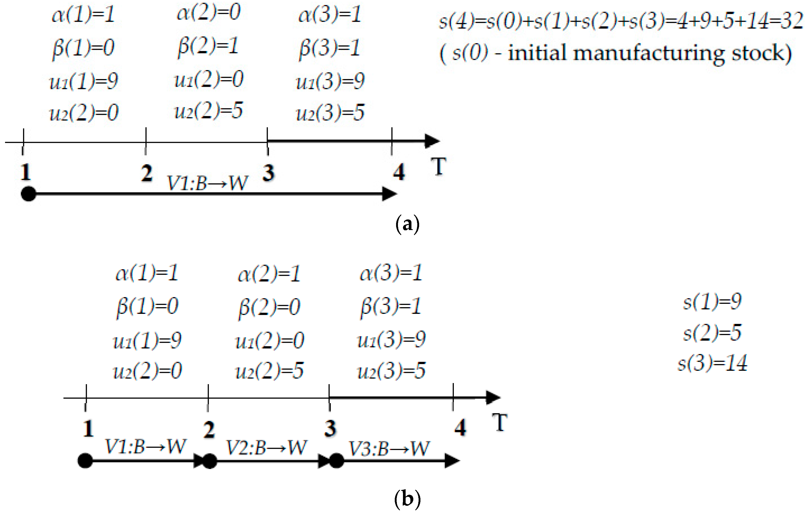
- We assume the case where transport is ensured by two vehicles, vehicle 1 and vehicle 2. When vehicle 1 reaches W, vehicle 2 departs from B and when vehicle 1 comes back to B, vehicle 2 reaches W and vice versa. This assumption allows having one trip from B to W for every τ period and the objective is to reduce the number of trips (see Figure 3: an example when m = 2 we have τ = 2·Δt = 2). This assumption is the usual case of companies that ensure manufacturing and transport of products.
- (5)
- Companies are working to keep a good level service by satisfying customers’ demands. Thus, in inventory management, to avoid having too much lost sales (unsatisfied demand), we must avoid having both manufacturing stock B and purchasing warehouse W is always empty. Thus, we made the following assumptions:
- (5.1)
- Maximum production rate U satisfies the demand (i.e., U ≥ D). This assumption avoids having manufacturing stock B always empty.
- (5.2)
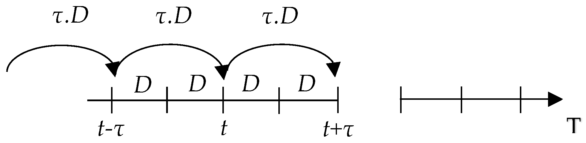
- Purchasing of the warehouse capacity W should be equal or higher than the sum of demands during the transportation time (i.e., X ≥ τ·D). Indeed, the fact that W satisfies the customers demand D at each period and is fulfilled every period equals to the transport time τ = m·Δt. The level of W should be equal or higher than the sum of demands during τ (w(t) ≥ m·D) to satisfy the demands. Thus, if capacity X < τ·D, we always have lost sales. Let us look at the following example (see Figure 4).
If we assume that m = 2 (i.e., τ = 2·Δt = 2) and D = 10 products/period, at the purchasing warehouse, the capacity should be X ≥ τ·D = 2 × 10 = 20.- (5.3)
- The vehicle capacity should also be equal or higher than the sum of the demands during the transportation time (i.e., V ≥ τ·D). Indeed, the vehicle supplies the purchasing warehouse W. If V < τ·D, the level of W will never reach τ·D, and then we always have lost sales.
- (6)
- Maximum production rate U2 is higher than the return amount, (i.e., U2 > z). This assumption avoids having the remanufacturing inventory R always full.
- (7)
- Remanufactured products have the same quality and price as the brand new ones.
- (8)
- We suppose that we have enough parts in the warehouse to satisfy the demand in a given time period t = 0, i.e., w(0) ≥ D.
2.3. Mathematical Model
3. Optimization Based on the Genetic Algorithm
3.1. Interest of Using Optimization Method
3.2. Optimization Method Description
| Algorithm 1 Optimization Algorithm Pseudo-Code |
|
3.3. Conclusion on Optimization Method
4. Numerical Results
4.1. Influence of p on the Optimal Values S*, V*, X*.
- T = 100,000 periods
- MTBF1 = 4 periods
- MTTR1 = 1 period
- MTBF2 = 4 periods
- MTTR2 = 1 period
- D = 10 products/period
- U1 = 9 products/period
- U2 = 5 products/period
- τ = 1 period
- cu1 = 10 monetary units
- cu2 = 4 monetary units
- cw = 2 monetary units
- cs = 2 monetary units
- cr = 1 monetary unit
- cz = 1 monetary unit
- cl = 250 monetary units
- cq = 1 monetary unit
- θ = 30 periods
4.2. Influence of the Value of Transportation Time (τ) on the Optimal Values p*, S*, V*, and X*
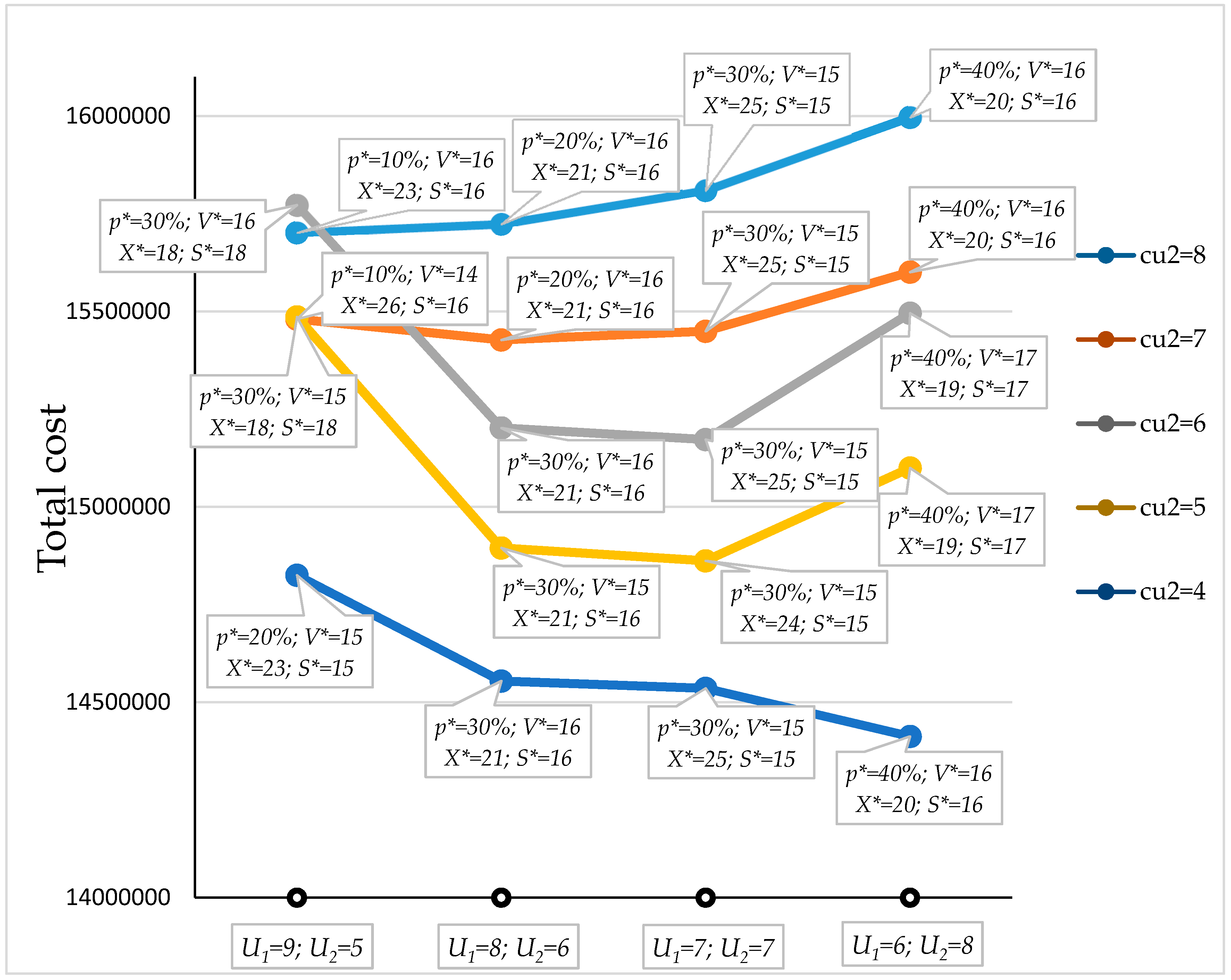
4.3. Influence of Machines Reconfiguration and Unit Manufacturing/Remanufacturing Costs on the Optimal Values p*, S*, V* and X*
- (1)
- U1 = 9 and U2 = 5;
- (2)
- U1 = 8 and U2 = 6;
- (3)
- U1 = 7 and U2 = 7; and
- (4)
- U1 = 6 and U2 = 8.
5. Conclusions
Acknowledgments
Author Contributions
Conflicts of Interest
References
- Galve, J.E.; Elduque, D.; Pina, C.; Javierre, C. Sustainable supply chain management: The influence of disposal scenarios on the environmental impact of a 2400 L waste container. Sustainability 2016, 8, 564. [Google Scholar] [CrossRef]
- Moon, I.; Jeong, Y.J.; Saha, S. Fuzzy Bi-Objective Production-Distribution Planning Problem under the Carbon Emission Constraint. Sustainability 2016, 8, 798. [Google Scholar] [CrossRef]
- Despeisse, M.; Ball, P.D.; Evans, S.; Levers, A. Industrial ecology at factory level—A conceptual model. J. Clean. Prod. 2012, 31, 30–39. [Google Scholar] [CrossRef]
- Liu, C.; Yang, J.; Lian, J.; Li, W.; Evans, S.; Yin, Y. Sustainable performance oriented operational decision-making of single machine systems with deterministic product arrival time. J. Clean. Prod. 2014, 85, 318–330. [Google Scholar] [CrossRef]
- Li, J.; Du, W.; Yang, F.; Hua, G. The carbon subsidy analysis in remanufacturing closed-loop supply chain. Sustainability 2014, 6, 3861–3877. [Google Scholar] [CrossRef]
- Van Nunen, A.E.E.J.; Zuidwijk, R.A. E-enabled closed-loop supply chains. Calif. Manag. Rev. 2004, 46, 40–54. [Google Scholar] [CrossRef]
- Salema, M.I.G.; Povoa, A.P.B.; Novais, A.Q. An Optimization Model for the Design of a Capacitated Multi-Product Reverse Logistics Network with Uncertainty. Eur. J. Oper. Res. 2007, 179, 1063–1077. [Google Scholar] [CrossRef]
- De Brito, M.P.; Dekker, R.; Flapper, S.D.P. Reverse Logistics—A Review of Case Studies; Report Series Research in Management, ERS-2003-012-LIS; Erasmus Research Institute of Management: Berlin, Germany, 2003. [Google Scholar]
- Guide, V.D.R., Jr.; Van Wassenhove, L.N. OR FORUM—The evolution of closed-loop supply chain research. Oper. Res. 2009, 57, 10–18. [Google Scholar] [CrossRef]
- Mitra, S. Inventory management in a two-echelon closed-loop supply chain with correlated demands and returns. Comput. Ind. Eng. 2012, 62, 870–879. [Google Scholar] [CrossRef]
- Kenne, J.P.; Dejax, P.; Gharbi, A. Production planning of a hybrid manufacturing–remanufacturing system under uncertainty within a closed-loop supply chain. Int. J. Prod. Econ. 2012, 135, 81–93. [Google Scholar] [CrossRef]
- Chung, S.L.; Wee, H.M.; Yang, P.C. Optimal Policy for a Closed-Loop Supply Chain Inventory System with Remanufacturing. Math. Comput. Model. 2008, 48, 867–881. [Google Scholar] [CrossRef]
- Turki, S.; Hajej, Z.; Rezg, N. Performance Evaluation of a Hybrid Manufacturing Remanufacturing System Taking Into Account the Machine Degradation. In Proceedings of the 15th IFAC Symposium on Information Control Problems in Manufacturing (INCOM 15), Ottawa, ON, Canada, 11–13 May 2015. [Google Scholar]
- Turki, S.; Rezg, N. Unreliable manufacturing supply chain optimisation based on an infinitesimal perturbation analysis. Int. J. Syst. Sci. Oper. Logist. 2016. [Google Scholar] [CrossRef]
- Turki, S.; Hennequin, S.; Sauer, N. Performances evaluation of a failure-prone manufacturing system with time to delivery and stochastic demand. In Proceedings of the 13th IFAC Symposium on Information Control Problems in Manufacturing (INCOM 09), Moscow, Russia, 3–5 June 2009; Volume 13. [Google Scholar]
- Teunter, R.H. Economic ordering quantities for recoverable item inventory systems. Nav. Res. Logist. 2001, 48, 484–495. [Google Scholar] [CrossRef]
- Tang, O.; Grubbström, R.W. The detailed coordination problem in a two-level assembly system with stochastic lead times. Int. J. Prod. Econ. 2003, 81, 415–429. [Google Scholar] [CrossRef]
- Tang, O.; Grubbström, R.W. Considering stochastic lead times in a manufacturing/remanufacturing system with deterministic demands and returns. Int. J. Prod. Econ. 2005, 93, 285–300. [Google Scholar] [CrossRef]
- Darla, S.P.; Naiju, C.D.; Annamalai, K.; Sravan, Y.U. Production and Remanufacturing of Returned Products in Supply Chain using Modified Genetic Algorithm. World Acad. Sci. Eng. Technol. Int. J. Mech. Aerosp. Ind. Mechatron. Manuf. Eng. 2012, 6, 574–577. [Google Scholar]
- Kelle, P.; Silver, E.A. Purchasing Policy of New Containers Considering the Random Returns of Previously Issued Containers. IIE Trans. 1989, 21, 349–354. [Google Scholar] [CrossRef]
- Toktay, L.B.; Wein, L.M.; Zenios, S.A. Inventory management of remanufacturable products. Manag. Sci. 2000, 46, 1412–1426. [Google Scholar] [CrossRef]
- Sadok, T.; Nidhal, R. Perturbation analysis for discrete flow model: Optimization of a manufacturing-remanufacturing system. In Proceedings of the 2014 IEEE International Conference on Systems, Man and Cybernetics (SMC), San Diego, CA, USA, 5–8 October 2014; pp. 2569–2574. [Google Scholar]
- Yao, C.; Cassandras, C.G. Using infinitesimal perturbation analysis of stochastic flow models to recover performance sensitivity estimates of discrete event systems. Discret. Event Dyn. Syst. 2012, 22, 197–219. [Google Scholar] [CrossRef]
- Xie, X.; Hennequin, S.; Mourani, I. Perturbation analysis and optimisation of continuous flow transfer lines with delay. Int. J. Prod. Econ. 2013, 51, 7250–7269. [Google Scholar] [CrossRef]
- Mourani, I.; Hennequin, S.; Xie, X. Simulation-based optimization of a single-stage failure-prone manufacturing system with transportation delay. Int. J. Prod. Econ. 2008, 112, 26–36. [Google Scholar] [CrossRef]
- Falkenauer, E. A hybrid grouping genetic algorithm for bin packing. J. Heuristics 1996, 2, 5–30. [Google Scholar] [CrossRef]
- Rubinowitz, J.; Levitin, G. Genetic algorithm for assembly line balancing. Int. J. Prod. Econ. 1995, 41, 343–354. [Google Scholar] [CrossRef]
- Akella, R.; Kummar, P.R. Optimal control of production rate in failure prone manufacturing system. IEEE Trans. Autom. Control 1986, 31, 116–126. [Google Scholar] [CrossRef]
- Lia, Y.; Yub, J.; Ta, D. Genetic algorithm for spanning tree construction in P2P distributed interactive applications. Neurocomputing 2014, 140, 185–192. [Google Scholar] [CrossRef]
- Lasheen, M.; Abdel Rahman, A.K.; Abdel-Salam, M.; Ookawara, S. Performance enhancement of constant voltage based MPPT for photovoltaic applications using genetic algorithm. Energy Procedia 2016, 100, 217–222. [Google Scholar] [CrossRef]
- Cornejo-Bueno, L.; Nieto-Borge, J.C.; Garcia-Diaz, P.; Rodriguez, G.; Salcedo-Sanz, S. Significant wave height and energy flux prediction for marine energy applications: A grouping genetic algorithm—Extreme Learning Machine approach. Renew. Energy 2016, 97, 380–389. [Google Scholar] [CrossRef]
- Sauvey, C.; Sauer, N. A genetic algorithm with genes-association recognition for flowshop scheduling problems. J. Intell. Manuf. 2012, 23, 1167–1177. [Google Scholar] [CrossRef]


| p | S* | V* | X* | F(T) |
|---|---|---|---|---|
| 10% | 16 | 15 | 27 | 15,022,529 |
| 20% | 15 | 15 | 23 | 14,824,557 |
| 30% | 15 | 14 | 19 | 15,148,097 |
| 40% | 14 | 13 | 17 | 41,847,037 |
| 50% | 11 | 11 | 11 | 214,821,535 |
| τ | p* | S* | V* | X* | F(T) | τ·d | X*/(τ·d) |
|---|---|---|---|---|---|---|---|
| 1 | 20% | 15 | 15 | 23 | 14,824,557 | 10 | 2.3 |
| 2 | 30% | 29 | 29 | 29 | 18,562,953 | 20 | 1.45 |
| 3 | 30% | 38 | 38 | 38 | 21,981,917 | 30 | 1.27 |
| 4 | 30% | 48 | 48 | 48 | 25,292,159 | 40 | 1.20 |
| 5 | 30% | 58 | 58 | 58 | 28,251,540 | 50 | 1.16 |
| 6 | 30% | 68 | 68 | 68 | 31,413,165 | 60 | 1.13 |
| 7 | 30% | 77 | 77 | 77 | 34,594,556 | 70 | 1.10 |
| 8 | 30% | 86 | 86 | 86 | 37,115,528 | 80 | 1.07 |
| 9 | 30% | 96 | 96 | 96 | 40,614,008 | 90 | 1.06 |
| 10 | 30% | 104 | 104 | 104 | 43,707,006 | 100 | 1.04 |
| cs | cw | τ | P* | S* | V* | X* | F(T) |
|---|---|---|---|---|---|---|---|
| 1 | 4 | 4 | 30% | 66 | 40 | 56 | 27,729,534 |
| 4 | 1 | 4 | 20% | 46 | 46 | 65 | 26,453,331 |
| U1 | U2 | cu1 | cu2 | P* | V* | X* | S* | COST |
|---|---|---|---|---|---|---|---|---|
| 9 | 5 | 10 | 4 | 20% | 15 | 23 | 15 | 14,824,557 |
| 8 | 6 | 10 | 4 | 30% | 16 | 21 | 16 | 14,553,720 |
| 7 | 7 | 10 | 4 | 30% | 15 | 25 | 15 | 14,535,097 |
| 6 | 8 | 10 | 4 | 40% | 16 | 20 | 16 | 14,411,959 |
© 2017 by the authors. Licensee MDPI, Basel, Switzerland. This article is an open access article distributed under the terms and conditions of the Creative Commons Attribution (CC BY) license (http://creativecommons.org/licenses/by/4.0/).
Share and Cite
Turki, S.; Didukh, S.; Sauvey, C.; Rezg, N. Optimization and Analysis of a Manufacturing–Remanufacturing–Transport–Warehousing System within a Closed-Loop Supply Chain. Sustainability 2017, 9, 561. https://doi.org/10.3390/su9040561
Turki S, Didukh S, Sauvey C, Rezg N. Optimization and Analysis of a Manufacturing–Remanufacturing–Transport–Warehousing System within a Closed-Loop Supply Chain. Sustainability. 2017; 9(4):561. https://doi.org/10.3390/su9040561
Chicago/Turabian StyleTurki, Sadok, Stanislav Didukh, Christophe Sauvey, and Nidhal Rezg. 2017. "Optimization and Analysis of a Manufacturing–Remanufacturing–Transport–Warehousing System within a Closed-Loop Supply Chain" Sustainability 9, no. 4: 561. https://doi.org/10.3390/su9040561
APA StyleTurki, S., Didukh, S., Sauvey, C., & Rezg, N. (2017). Optimization and Analysis of a Manufacturing–Remanufacturing–Transport–Warehousing System within a Closed-Loop Supply Chain. Sustainability, 9(4), 561. https://doi.org/10.3390/su9040561