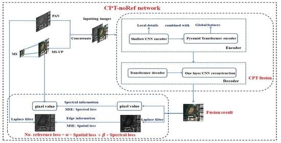
Figure 1.
The fusion framework.
Figure 1.
The fusion framework.
Figure 2.
The preprocessing of training data.
Figure 2.
The preprocessing of training data.
Figure 3.
The architecture of CNN.
Figure 3.
The architecture of CNN.
Figure 4.
The pyramid Transformer encoder.
Figure 4.
The pyramid Transformer encoder.
Figure 5.
Converting to patches.
Figure 5.
Converting to patches.
Figure 6.
The MSA structure.
Figure 6.
The MSA structure.
Figure 7.
Transformer encoder structure.
Figure 7.
Transformer encoder structure.
Figure 8.
The spatial information of (a) fusion, (b) PAN, and (c) MS-UP image.
Figure 8.
The spatial information of (a) fusion, (b) PAN, and (c) MS-UP image.
Figure 9.
, , and QNR indexes of the fusion results with different values of (0.1–0.9): (a) , (b) , and (c) QNR.
Figure 9.
, , and QNR indexes of the fusion results with different values of (0.1–0.9): (a) , (b) , and (c) QNR.
Figure 10.
The visual effect of fusion results with different weight values of (0.1–0.9): (a) 0.1, (b) 0.2, (c) 0.3, (d) 0.4, (e) 0.5, (f) 0.6, (g) 0.7, (h) 0.8, and (i) 0.9.
Figure 10.
The visual effect of fusion results with different weight values of (0.1–0.9): (a) 0.1, (b) 0.2, (c) 0.3, (d) 0.4, (e) 0.5, (f) 0.6, (g) 0.7, (h) 0.8, and (i) 0.9.
Figure 11.
GF-1 true color (R, G, B) fusion results trained by using different loss function: (a) PAN, (b) MS-UP, (c) PNN, (d) TF-ResNet, (e) PanNet, (f) CPT, (g) PNN-noRef, (h) TF-ResNet-noRef, (i) PanNet-noRef, and (j) CPT-noRef (proposed method).
Figure 11.
GF-1 true color (R, G, B) fusion results trained by using different loss function: (a) PAN, (b) MS-UP, (c) PNN, (d) TF-ResNet, (e) PanNet, (f) CPT, (g) PNN-noRef, (h) TF-ResNet-noRef, (i) PanNet-noRef, and (j) CPT-noRef (proposed method).
Figure 12.
WV-2 true color (R, G, B) fusion results trained by using different loss function: (a) PAN, (b) MS-UP, (c) PNN, (d) TF-ResNet, (e) PanNet, (f) CPT, (g) PNN-noRef, (h) TF-ResNet-noRef, (i) PanNet-noRef, and (j) CPT-noRef (proposed method).
Figure 12.
WV-2 true color (R, G, B) fusion results trained by using different loss function: (a) PAN, (b) MS-UP, (c) PNN, (d) TF-ResNet, (e) PanNet, (f) CPT, (g) PNN-noRef, (h) TF-ResNet-noRef, (i) PanNet-noRef, and (j) CPT-noRef (proposed method).
Figure 13.
WV-2 comparison of the details of the objects in PNN trained by different loss functions: The first line is for PNN with reference loss, the second line is for PNN with no-reference loss. (a) the crossroads; (b) the cars; (c) the roof 1; (d) the zebra crossing; and (e) the roof 2.
Figure 13.
WV-2 comparison of the details of the objects in PNN trained by different loss functions: The first line is for PNN with reference loss, the second line is for PNN with no-reference loss. (a) the crossroads; (b) the cars; (c) the roof 1; (d) the zebra crossing; and (e) the roof 2.
Figure 14.
GF-1 true color (R, G, B) fusion results for the urban scenes: (a) PAN, (b) MS-UP, (c) PNN, (d) DRPNN, (e) ResNet, (f) TF-ResNet, (g) GAN, (h) PanNet, (i) improved-SRCNN, and (j) CPT-noRef (proposed method).
Figure 14.
GF-1 true color (R, G, B) fusion results for the urban scenes: (a) PAN, (b) MS-UP, (c) PNN, (d) DRPNN, (e) ResNet, (f) TF-ResNet, (g) GAN, (h) PanNet, (i) improved-SRCNN, and (j) CPT-noRef (proposed method).
Figure 15.
GF-1 false color (NIR, R, G) fusion results for the rural scene 1: (a) PAN, (b) MS-UP, (c) PNN, (d) DRPNN, (e) ResNet, (f) TF-ResNet, (g) GAN, (h) PanNet, (i) improved-SRCNN, and (j) CPT-noRef (proposed method).
Figure 15.
GF-1 false color (NIR, R, G) fusion results for the rural scene 1: (a) PAN, (b) MS-UP, (c) PNN, (d) DRPNN, (e) ResNet, (f) TF-ResNet, (g) GAN, (h) PanNet, (i) improved-SRCNN, and (j) CPT-noRef (proposed method).
Figure 16.
GF-1 true color (R, G, B) fusion results for the rural scene 2: (a) PAN, (b) MS-UP, (c) PNN, (d) DRPNN, (e) ResNet, (f) TF-ResNet, (g) GAN, (h) PanNet, (i) improved-SRCNN, and (j) CPT-noRef (proposed method).
Figure 16.
GF-1 true color (R, G, B) fusion results for the rural scene 2: (a) PAN, (b) MS-UP, (c) PNN, (d) DRPNN, (e) ResNet, (f) TF-ResNet, (g) GAN, (h) PanNet, (i) improved-SRCNN, and (j) CPT-noRef (proposed method).
Figure 17.
WV-2 true color (R, G, B) fusion results in vegetation region: (a) PAN, (b) MS-UP, (c) PNN, (d) DRPNN, (e) ResNet, (f) TF-ResNet, (g) GAN, (h) PanNet, (i) improved-SRCNN, and (j) CPT-noRef (proposed method).
Figure 17.
WV-2 true color (R, G, B) fusion results in vegetation region: (a) PAN, (b) MS-UP, (c) PNN, (d) DRPNN, (e) ResNet, (f) TF-ResNet, (g) GAN, (h) PanNet, (i) improved-SRCNN, and (j) CPT-noRef (proposed method).
Figure 18.
WV-2 true color (R, G, B) fusion results in highway region: (a) PAN, (b) MS-UP, (c) PNN, (d) DRPNN, (e) ResNet, (f) TF-ResNet, (g) GAN, (h) PanNet, (i) improved-SRCNN, and (j) CPT-noRef (proposed method).
Figure 18.
WV-2 true color (R, G, B) fusion results in highway region: (a) PAN, (b) MS-UP, (c) PNN, (d) DRPNN, (e) ResNet, (f) TF-ResNet, (g) GAN, (h) PanNet, (i) improved-SRCNN, and (j) CPT-noRef (proposed method).
Figure 19.
The true color (R, G, B) generalized image testing on Pleiades image: (a) PAN, (b) MS-UP, (c) PNN, (d) DRPNN, (e) ResNet, (f) TF-ResNet, (g) GAN, (h) PanNet, (i) improved-SRCNN, and (j) CPT-noRef (proposed method).
Figure 19.
The true color (R, G, B) generalized image testing on Pleiades image: (a) PAN, (b) MS-UP, (c) PNN, (d) DRPNN, (e) ResNet, (f) TF-ResNet, (g) GAN, (h) PanNet, (i) improved-SRCNN, and (j) CPT-noRef (proposed method).
Figure 20.
The true color (R, G, B) generalized image testing on WV2 image: (a) PAN, (b) MS-UP, (c) PNN, (d) DRPNN, (e) ResNet, (f) TF-ResNet, (g) GAN, (h) PanNet, (i) improved-SRCNN, and (j) CPT-noRef (proposed method).
Figure 20.
The true color (R, G, B) generalized image testing on WV2 image: (a) PAN, (b) MS-UP, (c) PNN, (d) DRPNN, (e) ResNet, (f) TF-ResNet, (g) GAN, (h) PanNet, (i) improved-SRCNN, and (j) CPT-noRef (proposed method).
Table 1.
The information of remote sensing sensor data.
Table 1.
The information of remote sensing sensor data.
| | Band Number | Spatial Resolution/(m) | Location | Landscape |
|---|
| MS | PAN |
|---|
| GF-1 | 1PAN + 4MS | 8 | 2 | Beijing | Rural + Urban |
| Pleiades | 1PAN + 4MS | 2 | 0.5 | Shandong | Urban |
| WV-2 | 1PAN + 8MS | 2 | 0.5 | Washington, DC | Urban |
Table 2.
The parameters of CNN structure.
Table 2.
The parameters of CNN structure.
| 1st ConV | 2st ConV | | 3st ConV |
|---|
| c1 | | f1(x) | c2 | | f2(x) | c3 | | f2(x) | c4 |
| N + 1 | 9 × 9 | ReLU | 16 | 5 × 5 | ReLU | 32 | 5 × 5 | ReLU | 32 |
Table 3.
The basic training parameters settings of the experiment.
Table 3.
The basic training parameters settings of the experiment.
| The Basic Training Parameters |
|---|
| Number of training sets (PAN/MS-UP) | 102,400 |
| Number of test sets (PAN/MS-UP) | 25,600 |
| The size of the training image data | [100 × 100] |
| The size of patch size | 5 |
Table 4.
The hyper-parameters settings of the experiment.
Table 4.
The hyper-parameters settings of the experiment.
| The Hyper-Parameters Settings |
|---|
| The batch size | 16 |
| |
| Number of the hidden nodes in MLP | 2 × F + 1 (F means the number of input features) |
| Number of the heads in MSA | 4 |
Table 5.
GF-1 objective evaluation indexes of the model trained by different loss functions.
Table 5.
GF-1 objective evaluation indexes of the model trained by different loss functions.
| | | | |
|---|
| PNN | 0.8006 | 0.0421 | 0.1642 |
| TF-ResNet | 0.8891 | 0.0727 | 0.0412 |
| PanNet | 0.8530 | 0.1284 | 0.0213 |
| CPT | 0.9201 | 0.0560 | 0.0253 |
| PNN-noRef | 0.9437 | 0.0330 | 0.0241 |
| TF-ResNet-noRef | 0.9531 | 0.0273 | 0.0201 |
| PanNet-noRef | 0.9548 | 0.0314 | 0.0142 |
| CPT-noRef | 0.9675 | 0.0224 | 0.0103 |
Table 6.
WV-2 objective evaluation indexes of the model trained by different loss functions.
Table 6.
WV-2 objective evaluation indexes of the model trained by different loss functions.
| | | | |
|---|
| PNN | 0.7027 | 0.0410 | 0.2673 |
| TF-ResNet | 0.7312 | 0.0237 | 0.2510 |
| PanNet | 0.8380 | 0.0702 | 0.0987 |
| CPT | 0.9015 | 0.0245 | 0.0759 |
| PNN-noRef | 0.8905 | 0.0101 | 0.1004 |
| TF-ResNet-noRef | 0.9086 | 0.0089 | 0.0832 |
| PanNet-noRef | 0.9073 | 0.0214 | 0.0728 |
| CPT-noRef | 0.9283 | 0.0066 | 0.0655 |
Table 7.
GF-1 objective evaluation indexes for the urban scenes.
Table 7.
GF-1 objective evaluation indexes for the urban scenes.
| | | | | | | | |
|---|
| PNN | 0.9648 | 1.0163 | 0.8006 | 0.0421 | 0.1642 | 0.9693 | 1.2815 |
| DRPNN | 0.9720 | 0.9517 | 0.7770 | 0.1310 | 0.1059 | 0.9479 | 1.2076 |
| ResNet | 0.9835 | 0.8389 | 0.8969 | 0.0731 | 0.0324 | 0.9587 | 1.0325 |
| TF-ResNet | 0.9814 | 0.8430 | 0.8891 | 0.0727 | 0.0412 | 0.9593 | 1.1504 |
| GAN | 0.9607 | 1.0829 | 0.6972 | 0.1433 | 0.1862 | 0.9453 | 1.2681 |
| PanNet | 0.9846 | 0.8279 | 0.8530 | 0.1284 | 0.0213 | 0.9486 | 0.9875 |
| Improved-SRCNN | 0.9785 | 0.9498 | 0.8131 | 0.1113 | 0.0851 | 0.9490 | 1.1842 |
| CPT-noRef | 0.9887 | 0.8042 | 0.9675 | 0.0224 | 0.0103 | 0.9876 | 0.8179 |
Table 8.
GF-1 objective evaluation indexes for the rural scenes.
Table 8.
GF-1 objective evaluation indexes for the rural scenes.
| | | | | | | | |
|---|
| PNN | 0.9751 | 0.9320 | 0.8388 | 0.0392 | 0.1270 | 0.9825 | 1.2610 |
| DRPNN | 0.9810 | 0.8420 | 0.8282 | 0.1113 | 0.0681 | 0.9413 | 1.2342 |
| ResNet | 0.9852 | 0.8350 | 0.9073 | 0.0712 | 0.0232 | 0.9601 | 0.9547 |
| TF-ResNet | 0.9824 | 0.8342 | 0.9239 | 0.0521 | 0.0253 | 0.9643 | 0.9530 |
| GAN | 0.9598 | 1.1003 | 0.8002 | 0.0673 | 0.1421 | 0.9619 | 1.3230 |
| PanNet | 0.9873 | 0.8101 | 0.8955 | 0.0925 | 0.0132 | 0.9510 | 0.9421 |
| Improved-SRCNN | 0.9776 | 0.9232 | 0.8240 | 0.1210 | 0.0625 | 0.9421 | 1.0103 |
| CPT-noRef | 0.9895 | 0.7988 | 0.9763 | 0.0136 | 0.0102 | 0.9912 | 0.7213 |
Table 9.
WV-2 objective evaluation indexes.
Table 9.
WV-2 objective evaluation indexes.
| | | | | | | | |
|---|
| PNN | 0.9421 | 1.5258 | 0.7027 | 0.0410 | 0.2673 | 0.9554 | 1.6237 |
| DRPNN | 0.9473 | 1.5227 | 0.7061 | 0.0432 | 0.2620 | 0.9549 | 1.5468 |
| ResNet | 0.9582 | 1.1846 | 0.8088 | 0.0322 | 0.1643 | 0.9643 | 1.3499 |
| TF-ResNet | 0.9495 | 1.3418 | 0.7312 | 0.0237 | 0.2510 | 0.9737 | 1.4429 |
| GAN | 0.9249 | 1.4238 | 0.7058 | 0.0181 | 0.2812 | 0.9797 | 1.7136 |
| PanNet | 0.9731 | 0.8909 | 0.8380 | 0.0702 | 0.0987 | 0.9355 | 0.9631 |
| Improved-SRCNN | 0.9625 | 0.8965 | 0.8433 | 0.0619 | 0.1010 | 0.9445 | 1.1267 |
| CPT-noRef | 0.9873 | 0.8155 | 0.9283 | 0.0066 | 0.0655 | 0.9997 | 0.8313 |
Table 10.
The GF-1 training time (with reference loss on the simulated data).
Table 10.
The GF-1 training time (with reference loss on the simulated data).
| Method/Epoch (Second) | PNN | DRPNN | ResNet | TF-ResNet | GAN | PanNet | Improved-SRCNN | CPT |
|---|
| Average time | 19.576 | 116.350 | 205.124 | 244.562 | 137.058 | 70.940 | 53.194 | 39.809 |
| Epoch number | 150 | 150 | 150 | 250 | 400 | 250 | 250 | 250 |
Table 11.
The GF-1 training time (with a no-reference loss on the real data).
Table 11.
The GF-1 training time (with a no-reference loss on the real data).
| Method/Epoch (Second) | PNN-noRef | TF-ResNet-noRef | PanNet-noRef | CPT-noRef (Proposed) |
|---|
| Average time | 287.543 | 3628.905 | 852.895 | 458.252 |
| Equivalent average time | 17.971 | 226.810 | 53.306 | 28.641 |
| Epoch number | 150 | 250 | 250 | 250 |


