An Integrated Approach for Monitoring Contemporary and Recruitable Large Woody Debris

Abstract

Large woody debris (LWD) plays a critical structural role in riparian ecosystems, but it can be difficult and time-consuming to quantify and survey in the field. We demonstrate an automated method for quantifying LWD using aerial LiDAR and object-based image analysis techniques, as well as a manual method for quantifying LWD using image interpretation derived from LiDAR rasters and aerial four-band imagery. In addition, we employ an established method for estimating the number of individual trees within the riparian forest. These methods are compared to field data showing high accuracies for the LWD method and moderate accuracy for the individual tree method. These methods can be integrated to quantify the contemporary and recruitable LWD in a river system.

1. Introduction

Large woody debris (LWD) plays a critical structural role in riparian ecosystems in forested biomes by providing habitat, guiding channel hydraulics, and mediating stream temperature, amongst other services [1,2,3,4]. In rivers and streams that border areas inhabited by humans, LWD can also pose a risk by damaging infrastructure, such as bridge pilings, creating dangerous hazards for recreational use, and potentially increasing flood risk [5,6,7,8]. The balance of the ecological benefits of LWD and the risks to humans from LWD present a challenge to organizations tasked with managing rivers and streams, creating a need for information on LWD to be used for decision-making.

Field surveys are the traditional method of choice for organizations looking to assess the quantity and spatial location of LWD, but such surveys are very expensive and often lack complete coverage of an area of interest due to limited budgets, time constraints and/or access issues due to property ownership [9]. Remote sensing methodologies provide the potential for detecting LWD, but significant challenges exist due to the small size of LWD and its tendency to be obscured by overstory and understory vegetation. Optical remote sensing using pixel-based analysis techniques have been used to map and identify large accumulations of LWD in areas with little vegetation cover with variable success, typically realizing higher accuracies when pixel sizes are smaller [10,11,12,13]. The lack of vegetation cover reduces problems associated with shadows and occlusion by vegetation. In areas of high vegetation cover, such as forested environments away from riparian area, pixel-based methods have had limited success in mapping LWD [14]. LiDAR-based methods of LWD detection provide an avenue for arriving at information on LWD structure beneath vegetation canopies and without the problem of shadowing. Several studies have either hinted at the potential for LiDAR to detect LWD [15] or used LiDAR to detect a probability of the presence of LWD [16]. Studies that have used LiDAR to directly assess the presence of individual pieces or clumps of LWD have showed some success in forested environments [17,18,19], but these studies examine relatively small areas which limit the interpretation of their accuracy assessments. These studies do highlight that it is possible to filter LiDAR data to produce a raster surface highlighting the presence of LWD.

In this study, we fuse high spatial resolution multi-spectral aerial imagery with discrete-return LiDAR to detect LWD in a complex, forested riparian environment. We use object-based image analysis (OBIA) techniques to produce image objects representing LWD and compare them to field measurements in four different river systems. This portion of the study is referred to as the “LWD Analysis” and its purpose is to establish the accuracy of quantifying contemporary LWD. In addition, we extended the results of the LWD analysis by incorporating a technique to identify and count individual trees (IT) using LiDAR and calibrated with field data. The purpose of this analysis, termed the “IT Analysis” is to establish the accuracy of quantifying recruitable LWD. The results of the two analyses are used to provide an example integrated analysis for monitoring LWD.

2. Materials and Methods

2.1. Study Area

Four river systems were used in this study, all located within King County, WA, USA (Figure 1), Riparian areas in all four systems are partially developed with a mix of single family homes, parking lots, roads, bridges, dikes, and revetments, but all five river ecosystems also contain undeveloped riparian areas consisting of vegetated flood plains and gravel bars. The principle riparian trees are black cottonwood (Populus trichocarpa), big leaf maple (Acer macrophyllum), and red alder (Alnus rubra), with occasional Douglas-fir (Pseudotsuga menzeisii) and Western red-cedar (Thuja plicata). Small multi-stemmed shrubs and brambles are also common. The rivers range in width from 20 to 30 m wide, and all experience seasonal flooding in the rainy season.

Study sites within the river systems were selected to coincide with the 2013 LiDAR coverage (Figure 1) and to include a minimum of five plots of each plot type (individual tree (IT) and large woody debris (LWD)) within each of the five riparian areas: the Cedar River, Green River, Raging River, and Middle and Upper Snoqualmie Rivers. An additional five plots were installed in the Cedar River for a total of 10 of each type. The data from the Cedar River were intended to be used to build the LWD identification ruleset, while the other river systems were intended to be used as validation. A completely randomized study design was infeasible due to the scarcity of LWD and suitable treed areas within each of the riparian zones, so plots were selected manually using orthophotos. Individual tree (IT) plots were 0.04 ha circular plots and were selected so that the plot center was approximately 12 m from the bank location, at least 20 m from any other IT plot center, and contained at least two trees. Plots were also selected so that they would be on public lands and be accessible for the field crew. LWD plots were selected by identifying log jams or areas of wood accumulation visible from the orthophotos, accessible to the field crew, and not on private property. A rectangle was drawn around the LWD plot in ArcGIS to delineate the boundaries. Figure 1 gives the locations of all plots selected in the study.

2.2. Field Data Acquisition

The field crew consisted of two trained individuals who visited each plot location. For IT plots, the field crew used a Trimble GeoXH GPS (Trimble Navigation Ltd., Sunnyvale, CA, USA) unit to navigate to the plot center. A Leica Builder Total Station was set up over the plot center and used to survey individual tree locations and GPS locations. Two GPS locations were collected with the Trimble GeoXH in relatively open canopy locations with a minimum of 100 points that were later differentially corrected with Trimble Pathfinder. The spatial location of each individual tree within the plot boundary and larger than 30.5 cm diameter at breast height (DBH) was recorded with the total station by shooting to the center of the tree. In addition, the species, DBH, height, crown base height, and crown diameter (measured along two perpendicular axes were also measured. Figure 2 and Figure 3 show histograms of the variability in tree DBH and tree height across all field plots. Figure 1C shows an example of an IT plot. Note that in the example of Figure 1, one tree surveyed with the total station was found in post-processing to be out of the plot and, thus, excluded from further analysis.

The location of each LWD plot was found using the Timble GeoXH, and the GPS was then used to mark out the pre-selected plot corners. It was important to make sure that all LWD were completely within the plot, so the crew moved the plot corners or added additional corners to ensure all LWD to be surveyed was within the plot. The spatial location of each corner was recorded with the Total Station and two GPS points were collected and surveyed with the total station using the same methods as the IT plots. Each piece of LWD that was greater than 30 cm in diameter at it largest end was surveyed by collecting points at its two ends. If one end of the LWD was buried in the substrate, the end point was recorded at the point of burial. The diameters of each end were measured with a DBH tape if it was possible to string the tape around the LWD. If this was not possible, a ruler was used to measure the diameter by laying the ruler over the LWD and visually assessing the diameter from a close distance. Figure 1D shows an example of an LWD plot. Individual pieces of LWD that were covered by other LWD and, thus, not visible or accessible to the field crew were not surveyed. The measurement of individual LWD were modeled as rhombi by using the two measured diameters as two of the sides and the measured length as the other two sides. The area of each rhombus was computed to produce a measure of surface area in order for comparison to LWD surface area generated using remotely-sensed data.

2.3. Remotely Sensed Data Acquisition, Processing, and Statistical Analysis

Aerial LiDAR and four-band (blue, green, red, and near-infrared) imagery were acquired in leaf-off conditions in the spring of 2013. The aerial imagery was acquired with an Ultracam Falcon at 0.15 m pixel resolution. The LiDAR data were acquired with a Leica ALS70 with an average pulse density of greater than eight pulses per m² and processed as discrete returns with horizontal and vertical accuracy greater than 0.15 m. For the LWD analysis, the raw LiDAR points (all returns) were used along with the vendor-provided bare Earth model to produce a raster of the elevation above ground level of the highest point within 1.83 m of the ground surface for a raster with a cell size of 0.15 m. This raster filtered out tree canopy and tall shrubs while maintaining the fine detail surface characteristics that a standard vendor supplied digital elevation model smooths. A ruleset was built in eCognition 8.0 (Trimble Navigation Ltd., Sunnyvale, CA, USA) using data only for the Cedar River by importing the processed LiDAR elevation raster and the four band imagery. The initial step of the ruleset found all image objects greater than 0.2 m in elevation. Subsequent steps in the ruleset filtered non LWD objects based on area, asymmetry, rectangular fit, ratio of length to width, and NDVI (the normalized difference vegetation index, calculated as the ratio of the difference in digital numbers of the near infrared and red bands to the sum of the near-infrared and red bands). The ruleset was subsequently run on the Green, Snoqualmie, and Raging River riparian areas. Each pixel generated by the ruleset was 232 cm² in area, and all the pixels containing LWD were summed within the extent of each plot to produce a measure of total LWD surface area within the plot. In a separate analysis, the LiDAR-derived raster layer along with the four-band imagery was imported into ArcGIS and used for a manual delineation of LWD using three different sets of remotely-sensed data: imagery alone, the LiDAR derived raster alone, and the LiDAR derived raster, and four-band imagery combined. This manual analysis was performed for the Cedar River riparian zone only by a trained image interpreter and the length of time required to complete the analysis was tracked.

For the IT data analysis, vendor supplied LiDAR bare earth elevation models were subtracted from vendor-supplied LiDAR highest hit models to produce a canopy height model (CHM) with a pixel resolution of 0.91 m. An additional raster, the elevation range model, was created by recording the maximum elevation range of LiDAR points within a raster cell of 0.91 m. These two rasters were imported into eCognition. A ruleset was built to segment trees based on local maxima within the CHM using methods after Richardson and Moskal [20], which creates canopy objects belonging to four height classes (less than 10 m, 10–20 m, 20–30m, and greater than 30 m). If individual trees were not segmented, clumps of trees were segmented. Non-tree segments were then filtered out based on the range of elevation with the segment: segments with a large range were likely trees, while segments with a small range were likely solid non-tree objects, such as buildings.

Data from the field campaign was entered into tabular form for import into R statistical software; in the process of entering data, it was discovered that five of the 30 IT plots were missing critical data and had to be removed from further analysis, while six of the 30 LWD plots were removed for the same reason. All linear regressions were performed in R statistical software using the (lm) function.

3. Results

3.1. LWD Identification, Automated Method

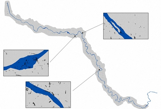
The rasters produced in the eCognition-based automated method for extracting LWD indicated whether each pixel contained LWD of no LWD; Figure 4 shows an example of this output at the Cedar River. The LiDAR estimated surface area is compared to the field measured surface area for the Cedar River plots in Figure 5. A simple, no-intercept linear model was fit to these data, yielding a slope of 0.55 and a coefficient of determination of 0.83. This model was used to predict the field measured surface area at the Raging, Snoqualmie, and Green Rrivers (Figure 6). The model was biased toward under-predicting LWD surface area (slope of 2.10) but the model did explain 64% of the variability. A comparison of the LiDAR estimated surface area to the field measured surface area using data from all of the plots measured in this study was also conducted (Figure 7), explaining 65% of the variability.

3.2. LWD Identification, Manual Method

The delineation of LWD by the trained interpreter using LiDAR alone required 2 h and 55 min, while the delineation using imagery alone required 2 h and 2 min. The added detail of combining LiDAR and imagery required 9 h and 32 min. It was obvious that the most detail was provided by utilizing both the imagery and LiDAR, thus, subsequent accuracy assessments utilized this dataset only. A map using the same extents as Figure 2 of the manual LWD identification using LiDAR and imagery is displayed in Figure 8. An accuracy assessment was performed using a simiple linear regression comparing the summed lengths of all of the LWD within the extent of each Cedar River plot using both field-measured and manually-delineated LWD. Manually-identified LWD only explained 36% of the variability observed in field-measured LWD. It was likely that this relatively poor correlation was a result of small pieces of LWD identified manually but not identified in the field due to the restriction on not counting LWD with a maximum diameter smaller than 30.5 cm. Thus, we filtered the manually-identified LWD dataset by progressively removing shorter LWD in increments of 1 m. At each incremental step, a linear regression was performed comparing field-measured LWD to manually-measured LWD. Figure 9 displays the change in the coefficient of determination from this regression with each incremental step, up to a maximum increment of LWD greater than 25 m in length. A local maximum was reached at 18 m, at which point 76% of the variability in field measured LWD was explained (Figure 10). We conluded that a filter of 18 m represented the best match between the field-measured LWD length and the manually-delineated LWD.

3.3. Individual Tree Identification

The IT classification for the Cedar River is shown in Figure 11; classifications for the other four river systems are not shown, but all 25 IT plots are used in the subsequent analysis described below. We attempted to compare field-measured tree heights to the maximum height of each canopy object, but the results showed no correlation (r² < 0.01). Additional analysis (not shown) suggested that errors in the GPS combined with the leaf-off condition made accurate comparison impossible; thus, we chose to examine the IT accuracy at a plot level by treating each image object as a potential clump of multiple trees and focusing only on larger trees that could become recruitable LWD. Figure 12 shows the total area of all image objects in the 20–30 m and 30 m and greater classes as compared to the number of trees taller than 20 m in height measured in the field for each plot explaining 47% of the variability.

4. Discussion

4.1. Automated Versus Manual Identification of LWD

The two methods of mapping the presence of LWD produce accurate results, but differ in their utility and applicability. We showed that the automated process using eCognition can provide accurate results at the Cedar River (Figure 5), but the model developed from the Cedar River was biased when applied to the other watersheds (Figure 6). A likely explanation for this bias is the small sample size () used in building the model using the Cedar River plots. Plots with large quantities of LWD also negatively affect the accuracy. This is likely due to large wood accumulations, which we discuss in more detail below. A benefit of the automated approach is that it can be rapidly applied over large areas, allowing for watershed level analyses of LWD distribution. The limitation is that it is not possible to extract individual pieces of LWD from the automated analysis, as the raster result is only a pixel by pixel estimation of the presence of LWD. As such, there is no way to measure the length of LWD or count the number of pieces present. The manual analysis showed similar accuracy to the automated analysis when filtering for LWD length, but is more time consuming to apply over large areas. The benefit of the manual analysis is that it allows for measuring the length of individual pieces of LWD and allows a tidier map to be produced. Previous studies have come to similar conclusions about LWD detection in non-riparian forest environments [18]. Another caveat to interpreting our results is that we did not randomly assign plots across the landscape and, thus, we do not have plots that contain little or no LWD. Future studies should include these plots in their field campaigns.

4.2. Large Wood Accumulations

Large wood accumulations (LWA), also known as log jams, are a difficult problem for both field measurement and remote sensing techniques. The LWA form when individual pieces of LWD become entangled during a period of high river flow. It is impossible to count and measure every piece of LWD during a field survey because many pieces are buried. In addition, the LWA contains many small pieces of LWD and a large amount of sediment and non-woody organic material. Figure 13 shows an example of a LWA at the Cedar River. The red lines represent the best attempt by the image interpreter to identify individual pieces, but it is clear that there are many smaller pieces that cannot be resolved. The eCognition algorithm also struggles with LWA because their shape and size are so different from the linear, individual LWA spread across the landscape. These results agree with previous research that found that eCognition-based algorithms struggled at identifying downed logs in forest environments when logs were too close together [18]. One solution may be to categorize LWA differently than individual pieces of LWD, focusing and the surface area or volume of the LWA and using an allometric relationship to estimate the number of LWD within the LWA. Building these allometric equations would require further field research.

4.3. Strengths and Limitations of the Individual Tree Analysis

The IT analysis failed to delineate individual trees that could be verified using field data, but it was moderately successful at estimating the number of larger trees within a plot. This relatively low accuracy seen in Figure 12 is likely caused by the leaf-off LiDAR data. Most of the trees in the plots were deciduous, although a few evergreen conifers were included. The leaf-off conditions aided the LWD analysis, but restricted the accuracy of the IT analysis. The high spatial precision of the mapped tree clumps (Figure 11) is the strength of the analysis, though, because it allows the interpreters of these data to know an estimated number of large trees within a specific distance of the river, which is pertinent to the recommendations below. Previous studies have shown much better accuracies when delineating and assessing the number of large trees in forested environments, suggesting that the results of this method could have been much more accurate given leaf-on LiDAR data [20,21,22,23].

4.4. Recommendations for Integrated Monitoring and Future Research

The results of this study present two datasets (LWD and IT) that can be used together to produce an estimate of the number of contemporary and recruitable LWD. As noted above, the spatial positioning of the modeled individual trees is useful for managers seeking to understand the risk of adding additional LWD becoming recruited during a period of high flow. For instance, King County managers classify land areas in the flood zone near the main flow of the river as areas at high risk for channel migration. If the river changes course during a flood event, the individual trees within this channel migration zone (CMZ) are likely to become LWD. The high population near the rivers used in this study requires a good understanding of both the potential risks of LWD impacting residences and infrastructure while balancing the ecological benefits An example analysis is presented in Figure 14 showing how the results of this study can be used to produce a map of tree density and, thus, recruitment risk for the Cedar River. The figure shows the density of model estimated trees greater than 20 m tall and near enough to the river that if a tree fell it could potentially span at least half the distance of the width of the river. Tree density is only shown for areas in the CMZ. Density is displayed using existing polygons that King County uses as river management units. The information in Figure 14, in conjunction with Figure 4 and Figure 8, can help to provide the integrated assessment of contemporary and recruitable LWD by highlighting areas of highest risk for managers.

Future research could improve on these methods by utilizing higher resolution LiDAR and imagery to better identify smaller LWD. Methods should also be developed to better manage the complications imposed by LWA, with one possibility being the development of allometric equations based on surface area or volume. LiDAR and imagery taken in both leaf-on and leaf-off conditions could also maximize the accuracies of estimating both LWD and individual trees.

5. Conclusions

In this study, we have demonstrated an integrated approach for monitoring contemporary and recruitable LWD using remotely-sensed data. We demonstrated an automated method for quantifying LWD using aerial LiDAR and object-based image analysis techniques, as well as a manual method for quantifying LWD using image interpretation derived from LiDAR rasters and aerial four-band imagery. In addition, we employed an established method for estimating the number of individual trees within the riparian forest. These methods, when compared to field data, showed high accuracies for the LWD method and moderate accuracy for the individual tree method. These methods can be rapidly deployed by managers for quantifying the risk and benefits of LWD in river ecosystems, increasing the tools available for managers to make difficult decisions, such as when and where to remove standing trees. Additional research and higher detail remotely-sensed datasets are required to refine and increase the accuracy of these methods to better quantify contemporary and recruitable LWD across a wide range of heterogeneous environments.

References

1. Abbe, T.B.; Montgomery, D.R. Large woody debris jams, channel hydraulics and habitat formation in large rivers. Regul. Rivers Res. Manag. 1996, 12, 201–221. [Google Scholar] [CrossRef]
2. Sollins, P. Input and decay of coarse woody debris in coniferous stands in western Oregon and Washington. Can. J. For. Res. Revue Can. Rech. For. 1982, 12, 18–28. [Google Scholar] [CrossRef]
3. Angermeier, P.L.; Karr, J.R. Relationships between woody debris and fish habitat in a small warmwater stream. Trans. Am. Fish. Soc. 1984, 113, 716–726. [Google Scholar] [CrossRef]
4. Beechie, T.J.; Sibley, T.H. Relationships between channel characteristics, woody debris, and fish habitat in northwestern Washington streams. Trans. Am. Fish. Soc. 1997, 126, 217–229. [Google Scholar] [CrossRef]
5. Moulin, B.; Piegay, H. Characteristics and temporal variability of large woody debris trapped in a reservoir on the River Rhone (Rhone): Implications for river basin management. River Res. Appl. 2004, 20, 79–97. [Google Scholar] [CrossRef]
6. Mazzorana, B.; Comiti, F.; Volcan, C. Determining flood hazard patterns through a combined stochastic-deterministic approach. Nat. Hazards 2011, 59, 301–316. [Google Scholar] [CrossRef]
7. Schmocker, L.; Hager, W.H. Probability of drift blockage at bridge. Decks. J. Hydraul. Eng. 2011, 137, 470–479. [Google Scholar] [CrossRef]
8. Biedenweg, K.; Akyuz, K.; Skeele, R. Balancing riparian management and river recreation: methods and applications for exploring floater behavior and their interaction with large wood. Environ. Manag. 2012, 50, 283–295. [Google Scholar] [CrossRef] [PubMed]
9. Schuett-Hames, D.; Pleus, A.E.; Ward, J.; Fox, M.; Light, J. TFW Monitoring Program Method Manual for the Large Woody Debris Survey; Washington Department of Natural Resources: Olympia, WA, USA, 1999. [Google Scholar]
10. Leckie, D.G.; Cloney, E.E.; Jay, C.; Paradine, D. Automated mapping of stream features with high-resolution multispectral imagery: An. example of the capabilities. Photogramm. Eng. Remote Sens. 2005, 71, 145–155. [Google Scholar] [CrossRef]
11. Marcus, W.A.; Legleiter, C.J.; Aspinall, R.J.; Boardman, J.W.; Crabtree, R.L. High spatial resolution hyperspectral mapping of in-stream habitats, depths, and woody debris in mountain streams. Geomorphology 2003, 55, 363–380. [Google Scholar] [CrossRef]
12. Marcus, W.A.; Marston, R.A.; Colvard, C.R., Jr.; Gray, R.D. Mapping the spatial and temporal distributions of woody debris in streams of the Greater Yellowstone Ecosystem, USA. Geomorphology 2002, 44, 323–335. [Google Scholar] [CrossRef]
13. Smikrud, K.M.; Prakash, A. Monitoring large woody debris dynamics in the Unuk River, Alaska using digital aerial photography. Gisci. Remote Sens. 2006, 43, 142–154. [Google Scholar] [CrossRef]
14. Pasher, J.; King, D.J. Mapping dead wood distribution in a temperate hardwood forest using high resolution airborne imagery. For. Ecol. Manag. 2009, 258, 1536–1548. [Google Scholar] [CrossRef]
15. Eamer, J.B.R.; Walker, I.J. Quantifying sand storage capacity of large woody debris on beaches using LiDAR. Geomorphology 2010, 118, 33–47. [Google Scholar] [CrossRef]
16. Pesonen, A.; Maltamo, M.; Kangas, A. The comparison of airborne laser scanning-based probability layers as auxiliary information for assessing coarse woody debris. Int. J. Remote Sens. 2010, 31, 1245–1259. [Google Scholar] [CrossRef]
17. Mucke, W.; Deák, B.; Schroiff, A.; Hollaus, M.; Pfeifer, N. Detection of fallen trees in forested areas using small footprint airborne laser scanning data. Can. J. Remote Sens. 2013, 39, S32–S40. [Google Scholar] [CrossRef]
18. Blanchard, S.D.; Jakubowski, M.K.; Kelly, M. Object-Based image analysis of downed logs in disturbed forested landscapes using LiDAR. Remote Sens. 2011, 3, 2420–2439. [Google Scholar] [CrossRef]
19. Nystrom, M.; Holmgren, J.; Fransson, J.E.S.; Olsson, H. Detection of windthrown trees using airborne laser scanning. Int. J. Appl. Earth Obs. Geoinf. 2014, 30, 21–29. [Google Scholar] [CrossRef]
20. Richardson, J.J.; Moskal, L.M. Strengths and limitations of assessing forest density and spatial configuration with aerial LiDAR. Remote Sens. Environ. 2011, 115, 2640–2651. [Google Scholar] [CrossRef]
21. Reitberger, J.; Schnörr, C.; Krzystek, P.; Stilla, U. 3D segmentation of single trees exploiting full waveform LiDAR data. ISPRS J. Photogramm. Remote Sens. 2009, 64, 561–574. [Google Scholar] [CrossRef]
22. Hirata, Y.; Furuya, N.; Suzuki, M.; Yamamoto, H. Airborne laser scanning in forest management: Individual tree identification and laser pulse penetration in a stand with different levels of thinning. For. Ecol. Manag. 2009, 258, 752–760. [Google Scholar] [CrossRef]
23. Andersen, H.E. Using airborne Light Detection and Ranging (LiDAR) to characterize forest stand. condition on the Kenai Peninsula of Alaska. West. J. Appl. For. 2009, 24, 95–102. [Google Scholar]
Figure 1. (A) shows Washington State with King County in grey and the study area location as a black dot (47.482878, −122.217066); (B) shows the four river systems and the extent of remotely sensed data coverage; (C) shows an example of a large wood plot (location shown by * in B); and (D) shows an example of an individual tree plot (location shown by + in B).
Remotesensing 08 00778 g001
Figure 2. Histogram of individual tree diameters at breast height (DBH) in all individual tree (IT) plots.
Remotesensing 08 00778 g002
Figure 3. Histogram of individual tree heights in all individual tree (IT) plots.
Remotesensing 08 00778 g003
Figure 4. Map of LWD for Cedar River using the automated method.
Remotesensing 08 00778 g004
Figure 5. Comparison of automated LWD detection to field-surveyed LWD at Cedar River.
Remotesensing 08 00778 g005
Figure 6. Model-predicted LWD as compared to field-measured LWD at Green, Raging, and Snoqualmie Rivers.
Remotesensing 08 00778 g006
Figure 7. Comparison of model-predicted LWD detection to field-measured LWD at all rivers.
Remotesensing 08 00778 g007
Figure 8. Map of LWD for Cedar River using the manual method with imagery and LiDAR combined.
Remotesensing 08 00778 g008
Figure 9. Amount of variability explained by model predicting field-measured LWD length from manually-identified LWD length when the minimum length for inclusion in the model is reduced from 0–25 m.
Remotesensing 08 00778 g009
Figure 10. Assessment of accuracy of manual LWD identification when compared to field-surveyed LDW with a minimum length of 18 m at Cedar River.
Remotesensing 08 00778 g010
Figure 11. Map of individual and clumped trees for Cedar River.
Remotesensing 08 00778 g011
Figure 12. Accuracy of individual tree frequency estimation using LiDAR-based methods for trees greater than 20 m in height.
Remotesensing 08 00778 g012
Figure 13. LWD from a Cedar River plot. Red lines are manually-identified LWD.
Remotesensing 08 00778 g013
Figure 14. Example of LWD recruitment potential in high risk areas.
Remotesensing 08 00778 g014