Application of Convolution Neural Networks and Hydrological Images for the Estimation of Pollutant Loads in Ungauged Watersheds


Abstract
:1. Introduction
2. Materials and Methods
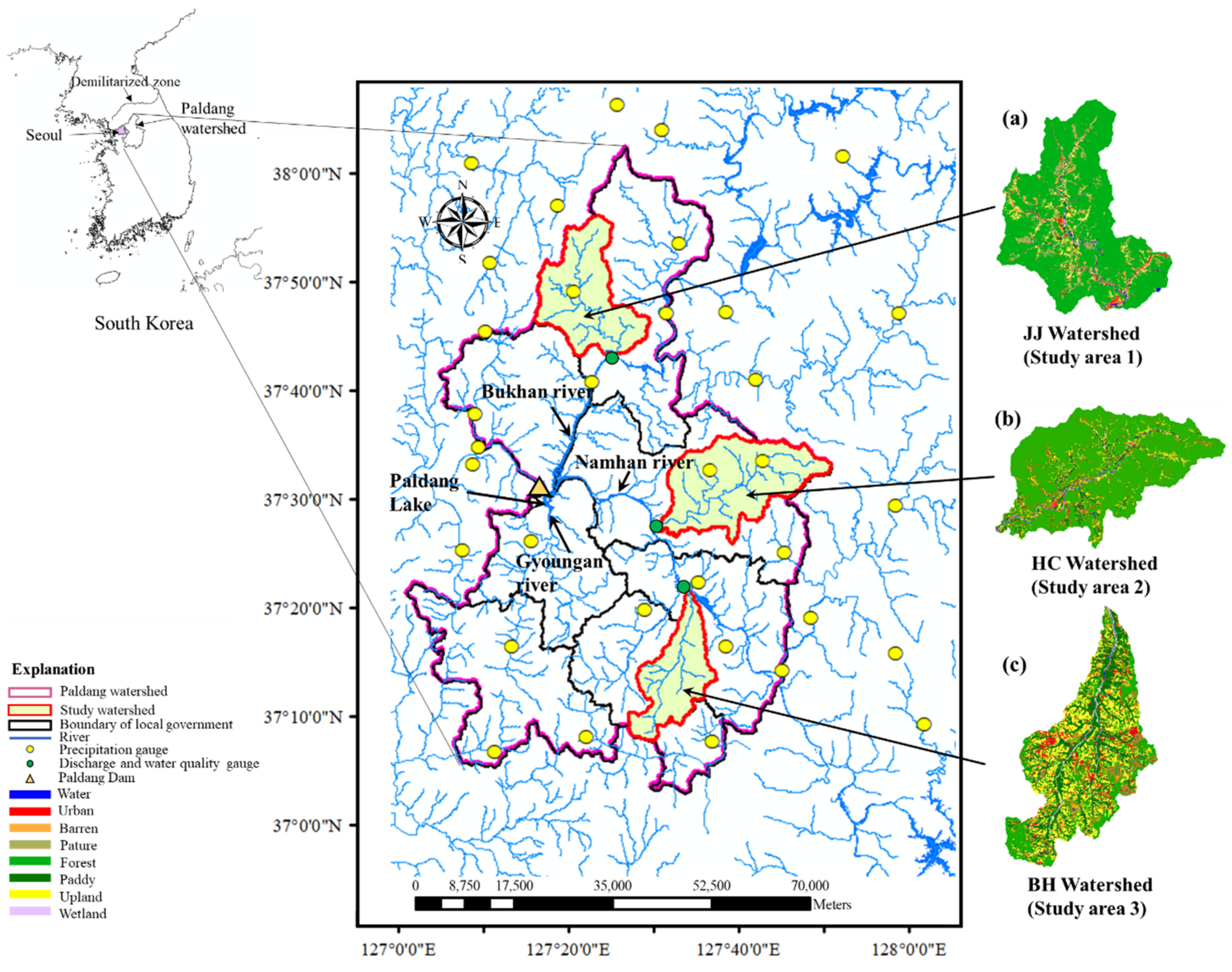
2.1. Study Area
2.2. Data for the Study
2.2.1. Data Collection
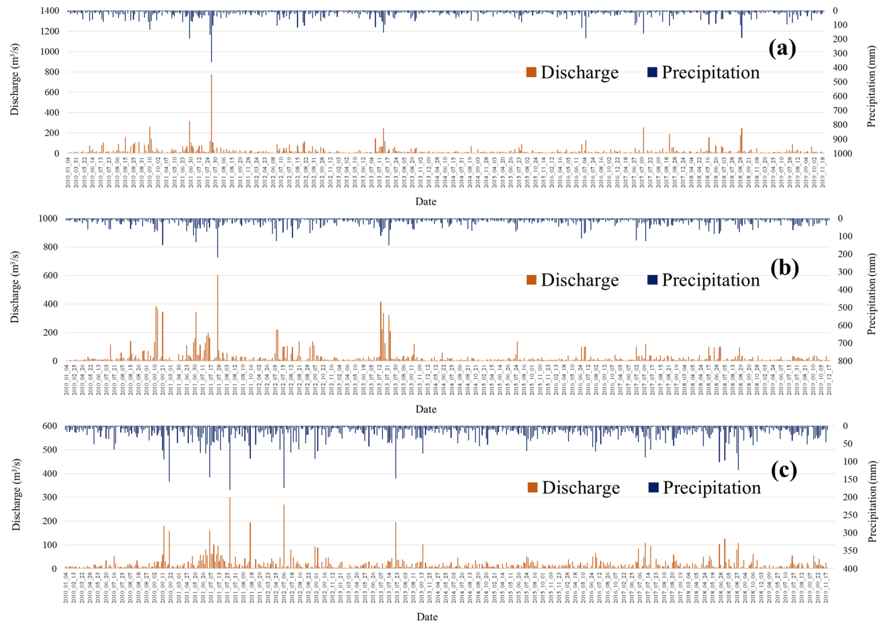
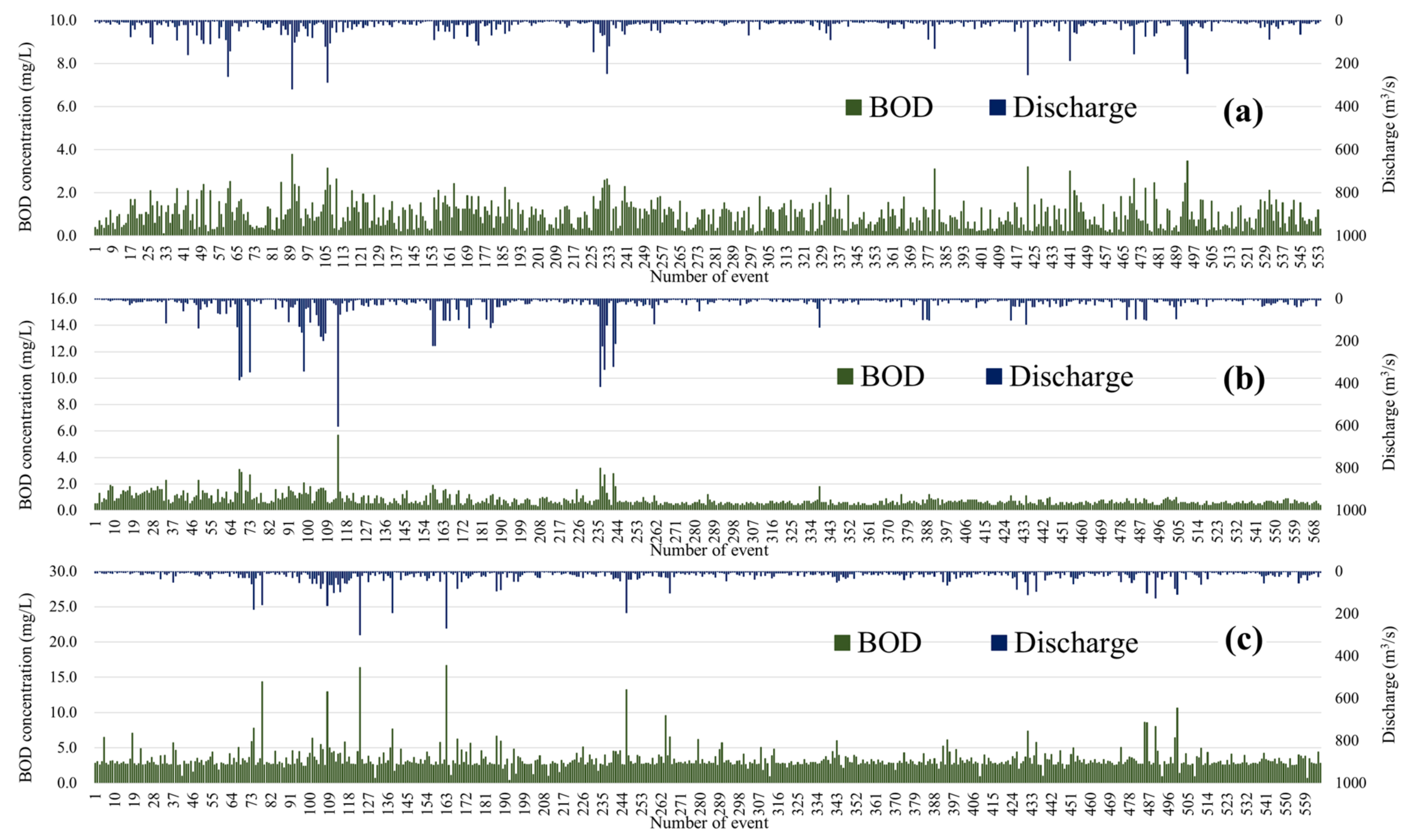
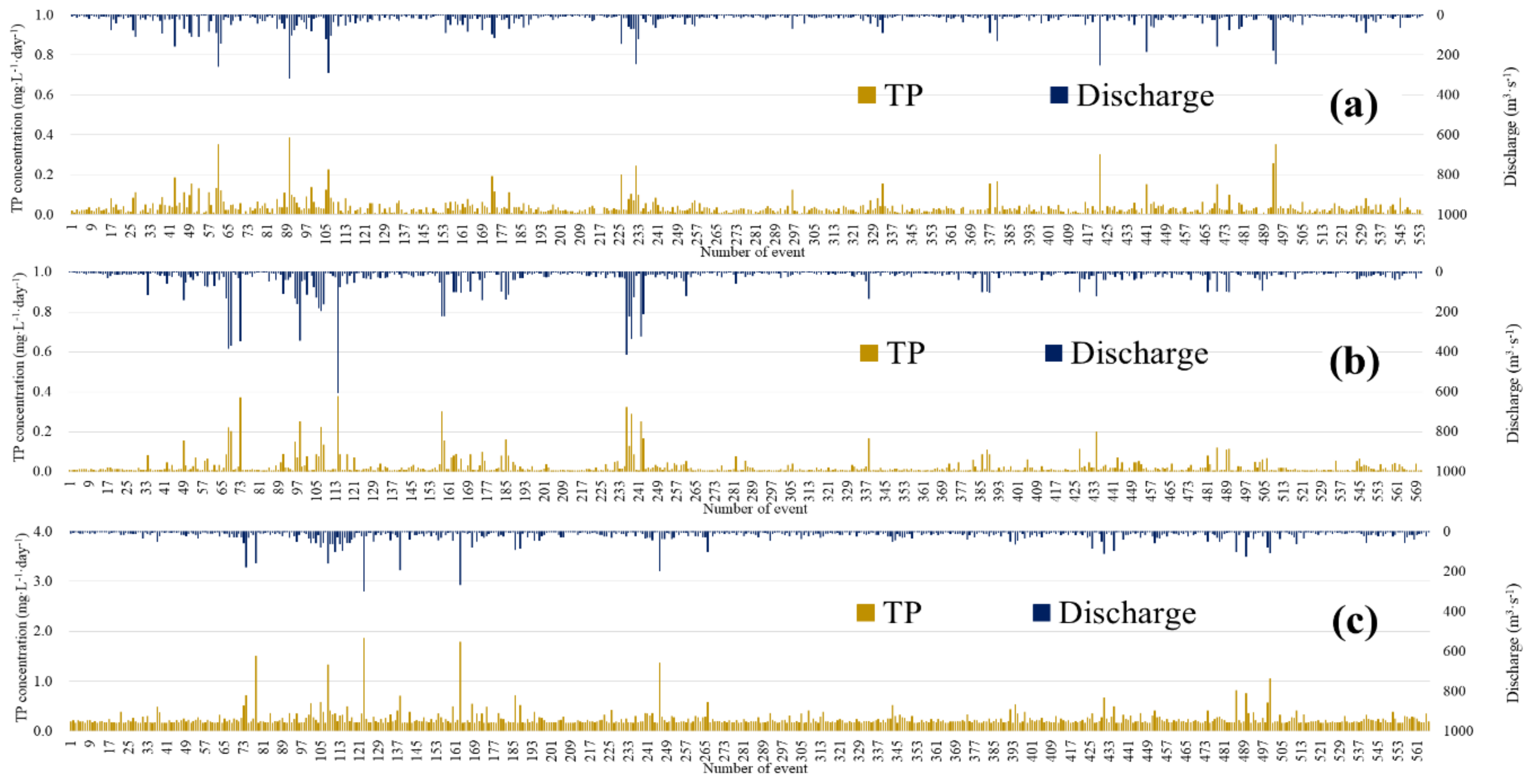
2.2.2. Data during the Study Period
2.3. Research Method
2.3.1. CNN Model Dataset
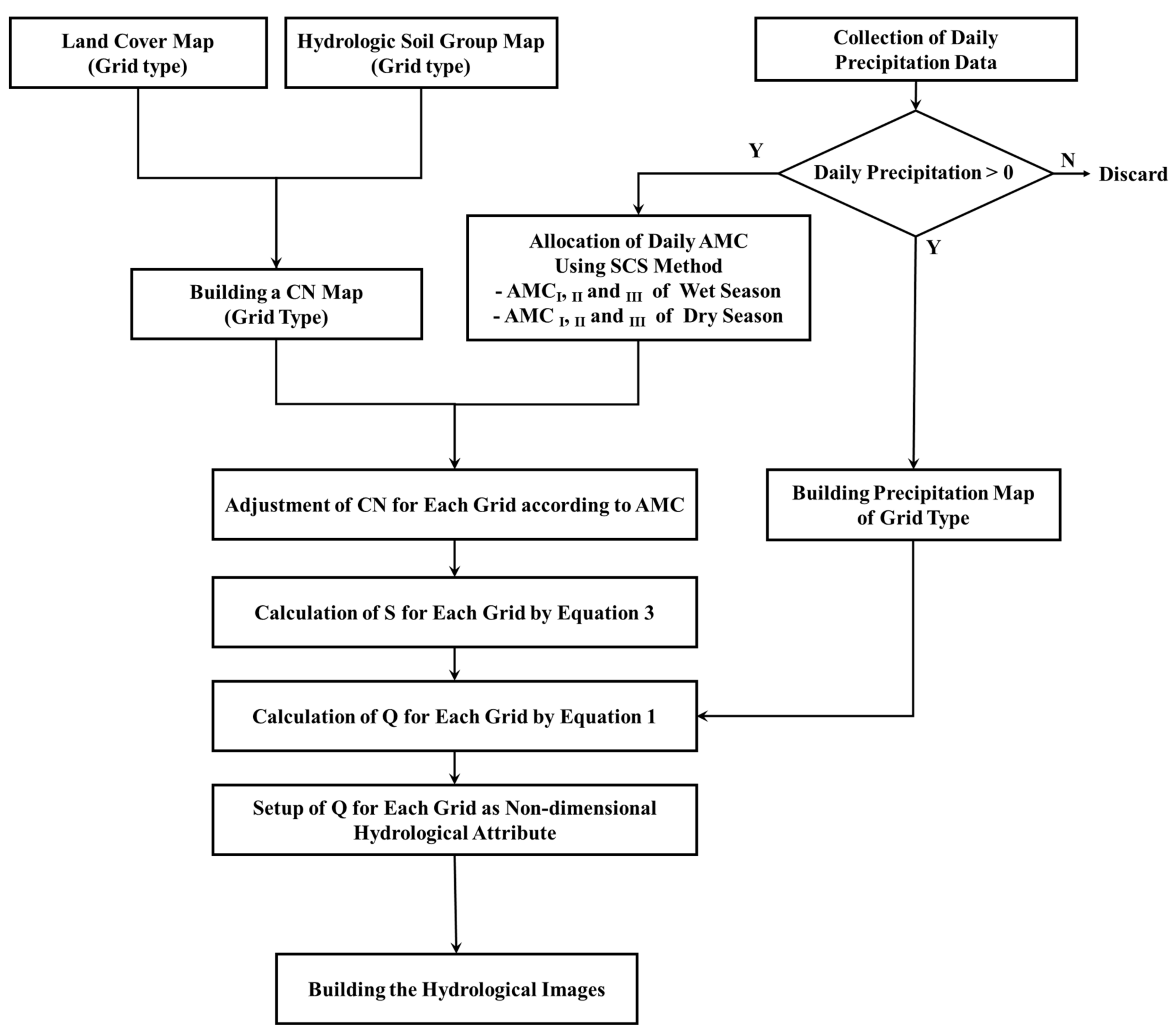
- Building a Hydrological Image as a Feature for CNN Model Training
- 2.
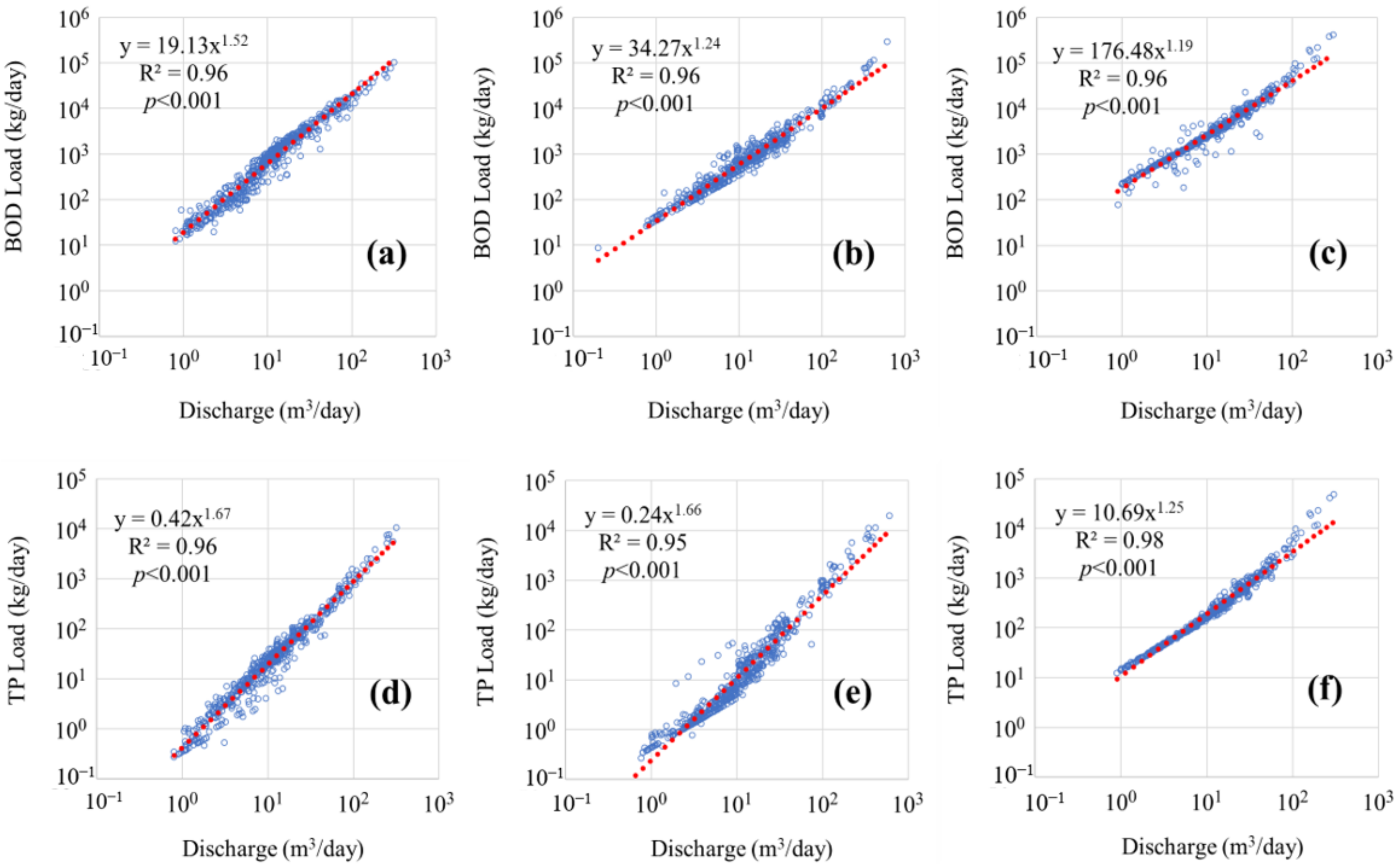
- Building Target Data
- 3.
- Establishing the Dataset for CNN Model Training and Testing
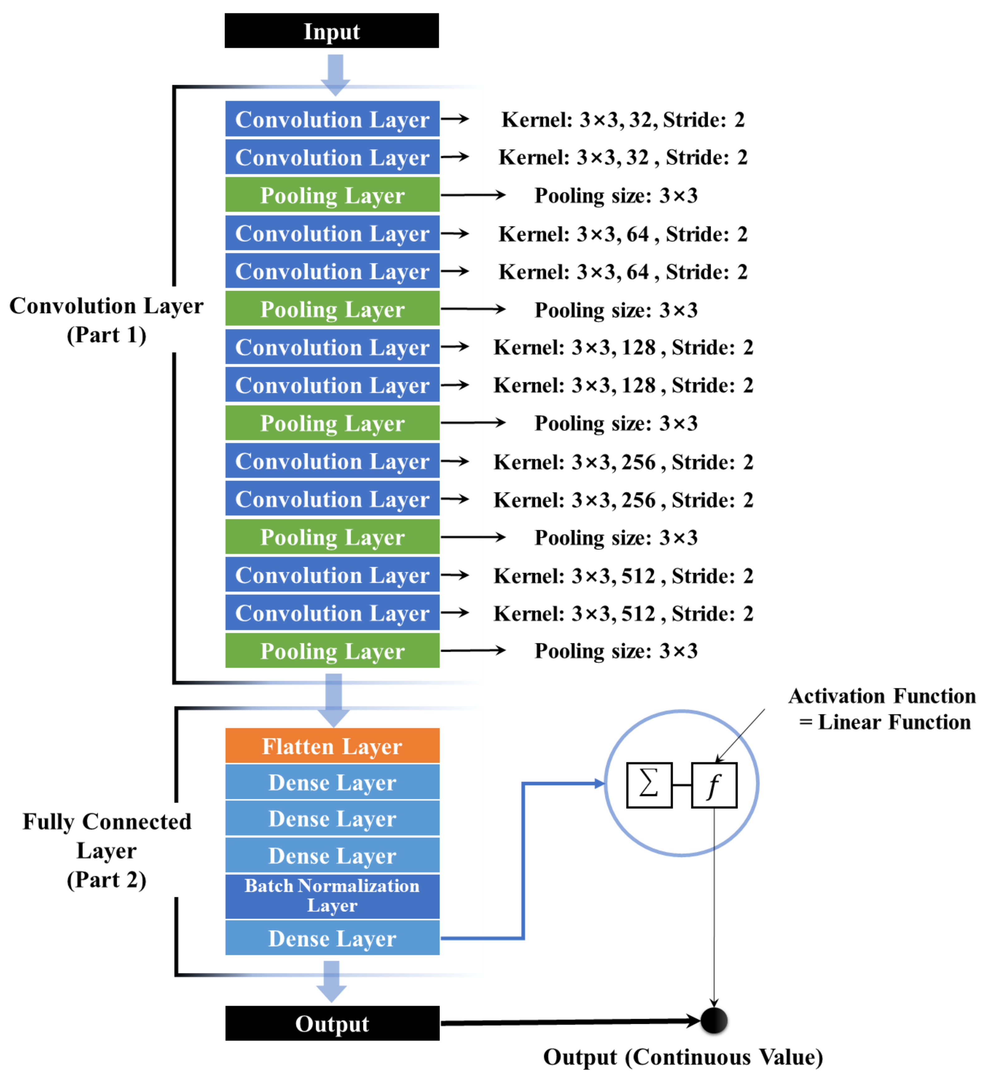
2.3.2. CNN Model Structure
2.3.3. Hyper-Parameter Setting of the CNN Model
2.4. Evaluation of the CNN Model
3. Results and Discussion
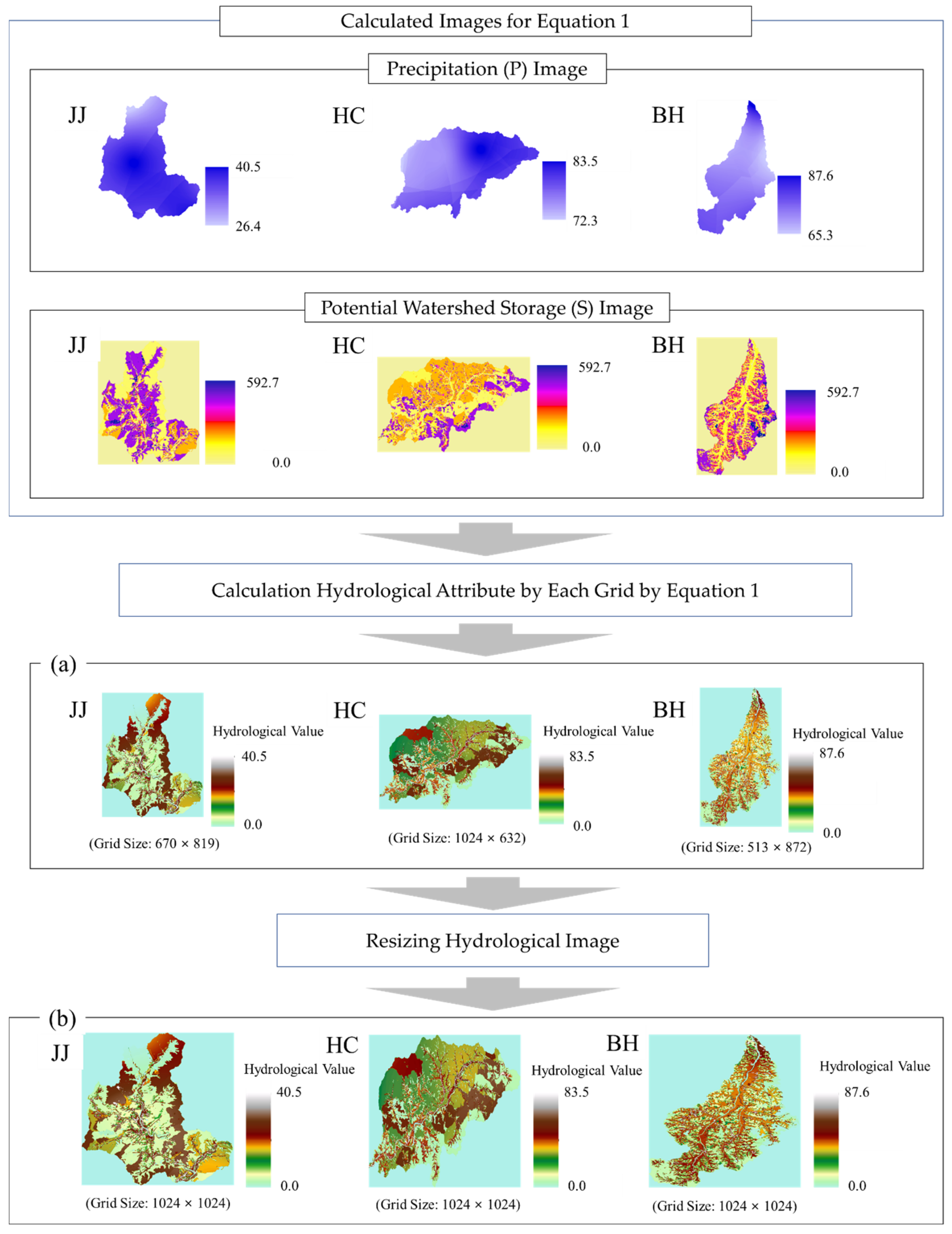
3.1. Hydrological Image Generation and Image Datasets Construction Results
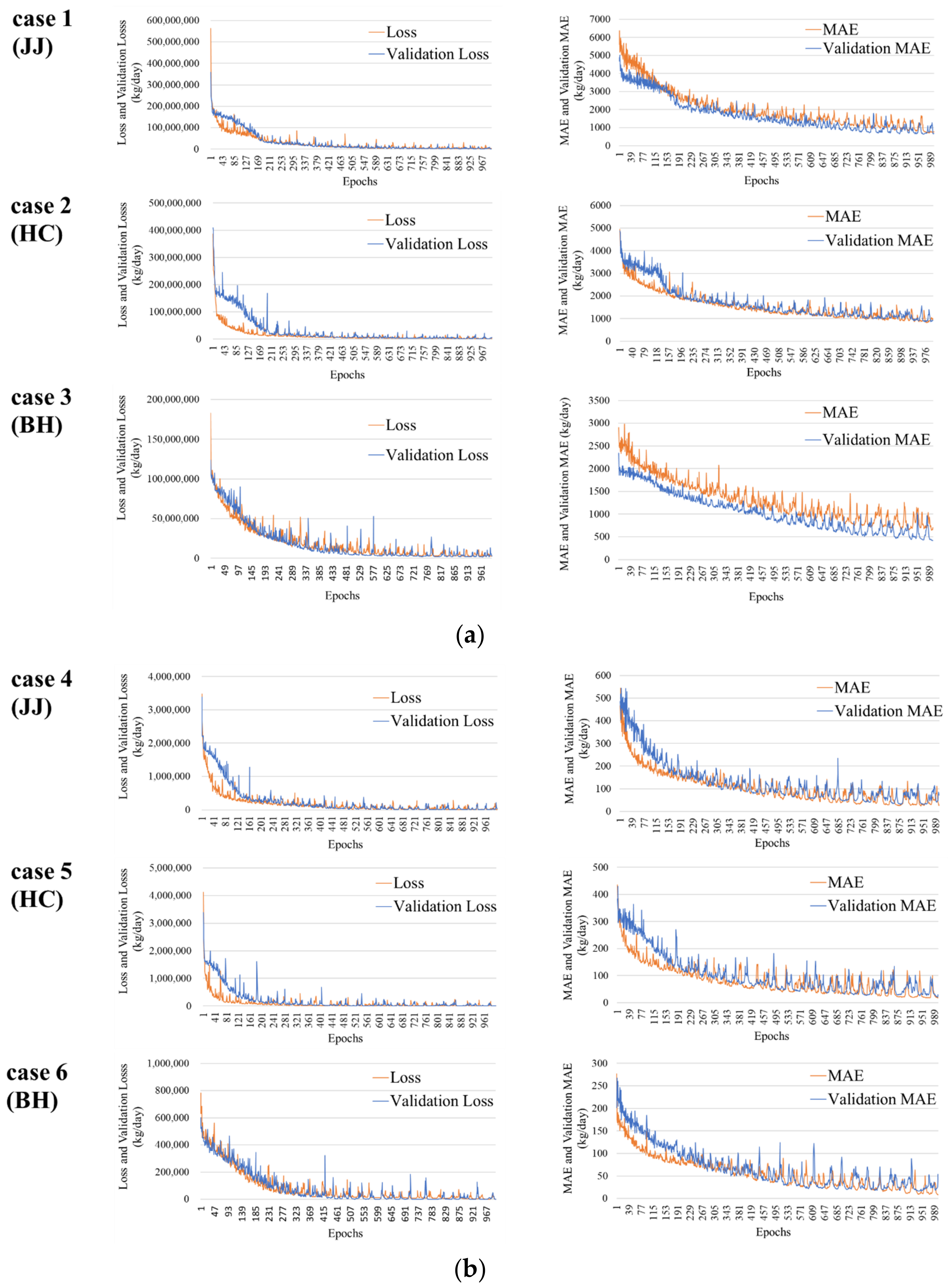
3.2. CNN Model Architecture and Training Results
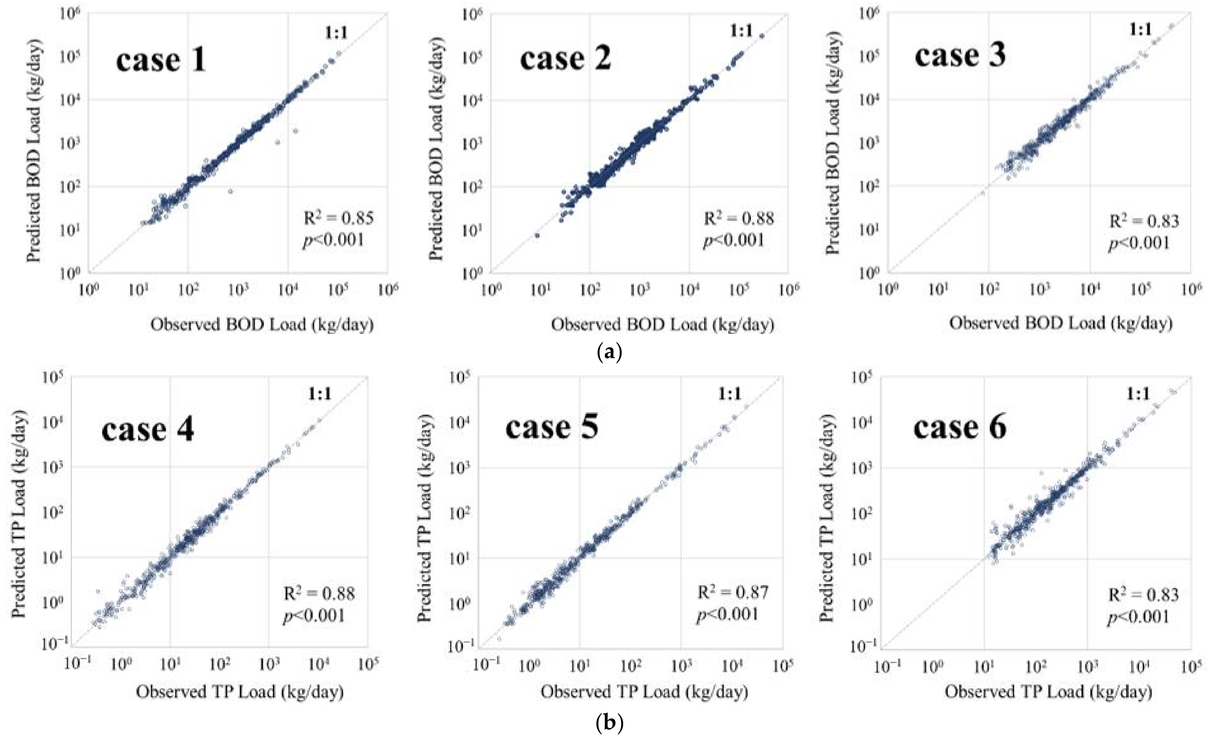
3.3. Prediction Results of the CNN Model and Model Evaluation
4. Conclusions
Funding
Institutional Review Board Statement
Informed Consent Statement
Data Availability Statement
Conflicts of Interest
References
- Young, R.A.; Onstad, C.A.; Bosch, D.D.; Anderson, W.P. AGNPS: A nonpoint source pollution model for evaluating agricultural watersheds. J. Soil Water Conserv. 1989, 44, 168–173. [Google Scholar]
- Arnold, J.G.; Allen, P.M.; Bernhardt, G. A comprehensive surface-groundwater flow model. J. Hydrol. 1993, 142, 47–69. [Google Scholar] [CrossRef]
- Lewis, A.R. Storm Water Management Model User’s Manual; Water Supply and Water Resources Division National Risk Man-agement Research Laboratory: Cincinnati, OH, USA, 2004. [Google Scholar]
- Aisha, M.S. Evaluation of SWAT Model Applicability for Water Impairment Identification and TMDL Analysis. Ph.D. Thesis, University of Maryland, College Park, MD, USA, 30 October 2007. [Google Scholar]
- Patel, A.B.; Joshi, G.S. Modeling of rainfall-runoff correlations using artificial neural network-a case study of dharoi watershed of a sabarmati river basin, India. Civ. Eng. J. 2017, 3, 78–87. [Google Scholar] [CrossRef]
- Song, C.M.; Kim, J.S. Applicability evaluation of the hydrological image and convolution neural network for prediction of the biochemical oxygen demand and total phosphorus loads in agricultural areas. Agriculture 2020, 10, 529. [Google Scholar] [CrossRef]
- Mercier, G.; Blais, J.F.; Chartier, M. Décontamination à l’échelle pilote de sols pollués en métaux toxiques par des procédés miniers et lixiviation chimique. J. Environ. Eng. Sci. 2007, 6, 53–64. [Google Scholar] [CrossRef]
- Salas, F.R.; Somos-Valenzuela, M.A.; Dugger, A.; Maidment, D.R.; Gochis, D.J.; David, C.H.; Yu, W.; Ding, D.; Clark, E.P.; Noman, N. Towards real-time continental scale streamflow simulation in continuous and discrete space. JAWRA J. Am. Water Resour. Assoc. 2018, 54, 7–27. [Google Scholar] [CrossRef]
- Akhtar, M.K.; Corzo, G.A.; van Andel, S.J.; Jonoski, A. River flow forecasting with artificial neural networks using satellite observed precipitation pre-processed with flow length and travel time information: Case study of the Ganges river basin. Hydrol. Earth Syst. Sci. 2009, 13, 1607–1618. [Google Scholar] [CrossRef] [Green Version]
- Cakir, S.; Sita, M. Evaluating the performance of ANN in predicting the concentrations of ambient air pollutants in Nicosia. Atmos. Pollut. Res. 2020, 11, 2327–2334. [Google Scholar] [CrossRef]
- Kiiza, C.; Pan, S.; Bockelmann-Evans, B.; Babatunde, A. Predicting pollutant removal in constructed wetlands using artificial neural networks (ANNs). Water Sci. Eng. 2020, 13, 14–23. [Google Scholar] [CrossRef]
- Hamed, M.M.; Khalafallah, M.G.; Hassanien, E.A. Prediction of wastewater treatment plant performance using artificial neural networks. Environ. Model. Softw. 2004, 19, 919–928. [Google Scholar] [CrossRef]
- Mishra, P.K.; Karmakar, S. Performance of optimum neural network in rainfall–runoff modeling over a river basin. Int. J. Environ. Sci. Technol. 2018, 16, 1289–1302. [Google Scholar] [CrossRef]
- Pradhan, P.; Tingsanchali, T.; Shrestha, S. Evaluation of soil and water assessment tool and artificial neural network models for hydrologic simulation in different climatic regions of Asia. Sci. Total Environ. 2020, 701, 13–144. [Google Scholar] [CrossRef] [PubMed]
- Rajaee, T.; Khani, S.; Ravansalar, M. Artificial intelligence-based single and hybrid models for prediction of water quality in rivers: A review. Chemom. Intell. Lab. Syst. 2020, 200, 103978. [Google Scholar] [CrossRef]
- Zhu, S.; Heddam, S. Prediction of dissolved oxygen in urban rivers at the Three Gorges Reservoir, China: Extreme learning machines (ELM) versus artificial neural network (ANN). Water Qual. Res. J. 2019, 55, 106–118. [Google Scholar] [CrossRef]
- Wilby, R.L.; Abrahart, R.; Dawson, C. Detection of conceptual model rainfall—runoff processes inside an artificial neural network. Hydrol. Sci. J. 2003, 48, 163–181. [Google Scholar] [CrossRef] [Green Version]
- Jain, A.; Sudheer, K.P.; Srinivasulu, S. Identification of physical processes inherent in artificial neural network rainfall runoff models. Hydrol. Process. 2004, 18, 571–581. [Google Scholar] [CrossRef]
- Sudheer, K.P.; Jain, A. Explaining the internal behaviour of artificial neural network river flow models. Hydrol. Process. 2004, 18, 833–844. [Google Scholar] [CrossRef]
- Biswas, A.K. Integrated water resources management: A reassessment. Water Int. 2004, 29, 248–256. [Google Scholar] [CrossRef]
- EGIS: Environmental Geographic Information Service. Available online: https://www.egis.me.go.kr (accessed on 9 January 2019).
- WAMIS: Water Management Information System, National Institute of Environmental Research. Available online: https://www.water.nier.go.kr (accessed on 1 March 2019).
- KMA: Korea Meteorological Administration. Available online: https://www.kma.go.kr (accessed on 3 January 2020).
- NIER: National Institute of Environmental Research. Available online: https://www.nier.go.kr (accessed on 11 November 2019).
- Song, C.M. Hydrological image building using curve number and prediction and evaluation of runoff through convolution neural network. Water 2020, 12, 2292. [Google Scholar] [CrossRef]
- United States Department of Agriculture; Natural Resources Conservation Service (NRCS); Conservation Engineering Division. Urban Hydrology for Small Watersheds; Natural Resources Conservation Service: Washington, DC, USA, 1986. Available online: https://www.nrcs.usda.gov/Internet/FSE_DOCUMENTS/stelprdb1044171.pdf (accessed on 2 November 2019).
- Li, C.; Liu, M.; Hu, Y.; Shi, T.; Zong, M.; Walter, M.T. Assessing the impact of urbanization on direct runoff using improved composite cn method in a large urban area. Int. J. Environ. Res. Public Health 2018, 15, 775. [Google Scholar] [CrossRef] [Green Version]
- Wang, H.; Chen, Y. Identifying key hydrological processes in highly urbanized watersheds for flood forecasting with a distributed hydrological model. Water 2019, 11, 1641. [Google Scholar] [CrossRef] [Green Version]
- Ministry of Land, Infrastructure and Transport. Design Flood Estimation Techniques; Ministry of Land Transport and Maritime Affairs: Seoul, Korea, 2012. (In Korean)
- Schumann, A.H. Thiessen polygon. In Encyclopedia of Hydrology and Lakes. Encyclopedia of Earth Science; Springer: Dordrecht, The Netherlands, 1998; pp. 648–649. [Google Scholar] [CrossRef]
- Miller, H. Tobler’s first law and spatial analysis. Ann. Assoc. Am. Gerogr. 2004, 94, 284–289. [Google Scholar] [CrossRef]
- Python. Available online: https://www.python.org/ (accessed on 4 January 2020).
- LeCun, Y.; Bottou, L.; Bengio, Y.; Haffner, P. Gradient-based learning applied to document recognition. IEEE 1998, 86, 2278–2324. [Google Scholar] [CrossRef] [Green Version]
- Taravat, A.; Del Frate, F.; Cornaro, C.; Vergari, S. Neural networks and support vector machine algorithms for automatic cloud classification of whole-sky ground-based images. IEEE Trans. Geosci. Remote Sens. Lett. 2014, 12, 666–670. [Google Scholar] [CrossRef]
- Medina, E.; Petraglia, M.R.; Gomes, J.G.R.C.; Petraglia, A. Comparison of CNN and MLP classifiers for algae detection in underwater pipelines. In Proceedings of the 2017 Seventh International Conference on Image Processing Theory, Tools and Applications (IPTA), Montreal, QC, Canada, 28 November–1 December 2017; pp. 1–6. [Google Scholar]
- Zeiler, M.D.; Fergus, R. Visualizing and understanding convolutional networks. In Computational Data and Social Networks; Springer Science and Business Media LLC: Berlin, Germany, 2014; Volume 8689, pp. 818–833. [Google Scholar]
- Ide, H.; Kurita, T. Improvement of learning for CNN with ReLU activation by sparse regularization. In Proceedings of the 2017 International Joint Conference on Neural Networks (IJCNN), Anchorage, AK, USA, 14–19 May 2017; pp. 2684–2691. [Google Scholar]
- Chen, Z.; Ho, P.-H. Global-connected network with generalized ReLU activation. Pattern Recognit. 2019, 96, 106961. [Google Scholar] [CrossRef]
- Keras. The Python Deep Learning API. Available online: https://keras.io/ (accessed on 27 August 2020).
- TensorFlow. An End-to-End Open Source Machine Learning Platform. Available online: https://www.tensorflow.org/ (accessed on 27 August 2020).
- Bottou, L. Large-scale machine learning with stochastic gradient descent. In Proceedings of the 19th International Conference on Computational Statistics, Paris, France, 22–27 August 2010; pp. 177–186. [Google Scholar] [CrossRef] [Green Version]
- Qian, N. On the momentum term in gradient descent learning algorithms. Neural Netw. 1999, 12, 145–151. [Google Scholar] [CrossRef]
- Nesterov, Y. A method for unconstrained convex minimization problem with the rate of convergence. Doklady USSR 1983, 269, 543–547. Available online: https://www.semanticscholar.org/paper/A-method-for-unconstrained-convex-minimization-with-Nesterov/ed910d96802212c9e45d956adaa27d915f5d7469 (accessed on 18 April 2020).
- Duchi, J.; Hazan, E.; Singer, Y. Adaptive subgradient methods for online learning and stochastic optimization. JMLR 2011, 12, 2121–2159. [Google Scholar]
- Dozat, T. Incorporating nesterov momentum into Adam. In Proceedings of the ICLR Workshop, San Juan, Puerto Rico, 2–4 May 2016; pp. 2013–2016. Available online: https://openreview.net/pdf/OM0jvwB8jIp57ZJjtNEZ.pdf (accessed on 21 April 2020).
- Zeiler, M.D. ADADELTA: An Adaptive Learning Rate Method. arXiv 2012, arXiv:1212.5701v1. [Google Scholar]
- Hinton, G.; Tieleman, T. RMSprop Gradient Optimization. Lecture 6e of his Coursera Class. 2014. Available online: https://www.cs.toronto.edu/~{}tijmen/csc321/slides/lecture_slides_lec6.pdf (accessed on 10 February 2019).
- Kingma, D.P.; Ba, J. Adam: A method for stochastic optimization. In Proceedings of the International Conference Learnning Representations (ICLR), San Diego, CA, USA, 5–8 May 2015. [Google Scholar]
- Pillow. Available online: https://www.python-pillow.org (accessed on 10 February 2020).
- Lee, K.; Choi, C.; Shin, D.H.; Kim, H.S. Prediction of heavy rain damage using deep learning. Water 2020, 12, 1942. [Google Scholar] [CrossRef]
- Alsumaiei, A.A. Utility of artificial neural networks in modeling pan evaporation in hyper-arid climates. Water 2020, 12, 1508. [Google Scholar] [CrossRef]
- Mulualem, G.M.; Liou, Y.-A. Application of artificial neural networks in forecasting a standardized precipitation evapotranspiration index for the upper blue nile basin. Water 2020, 12, 643. [Google Scholar] [CrossRef] [Green Version]
- Dancey, C.; Reidy, J. Statistics without Maths for Psychology, 5th ed.; Prentice Hall: Upper Saddle River, NJ, USA, 2011. [Google Scholar]
- Lipiwattanakarn, S.; Saengsawang, S. Performance comparison of a conceptual hydrological model and a back-propagation neural network model in rainfall-runoff modeling. Eng. J. Res. Dev. 2005, 16, 35–42. [Google Scholar]
- Azadi, S.; Amiri, H.; Rakhshandehroo, G.R. Evaluating the ability of artificial neural network and PCA–M5P models in predicting leachate COD load in landfills. Waste Manag. 2016, 55, 220–230. [Google Scholar] [CrossRef] [PubMed]
- Yu, T.; Yang, S.; Bai, Y.; Gao, X.; Li, C. Inlet water quality forecasting of wastewater treatment based on kernel principal component analysis and an extreme learning machine. Water 2018, 10, 873. [Google Scholar] [CrossRef] [Green Version]
- Yan, J.; Xu, Z.; Yu, Y.; Xu, H.; Gao, K. Application of a hybrid optimized bp network model to estimate water quality parameters of beihai lake in beijing. Appl. Sci. 2019, 9, 1863. [Google Scholar] [CrossRef] [Green Version]
- Shao, D.; Nong, X.; Tan, X.; Chen, S.; Xu, B.; Hu, N. Daily water quality forecast of the south-to-north water diversion project of china based on the cuckoo search-back propagation neural network. Water 2018, 10, 1471. [Google Scholar] [CrossRef] [Green Version]


| Study Area | Land Cover | |||||||||
|---|---|---|---|---|---|---|---|---|---|---|
| Water | Urban | Barren | Pasture | Forest | Paddy | Upland | Wetland | Total | ||
| JJ Watershed (Study area 1) | Area (km2) | 2.6 | 5.8 | 5.2 | 19.2 | 207.5 | 4.4 | 13.5 | 2.4 | 260.6 |
| Proportion (%) | 1.0 | 2.2 | 2.0 | 7.4 | 79.6 | 1.7 | 5.2 | 0.9 | 100.0 | |
| HC Watershed (Study area 2) | Area (km2) | 2.3 | 6.5 | 2.9 | 22.5 | 235.8 | 20.8 | 19.6 | 3.7 | 314.1 |
| Proportion (%) | 0.7 | 2.1 | 0.9 | 7.2 | 75.1 | 6.6 | 6.2 | 1.2 | 100.0 | |
| BH Watershed (Study area 3) | Area (km2) | 1.6 | 11.7 | 4.0 | 18.2 | 41.6 | 50.9 | 49.7 | 3.5 | 181.1 |
| Proportion (%) | 0.9 | 6.5 | 2.2 | 10.1 | 23.0 | 28.1 | 27.4 | 1.9 | 100.0 | |
| Model | Image Data | Target Data | Dataset Classification |
|---|---|---|---|
| Case 1 | Hydrological images of HC and BH | BOD Load of HC and BH | Input Dataset |
| Hydrological images of JJ | BOD Load of JJ | Test Dataset | |
| Case 2 | Hydrological images of JJ and BH | BOD Load of HC and BH | Input Dataset |
| Hydrological images of HC | BOD Load of JJ | Test Dataset | |
| Case 3 | Hydrological images of JJ and HC | BOD Load of HC and BH | Input Dataset |
| Hydrological images of BH | BOD Load of JJ | Test Dataset | |
| Case 4 | Hydrological images of HC and BH | TP Load of HC and BH | Input Dataset |
| Hydrological images of JJ | TP Load of JJ | Test Dataset | |
| Case 5 | Hydrological images of JJ and BH | TP Load of JJ and BH | Input Dataset |
| Hydrological images of HC | TP Load of HC | Test Dataset | |
| Case 6 | Hydrological images of JJ and HC | TP Load of JJ and HC | Input Dataset |
| Hydrological images of BH | TP Load of BH | Test Dataset |
| Model | Target | Dataset | Number of Data | Note | |
|---|---|---|---|---|---|
| Case 1 | BOD Load | Input Dataset | Training Dataset | 796 | HC–BH |
| Validation Dataset | 341 | HC–BH | |||
| Test Dataset | Test Dataset | 554 | JJ (Entire study period) | ||
| Case 2 | Input Dataset | Training Dataset | 784 | JJ–BH | |
| Validation Dataset | 336 | JJ–BH | |||
| Test Dataset | Test Date Set | 571 | HC (Entire study period) | ||
| Case 3 | Input Dataset | Training Dataset | 788 | HC–JJ | |
| Validation Dataset | 337 | HC–JJ | |||
| Test Dataset | Test Date Set | 566 | BH (Entire study period) | ||
| Case 4 | TP Load | Input Dataset | Training Dataset | 796 | HC–BH |
| Validation Dataset | 341 | HC–BH | |||
| Test Dataset | Test Date Set | 554 | JJ (Entire study period) | ||
| Case 5 | Input Dataset | Training Dataset | 784 | JJ–BH | |
| Validation Dataset | 336 | JJ–BH | |||
| Test Dataset | Test Date Set | 571 | HC (Entire study period) | ||
| Case 6 | Input Dataset | Training Dataset | 788 | HC–JJ | |
| Validation Dataset | 337 | HC–JJ | |||
| Test Dataset | Test Date Set | 566 | BH (Entire study period) | ||
| Convolution Layer | Output Shape (Raw_Size, Column_Size, Image_Channel) | Number of Parameter | Activation Function |
| Conv2D 1 | 507, 507, 32 | 320 | ReLu |
| Conv2D 2 | 254, 254, 32 | 9248 | |
| MaxPooling 1 | 127, 127, 32 | 0 | |
| Conv2D 3 | 64, 64, 64 | 18,496 | ReLu |
| Conv2D 4 | 64, 64, 64 | 36,928 | |
| MaxPooling 2 | 32, 32, 64 | 0 | |
| Conv2D 5 | 32, 32, 128 | 73,856 | ReLu |
| Conv2D 6 | 32, 32, 128 | 147,584 | |
| MaxPooling 3 | 16, 16, 128 | 0 | |
| Conv2D 7 | 16, 16, 256 | 295,168 | ReLu |
| Conv2D 8 | 16, 16, 256 | 590,080 | |
| MaxPooling 4 | 8, 8, 256 | 0 | |
| Conv2D 9 | 8, 8, 512 | 1,180,160 | ReLu |
| Conv2D 10 | 8, 8, 512 | 2,359,808 | |
| MaxPooling_5 | 4, 4, 512 | 0 | |
| Fully Connected Layer | Output Shape (Number of Node) | Parameter | Activation Function |
| Flatten Layer | 8192 | 0 | |
| Dense Layer 1 | 1024 | 8,389,632 | ReLu |
| Dense Layer 2 | 1024 | 1,049,600 | ReLu |
| Dense Layer 3 | 1024 | 1,049,600 | ReLu |
| Batch Normalization Layer | 1024 | 4096 | ReLu |
| Dense Layer 4 | 1 | 1025 | Liner |
| Contents | Target | Predicted Study Area | r | NSE | RMSE (kg·day−1) | MAPE (%) |
|---|---|---|---|---|---|---|
| Case 1 | BOD Load | JJ (Study Area 1) | 0.92 | 0.90 | 1031.1 | 11.5 |
| Case 2 | HC (Study Area 1) | 0.94 | 0.92 | 1152.2 | 15.9 | |
| Case 3 | BH (Study Area 1) | 0.91 | 0.84 | 5376.5 | 20.1 | |
| Case 4 | TP Load | JJ (Study Area 1) | 0.94 | 0.93 | 53.6 | 17.9 |
| Case 5 | HC (Study Area 1) | 0.93 | 0.91 | 169.5 | 16.3 | |
| Case 6 | BH (Study Area 1) | 0.90 | 0.84 | 476.5 | 21.3 |
Publisher’s Note: MDPI stays neutral with regard to jurisdictional claims in published maps and institutional affiliations. |
© 2021 by the author. Licensee MDPI, Basel, Switzerland. This article is an open access article distributed under the terms and conditions of the Creative Commons Attribution (CC BY) license (http://creativecommons.org/licenses/by/4.0/).
Share and Cite
Song, C.M. Application of Convolution Neural Networks and Hydrological Images for the Estimation of Pollutant Loads in Ungauged Watersheds. Water 2021, 13, 239. https://doi.org/10.3390/w13020239
Song CM. Application of Convolution Neural Networks and Hydrological Images for the Estimation of Pollutant Loads in Ungauged Watersheds. Water. 2021; 13(2):239. https://doi.org/10.3390/w13020239
Chicago/Turabian StyleSong, Chul Min. 2021. "Application of Convolution Neural Networks and Hydrological Images for the Estimation of Pollutant Loads in Ungauged Watersheds" Water 13, no. 2: 239. https://doi.org/10.3390/w13020239
APA StyleSong, C. M. (2021). Application of Convolution Neural Networks and Hydrological Images for the Estimation of Pollutant Loads in Ungauged Watersheds. Water, 13(2), 239. https://doi.org/10.3390/w13020239