A Quick Survey of the Most Vulnerable Areas of a Water Distribution Network Due to Transients Generated in a Service Line: A Lagrangian Model Based on Laboratory Tests

Abstract

This paper analyses the propagation and mechanisms of interaction of a pressure wave in a looped water distribution network by means of laboratory and numerical tests. Transients are generated by the complete and fast closure of a valve, simulating an end-user maneuver, located at the downstream end section of a service line. The adequate length of the service line allows capturing each single pressure wave inserted into the network. The executed tests and successive analysis by means of a Lagrangian model (LM) highlight the effect of the network topology and the location of the transient generation point but in a more expeditious way with respect to the use of a complete transient model. The most excited part of the system is the one in close proximity of the end-user and then the corresponding service line. Within the network, pressure waves accumulate in the areas with the smallest diameter pipes. By means of the refined LM—which is able to capture the pressure extreme values occurring in the first phases of the transient—the vulnerability maps of the network are provided. Such maps identify the nodes subjected to the most severe pressure waves in terms of both frequency and amplitude. The exposure level to transients of each node is synthesized by the value of the vulnerability index proposed in this paper.

1. Introduction

Until a few years ago, the effects of transients would have been considered a marginal problem in the management of Water Distribution Networks (WDNs). Such a conviction comes from some commonly accepted—perhaps uncritically—assumptions that, as discussed below, are being questioned today. The first one is to assume WDNs as self-protected against transient events because of the large number of simultaneously active users, each of them being a “natural” way out of pressure waves from the WDN. The second assumption is to attribute the large number of faults occurring in the small diameter pipes to their less accurate installation and larger number of connections—each of them being a potential weak point—with respect to the large diameter ones. The third one is to ascribe the pipe stress and related bursts and leakage to the large value of the steady-state pressure regime and/or to large, even if infrequent, overpressures caused by, as an example, pump switch-off. As an example, in [1] the role of the high pressure values is shown to be correlated to the frequency of pipe breaks. In accordance with such assumptions, in most cases the only preventive action is the installation of pressure reducing valves (e.g., [2,3]).

In many cases, it is arduous identifying the actual cause of a large leakage affecting only some parts of a WDN that exhibit no clear differences from other parts in terms of pipe material, maintenance, or pressure (that is usually monitored at low frequencies).

A possible explanation of such a feature could derive from a proper identification of the nature of the actually dangerous transients and the different exposure the individual parts of the considered WDN has to them. It is quite arduous for the water utility companies to suppress all leaks or prevent all pressure variations in WDNs. They usually install conventional surge protection devices (e.g., air vessel) in the main pipes to damp the more extreme pressure variations (e.g., the ones due to pump failure). However, the sources may be within the plumbing systems of the end-users and out of the regulatory control of the water utilities [4]. In fact, transients generated by users’ consumption variations may be dangerous because of their very high frequency [5]: such small, but incessant, pressure changes can, in fact, increase the failure rate [6,7]. Furthermore, the frequent occurrences of transients due to the daily pump operation for system management can result in the deterioration of infrastructure safety and life cycles in the long term [8]. In [9], this aspect has been discussed by numerical tests and a multi-objective optimization framework has been developed for the optimal WDN design.

Numerical experiments executed in [10] within a Monte Carlo simulation-based approach investigate the effect of the uncertainty due to natural or human behaviors that actually affects the value of some parameters—e.g., wave speed, pipe diameter, and friction—usually considered as known inputs in traditional water hammer models. Of particular interest for real pipe systems is the uncertainty of the air component—pointed out successively by the experiments carried out in [11]—that affects the value of the pressure wave speed and then pressure extreme values. The First-Order-Second-Moment-based analysis method and numerical applications are then used in [12] for a sensitivity study of a transient frequency response method to the different influence factors (e.g., initial and boundary conditions) in multiple-pipeline systems with simple branched and looped pipe junctions.

In transient simulations, a further potential source of uncertainty is the nodal demand transformation within system skeletonization [13]. The peculiarities of transients that require the adoption of different skeletonization rules with respect to steady-state conditions are pointed out in [14]. As an example, the effect of the dead ends is null in steady-state conditions, whereas they lock pressure waves into the system in a cumulative fashion [15,16].

The impact of the demand modelling method—an issue recognized as crucial since the pioneering paper by [17]—on the performance of the hydraulic model of WDNs is examined in [18]. In this paper, the performance of the extended period simulation (EPS) is compared with the one of the “complete” unsteady flow model for elastic pipes—i.e., the model based on the Method of Characteristics [19] with the unsteady friction [20,21] and viscoelastic effects [22] included —taken as a benchmark. The results of the executed numerical experiments show that the use of the EPS along with a demand deterministic approach produces large errors in terms of both pressure and discharge transient response. On the contrary, the quality of the numerical simulations improves if a demand stochastic approach is followed. The much better performance of the “complete” unsteady flow model with respect to the EPS is confirmed by the results of the numerical tests provided in [23].

In order to discern when to apply which type of model, the need to balance computational efficiency with physical accuracy in the modelling of transients in WDNs is addressed in several papers where the results of the “complete” unsteady flow model, rigid water column-based model, and EPSs are compared [24,25,26]. The subject remains challenging and under debate even if innovative approaches—e.g., of a hybrid type [27]—are emerging.

For several reasons, less attention has been devoted to laboratory and field experiments. The lack of space, the large number of possible combinations of loops (e.g., number, diameter distribution, and layout) make more attractive, also from an economic point of view, numerical experiments with respect to the laboratory ones. The need of monitoring a large number of sections in terms of not only pressure but also discharge—to control the users’ random water consumption and all boundary conditions—makes the execution of significant tests in real WDNs very arduous. Specifically, only three papers offered contributions on the laboratory side: two papers aimed at localizing transient sources [28] and leaks [29] in a very small diameter network. In addition, the recent contribution by [30] examined the transient response of a small network consisting of six 3 × 3 m square loops with polymeric pipes. Because of the characteristics of the used laboratory setup—particularly the small length of the pipes—in the acquired pressure signals, the mechanisms of propagation of the single pressure waves in the network, as a result of the system layout, cannot be analyzed in detail. As is evident, no papers explicitly studied the end-user’s effect and the mechanism of propagation of pressure waves in a looped laboratory network that can be representative of a real WDN. Only in [31,32], laboratory experiments considered a service line and partially concerned the effect of water consumption variations. Specifically, in [31] six transients were generated on a tree network both in the main pipe and within the plumbing system, with the aim of pointing out the possible occurrence of negative pressures and related back-flow phenomena in the plumbing system. Pressure was only measured in the plumbing systems. In [32], transients were generated in the main pipes to check the effect on the service lines in terms of leaks.

The contribution on field tests side is slightly larger [4,7,33,34,35,36,37]. However, in such papers, transients were generated in the supply lines and/or their effects were studied in the main pipes. Moreover, as specifically highlighted by [17,37], a more rigorous field test program is necessary for understanding the widespread occurrence of transients in complex WDNs. Very few papers analyze the effect of water consumption variations. In [5], the results of the monitoring and analysis of the transient response of a real WDN subjected to the changes of the users’ water consumption are presented. The analysis highlights that the pressure signals are characterized by long-term changes (low-frequency) on which shorter period (high-frequency) ones overlap. The long-term oscillations are linked to the topological and mechanical characteristics of the network, whereas the high-frequency pressure ones are related to user activity changes. In [38], the mentioned field pressure signals are simulated by means of a “complete” numerical model within an innovative stochastic approach. Precisely, the generated water consumption scenarios at a 1 s time step with random manoeuvre times allow properly reproducing the main pressure statistics (i.e., mean, variance, and extreme values) of the observed transient response.

In conclusion, very few tests were executed both in the laboratory and in the field to analyze the effect of water consumption variations in both the service line and the main pipes. These tests do not allow drawing general conclusions and do not highlight the role of the network topology or the location of the transient generation point. To fill this gap, this paper aims to give a contribution to the analysis of the mechanism of propagation of a pressure wave in a looped network (two 100 × 100 m square loops) with one active service line but in different locations. Accordingly, experiments have been carried out at the Water Engineering Laboratory (WEL) of the University of Perugia, Italy. During tests, the pressure signals (i.e., the time history of the pressure head) have been acquired in several measurement sections located both in the main pipes and the service line. Moreover, the laboratory layout has been designed to be representative of a real WDN: the two loops consist of pipes of different diameters, and the considered water consumption variation is consistent with the typical consumption of sanitary appliances [39]. In addition, thanks to the adequate length of the service line (=23.6 m), the behavior of each single pressure wave has been captured [14]. The experimental results have been examined by means of a Lagrangian model (LM). The aim of these tests is to point out the most excited part of the system, both in the main pipe and in the service line, according to the different location of the transient generation point. Moreover, the effect of the topology of the network has been analyzed in detail to evaluate its effect on the amplitude of transients. The LM is first used to interpret the experimental data, and, since it is able to capture the extreme values of pressure in the first phases of the transient tests, it is then used to build a map of the most excited parts of the network.

The organization of this paper is as follows. Section 2 begins with a description of the experimental setup and the preliminary tests executed to characterize the end-user and service line. This section also introduces a brief breakdown of the laboratory transient tests, and the LM used to interpret the laboratory data. The effect of the network topology and the transient generation point is highlighted and discussed in Section 3 and Section 4, respectively. Successively, a procedure for implementing the map of vulnerability that points out the parts of the network more exposed to transient effects, is described. Finally, conclusions are drawn in Section 6.

2. Materials and Methods

2.1. The Experimental Setup

The experimental setup (Figure 1a) at the Water Engineering Laboratory (WEL) of the University of Perugia, Italy is a pipe network with two loops—indicated as I and II—simulating a District Metered Area (DMA). All pipes are high density polyethylene (HDPE) pipes and are supplied by a tank pressurized by a pump, with a shut-off head of 2.4 bar. A pipe with a length L = 42.3 m, internal diameter, D = 93.3 mm, nominal diameter DN110, and wall thickness e = 8.1 mm connects the supply tank to the DMA. All the pipes of the two loops have a length L = 100 m. Loop I has four main pipes with D = 63.8 mm, DN75, and e = 5.6 mm. One of the four main pipes of loop II is in common with loop I, whereas the other three have D = 42.6 mm, DN50, and e = 3.7 mm.

In order to simulate the user’s service line, a branch (L = 23.6 m, D = 20 mm, DN25, and e = 3 mm) has been alternatively installed at nodes 5 (Figure 1a), 6, and 7, respectively. At the downstream end of such a branch (i.e., at nodes 5u, 6u, and 7u), a solenoid valve in series with a ball valve is installed to simulate the end-user (Figure 1b). Specifically, the ball valve equipped with a protractor to check the actual opening degree allows simulating different water consumptions. In addition, the solenoid valve generates controlled, repeatable, and sharp transients for simulating changes of the end-user consumption. As an example, Figure 1c indicates the location of the measurement sections around junction 5 (shown in Figure 1d). In addition to node 5, very close to the junction pressure signals are also acquired at nodes $5_8$, $5_4$, and $5_6$ located 1 m from junction 5 along the three main pipes connected to it (with the subscript indicating the closest node). In all configurations, the supplied steady-state discharge is measured at node 2 located at a distance of 22.2 m from the tank by means of a magnetic flow meter. Pressure is monitored at nodes 4, 5, 6, 7, and 8 and at the measurement sections (Figure 1a) denoted with two numbers indicating the closest and farthest junction, respectively. For the sake of clarity, 32 indicates the measurement section located at a distance of 8.4 m from junction 3 (the closest one) and 11.7 m from junction 2 (the farthest one). Finally, each junction connected to the service line has been fully monitored by adding a measurement section at a distance of 1 m in each main pipe connected to it. During tests, pressures are sampled at a frequency of 2048 Hz by a National Instrument cDAQ-9188 data acquisition system. Relative (G) piezoresistive pressure transducers have been installed with a full scale ($fs$) variable from 6 bar G to 10 bar G in the network. To capture eventual relative negative pressure in the service line, absolute (A) piezoresistive transducers are used from 15 bar A to 16 bar A. All these transducers have an accuracy of 0.25% $fs$. For all tests, the water temperature is quite constant and equal to about 18 °C.

2.2. Preliminary Tests for the End-User and Service Line Characterization

In order to characterize the end-user and service line, some preliminary tests have been executed. Firstly, the ball valve at the end-user has been geometrically characterized. Precisely, the relationship between the valve relative opening $\varphi$ ($\varphi$ = 0 for fully closed valve and $\varphi$ = 1 for fully open valve) and dimensionless cross-sectional area $A_v/A$—with $A_v$ = ball valve cross-sectional area, and A = pipe area—has been obtained by means of a 3D AutoCAD model and checked by a photographic analysis. Figure 2a shows the good agreement between such a geometric relationship and the results by [40].

Secondly, steady-state tests have been carried out for evaluating the end-user hydraulic characteristics. Precisely, the local head loss, $\zeta$, across the two installed in series valves has been measured for different values of $\varphi$ and discharge, Q.

According to the usual flow conditions in real pipe systems, experiments concerned turbulent flow with values of the Reynolds number that ranges from 6700 to 183,000. Accordingly, for any given relative opening, $\varphi$, the constant value of the in series valve effective area ($C_{sv}{A}_{sv}$) has been determined by means of the following equation:

$$Q=C_{sv}{A}_{sv}\sqrt{2g\zeta }$$

(1)

with $A_{sv}$ ($C_{sv}$) = in series valve area (discharge coefficient), and g = gravity acceleration. Figure 2b shows the experimental hydraulic characteristics of the end-user—i.e., the relationship between $\varphi$ and $C_{sv}{A}_{sv}/A$)—and the corresponding fitting function ($C_{sv}{A}_{sv}/A=0.802{\varphi }^2-0.035\varphi$).

Further preliminary experiments allowed evaluating the pressure wave speed, a, of both the network pipes and service line by measuring the pressure wave travel time. As a result, the following values have been obtained: $a_{DN25}$ = 455.91 m/s, $a_{DN50}$ = 379.81 m/s, $a_{DN75}$ = 387.89 m/s, and $a_{DN110}$ = 398.82 m/s, all compatible with the geometrical and mechanical characteristics of the pipes.

2.3. Laboratory Transient Tests

Table 1. Main characteristics of the executed laboratory tests.

Test No. (#)	Layout	Maneuver Type	Discharge [L/s]
1	service line connected at node 5	Total closure of 5u	$Q_{0,5u}$ = 0.12
2	service line connected at node 6	Total closure of 6u	$Q_{0,6u}$ = 0.12
3	service line connected at node 7	Total closure of 7u	$Q_{0,7u}$ = 0.12

shows the main characteristics of the tests carried out at WEL. The aim of these tests is to analyze the effect of the topology and location of the pressure waves generation point on the network transient response. Accordingly, the executed tests differ for the network layout, boundary conditions, and water consumption at the end-user, $Q_{0,yu}$, with the subscripts 0 and $yu$ indicating the steady-state conditions and the end-user (with y = 5, 6, and 7, alternately), respectively. To emphasize the dynamic response of the system, transients have been generated by the complete and fast closure of the valve located at the downstream end section of the service line. This manoeuvre simulates actions initiated within a house such as the manual closure of a tap or the automatic shut off of the solenoid valve of the washing machine. As a consequence, the variation of the discharge generating the overpressure, $\Delta Q_{yu}$, is equal to $Q_{0,yu}$. Specifically, tests with $Q_{0,yu}$ = 0.12 L/s are considered since this value is consistent with the typical consumption of sanitary appliances [39] and does not cause water column separation phenomena [32]. During tests #1, #2, and #3, the end-user 5u, 6u, and 7u is almost instantaneously closed, respectively. During these tests, the network is fully closed; in other words, no further users are open, except valves at the end-users 5u, 6u, and 7u, respectively.

2.4. The Lagrangian Model (LM)

To better understand the dynamic behavior of the network during the executed transient tests, a Lagrangian model (LM) simulating the pressure wave propagation is used [41,42]. Such a model is based on the solution of the differential equations governing frictionless transients in pressurized elastic pipe systems [43] and assumes an instantaneous maneuver. Specifically, the momentum and continuity equations can be written:

$$ag\frac{\partial H}{\partial s}+\frac{1}{A}\frac{\partial Q}{\partial t}=0$$

(2)

$$\frac{a}{A}\frac{\partial Q}{\partial s}+\frac{g}{a}\frac{\partial H}{\partial t}=0$$

(3)

where H = piezometric head, and s (t) = spatial (time) coordinate. The omission of friction in Equation (2) is not limiting if, as in this paper, only the first phase of the transient tests is considered. In fact, in such a period of time, the effect of both unsteady friction and for polymeric pipes, viscoelasticity, is quite negligible with respect to the evaluation of the extreme pressure values [44,45]. Moreover, the inclusion of the unsteady friction term in the momentum equation and the one simulating the change of the pipe cross-sectional area due to viscoelasticity in the continuity equation [22] increases very significantly the complexity of the model from several points of view without a significant return in terms of performance. First of all, the computational burden increases significantly and may imply an unacceptable computational time because of the very large number of pipes of the WDNs. Secondly, to refine the model, a complicated preliminary calibration phase is needed for evaluating the unsteady friction and viscoelastic parameters. In particular, the dependence of the latter on the pipe material properties—often not known with sufficient accuracy—and geometrical characteristics increases significantly their number [46,47]. On the contrary, as discussed below, the use of the LM implies evaluating only the pressure wave speed and geometric parameters of the singularities.

The LM allows following the propagation of the pressure waves generated by the maneuver and their interaction with the successive singularities (i.e., junctions, leaks, partially closed in-line valves, etc.). Accordingly, the paths of the reflected and transmitted pressure waves and their arrival times at any node can be evaluated. In other words, the LM identifies which pressure waves pass the measurement sections and provides the instants of passage. Specifically, the arrival of an incident pressure wave, $F_j$, travelling along a given pipe, say pipe j, to a singularity generates a reflected pressure wave, $F_{R,j}$,—propagating backward—and a transmitted pressure wave, $F_{T,i}$, in each of the pipes connected downstream (with $i\ne$ j). The coefficients of reflection, $C_R$, and transmission, $C_T$, are defined as:

$$C_R=\frac{F_{R,j}}{F_j}$$

(4)

and

$$C_T=\frac{F_{T,i}}{F_j},i\ne j$$

(5)

respectively, with i indicating the generic pipe connected to the singularity, except pipe j.

Table 2. The reflection and transmission coefficients given by the Lagrangian model (LM) for the singularities of the network.

Singularity	Reflection Coefficient, ${\mathit{C}}_{\mathit{R}}$	Transmission Coefficient, ${\mathit{C}}_{\mathit{T}}$
constant head reservoir	−1	0
closed valve/dead end	1	0
junction	$\frac{A_j/a_j-\left({\sum }_{\begin{array}{c}i=1\\ i\ne j\end{array}}^n{A}_i/a_i\right)}{{\sum }_{i=1}^n{A}_i/a_i}$	$\frac{2A_j/a_j}{{\sum }_{i=1}^n{A}_i/a_i}$

summarizes the values of such coefficients for all the singularities of the laboratory network, i.e., a constant head reservoir, a dead end, and a generic junction connecting n pipes, each with its pressure wave speed, a, and cross-sectional area, A.

3. The Effect of the Network Topology

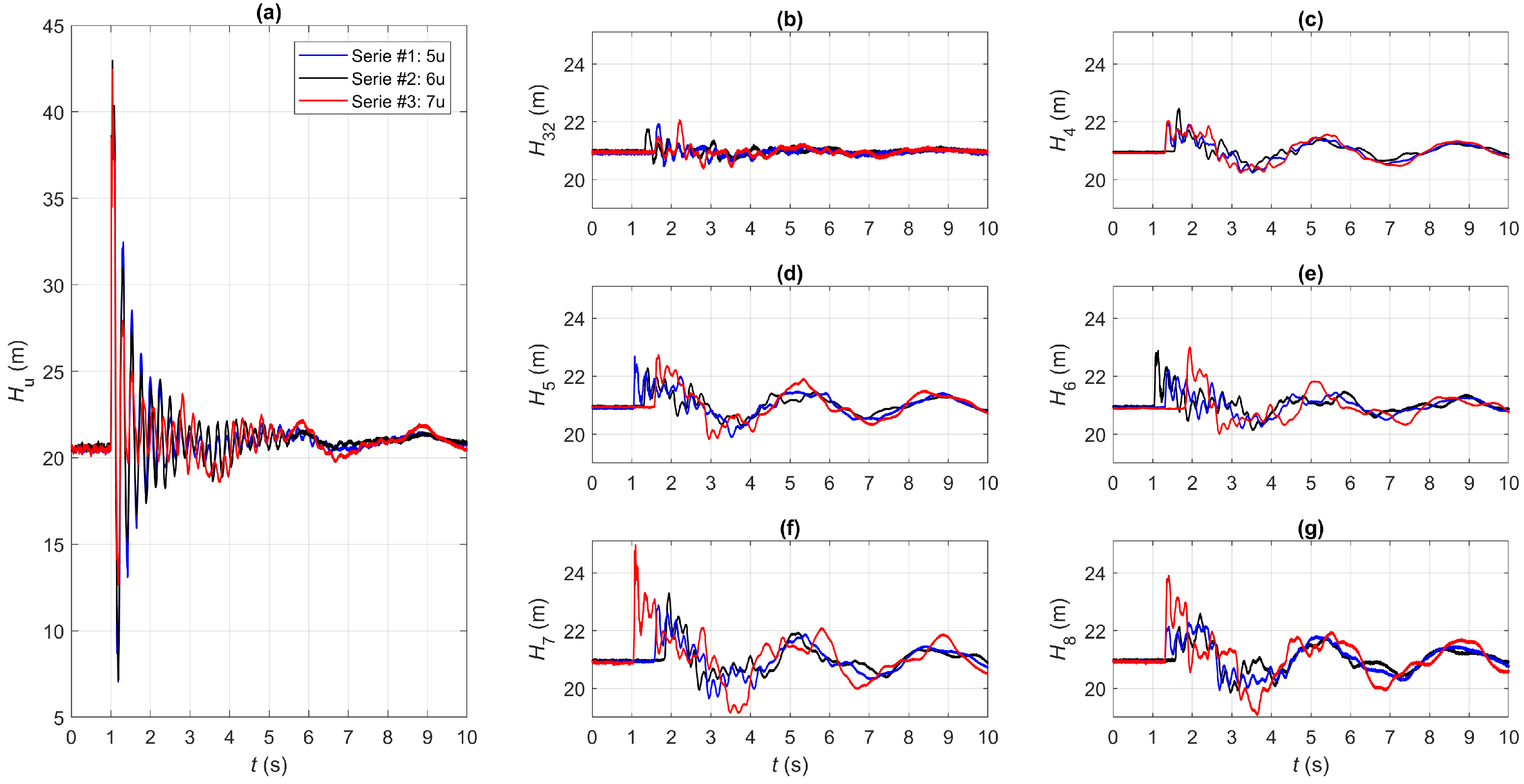
Figure 3 shows the pressure signals, H, acquired during test #1; in this figure, t = 0 indicates the manoeuvre starting time. Figure 3a highlights that at 5u the pressure variation due to the maneuver becomes trapped into the branch. Thus, the service line is overexcited since most of the incident pressure wave is reflected back by junction 5, whereas very small pressure waves propagate into the network.

Figure 3b reports the pressure signals acquired at the measurement sections in the proximity of junction 5: nodes 5, 5${}_4$, 5${}_6$, and 5${}_8$ of Figure 1b. According to [32], because of the overlapping of the incident and reflected pressure waves, these signals are almost indistinguishable; their extreme values are smaller than the ones measured at the end-user 5u (Figure 3a). Such a feature reflects the fact that node 5, located at the upstream-end of the service line, experiences the same pressure variations occurring at 5u only for an extremely short time interval—and, then, not acquirable—because of the proximity of the junction.

Successively, the transmitted pressure waves arrive at the closest nodes 4, 6, and 8. The pressure signals of Figure 3c point out that the pressure variation at node 4 is slightly smaller than the ones at nodes 6 and 8, whereas the damping of the pressure peaks is quite similar at nodes 4 and 6, but smaller at node 8.

The pressure signals at the measurement sections 7 and 32 and at the upstream tank (node 1) are reported in Figure 3d. The first pressure wave arriving at node 7 is significantly larger than all the other ones, whereas node 32 is the least stressed one because of its proximity to the tank.

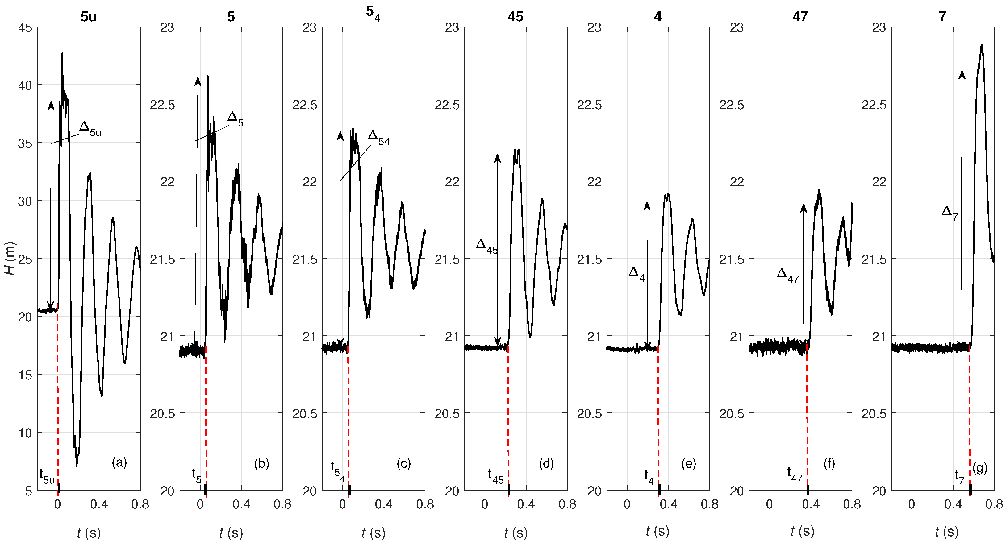
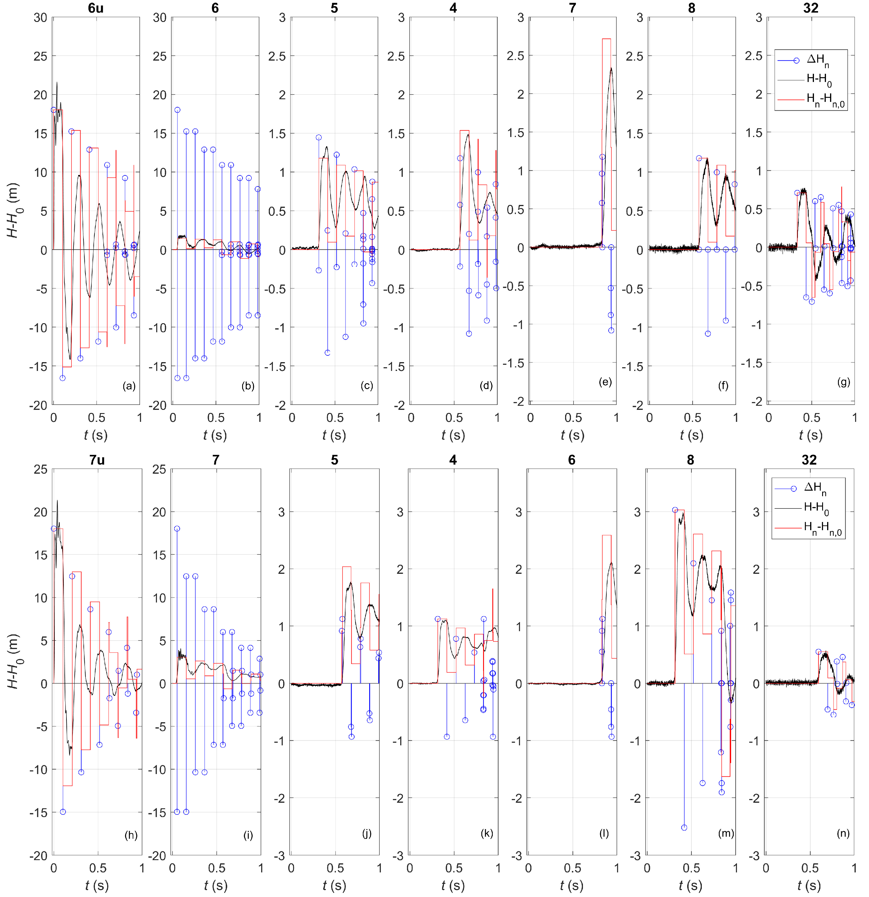
Figure 4 shows one of the paths travelled by the pressure wave generated at end-user 5u: at 5u (Figure 4a); at junction 5, connecting the service line to the network (Figure 4b); at the two measurement sections along the pipe connecting this junction to node 4: $5_4$ (Figure 4c)—1 m from junction 5—and 45 (Figure 4d)—69.3 m from junction 5; at junction 4 (Figure 4e); at the measurement section 47—28.5 m from junction 4 (Figure 4f); and finally at connection 7 (Figure 4g).

In this figure, the pressure variations due to the maneuver, ${\Delta }_m$, are also highlighted, with the subscript m indicating the measurement section. In Figure 4a, ${\Delta }_{5u}$ (=18.01 m) occurs at t = $t_{5u}$ = 0. At junction 5, ${\Delta }_{5u}$ is reduced by about 90 % because of the already mentioned interaction at this junction, resulting in quite a small pressure variation at $t_5$ = 0.05 s (${\Delta }_5$ = 1.78 m in Figure 4b) and $t_{5_4}$ = 0.053 s (${\Delta }_{5_4}$ = 1.42 m in Figure 4c). Successively, this pressure wave arrives at node 45 at $t_{45}$ = 0.219 s, with ${\Delta }_{45}$ = 1.28 m (Figure 4d). Then, at $t_4$ = 0.307 s, ${\Delta }_{45}$ interacts with junction 4, causing a smaller pressure variation (${\Delta }_4$ = 0.99 m in Figure 4e). In fact, part of the pressure wave is reflected back toward junction 5, and part is transmitted toward nodes 7 and 3. The transmitted pressure wave arrives at nodes 47 and 7 at $t_{47}$ = 0.384 s (Figure 4f), and $t_7$ = 0.577 s (Figure 4g), respectively. 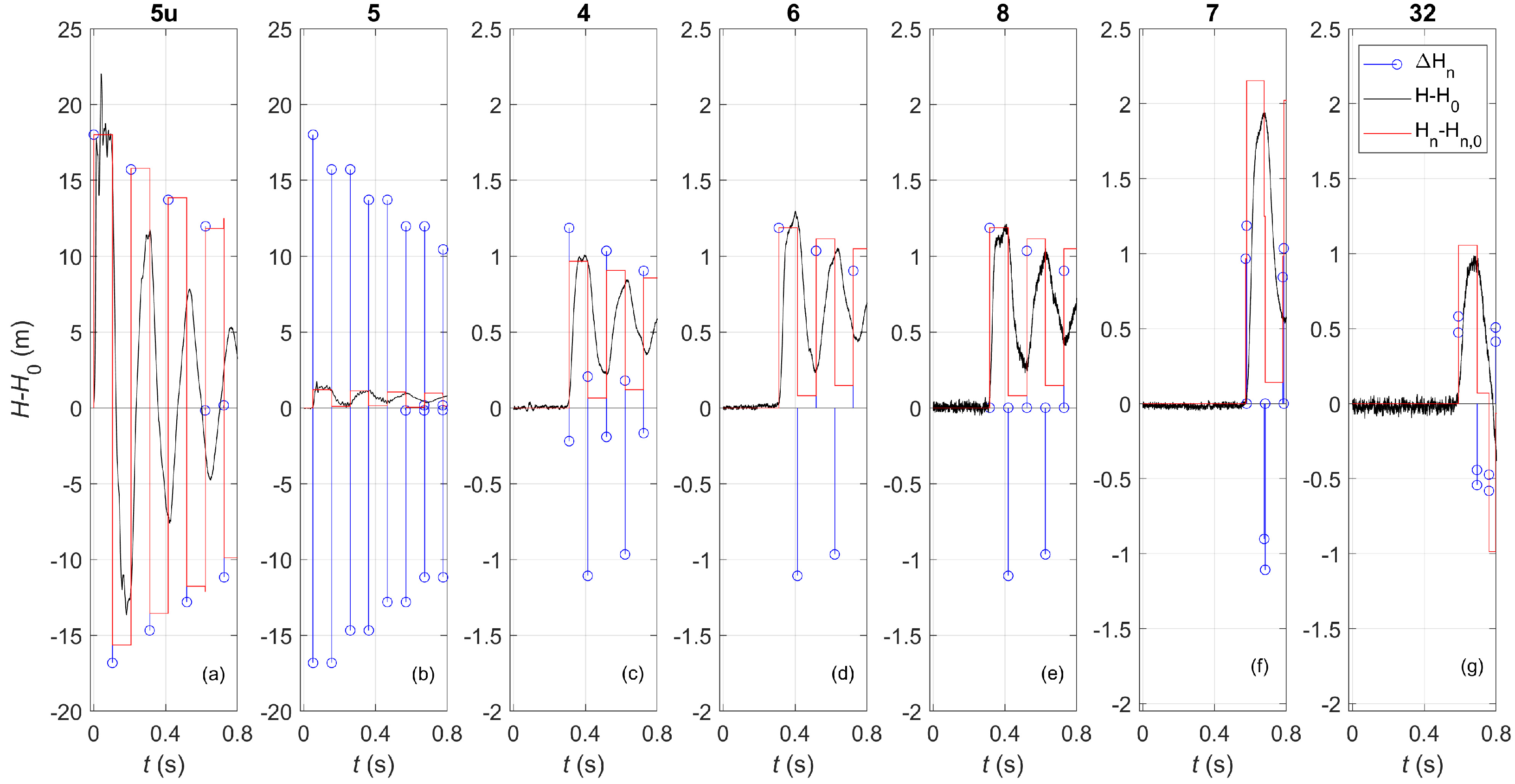Moreover, the amplitude of the transmitted pressure wave ${\Delta }_{47}$ (=0.92 m) is unexpectedly amplified at node 7 (${\Delta }_7$ = 1.75 m). Such a rise cannot be ascribed to the geometrical and mechanical characteristics of node 7 that is a connection in series between two DN50 equivalent pipes. On the contrary, it can be associated to the almost simultaneous arrival of different pressure waves, as it will be clarified below. To better explain such a behavior, the LM is used. In Figure 5, the results of the LM are compared to the experimental pressure disturbances, $H-H_0$, at some of the measurement sections (black lines). The blue stems represent the pressure waves given by the LM (i.e., the impulse response function), $\Delta H_n$, whereas the red lines depict the LM simulation, $H_n-H_{n,0}$. Figure 5b shows that the excitation at junction 5 is almost twice as the one at the end-user 5u (Figure 5a). In fact, the reflection coefficient at junction 5, $C_{R,5}$, is equal to -0.93, for a pressure wave arriving from 5u. In other words, the incident pressure wave is always followed by a reflected one with approximately the same amplitude but opposite sign. The transmitted pressure wave at junction 5 reaches the closest sections (junction 4 and connections 6 and 8). However, while these pressure waves cross undisturbed connections 6 (Figure 5d) and 8 (Figure 5e), with $\Delta H_{n,8}$ = $\Delta H_{n,6}$ = 1.19 m, junction 4 (Figure 5c) causes a reflection and a smaller resulting pressure variation ($H_{n,4}-H_{n,4,0}$ = 0.97 m). In addition, the first experimental pressure variation at node 8, ${\Delta }_8$ (=1.13 m), is smaller than the one at node 6, ${\Delta }_6$ (= 1.17 m), because of the larger friction losses along a DN50 pipe with respect to a DN75 one. Moreover, at connection 7 the close arrival of the two pressure waves transmitted at junction 4 and 8 causes the mentioned large pressure variation (Figure 5f). Finally, because of the interaction with junction 3, the simultaneous arrival of the pressure waves from connection 6 and junction 4 at the measurement section 32 (Figure 5g) causes a smaller global pressure variation ($H_{n,32}-H_{n,32,0}$ = 1.06 m).

4. The Effect of the Transient Generation Point

In order to point out the effect of the transient generation point on the dynamic behavior of the network, transients generated by the closure of the end-users at 6u (test #2) and 7u (test #3) are compared with test #1. In particular, Figure 6 compares the pressure signals acquired at the main nodes among those of Figure 3 with the ones of tests #2 and #3 for a given steady-state discharge ($Q_{0,5u}$ = $Q_{0,6u}$ = $Q_{0,7u}$ = 0.12 L/s). Specifically, Figure 6a highlights that, even if the maneuver is the same, during the first phases of the transient, the service line is more excited when the maneuver is executed at the end-user 5u. In fact, as confirmed by the LM results (Figure 5 and Figure 7), $C_R$ at the junction that connects the service line to the network is larger in absolute terms in the case of a cross junction (as node 5 with $C_{R,5}=-0.93$ ) than a Y junction (as node 6, with $C_{R,6}$ = - 0.92 and node 7, with $C_{R,7}=-0.83$). The value of $C_{R,7}$ is smaller than the one of $C_{R,6}$, because of the smaller diameters of the pipes connected to the junction. Thus, this means that for test #3, larger pressure waves are transmitted from node 7 towards the network (Figure 6f vs. Figure 6d,e). Moreover, the LM confirms that in the first phases of all the considered tests the most stressed part of the network is that with the smallest diameter pipes: nodes 7 and 8 (Figure 6f,g).

5. Maps of Vulnerability by the Lagrangian Model (LM)

The extreme values of the pressure variations are reached in the first phases of the transients. As shown, in such a period, the LM can be considered a good compromise between the computational efforts (quite limited) and its reliability. Accordingly, it allows pinpointing the most excited part of the network in the first period. The substantial limitation of the LM—i.e., the fact that it does not simulate the damping of the pressure waves—does not appear decisive. In fact, with respect to transmission mains in a WDN, it makes less sense to assume that the boundary conditions and related flow condition last for a long period of time. 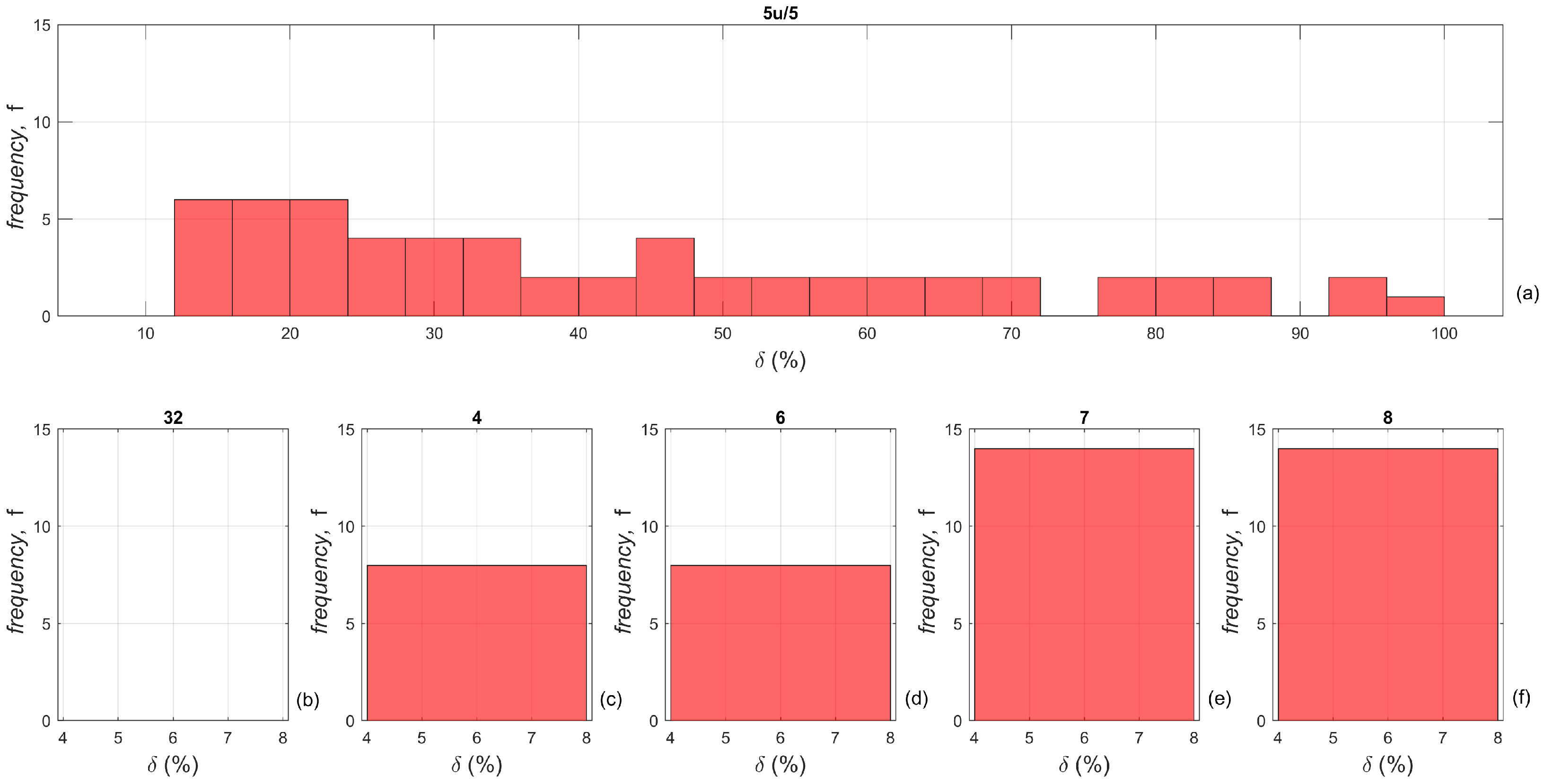In fact, as demonstrated in [38], because of the users’ behavior, flow conditions change so frequently that a stochastic approach is needed. In this context, the frequency distribution, f, of the numerical relative amplitude of the pressure waves, $\delta$, defined as:

$$\delta =\frac{|\Delta H_{n,m}|}{\Delta H_{AJ}}$$

(6)

has been evaluated for all measurement sections m, by considering pressure variations $\delta$, larger than a given value, ${\delta }^{*}$; in Equation (6) $\Delta H_{AJ}$ is the Allievi–Joukowsky overpressure. Figure 8—where it has been assumed, as an example, ${\delta }^{*}=4\%$—shows the frequency distribution, with a uniform width of 4 %, of the histogram bins. In particular, the largest values of $\delta$ occur for the service line: the start node (5) and end node (5u) behave equivalently, with $\delta$ being 10 times larger than all the other sections in the network. This confirms the results of the laboratory tests. However, the frequency of these large pressure variations is quite limited, with f = 2 for $\delta \ge 50\%$. To emphasize the behavior of the network nodes, a magnified vision of the frequency distribution for $4\%\le \delta \le 8\%$ is reported in Figure 8b–f. As already pointed out, the network is less excited than the service line. Moreover, the smaller the diameter, the larger the frequency: the maximum value of f (=15) is achieved at nodes 7 and 8, whereas it is f = 0 at node 32. This frequency distribution is used to synthesize the transient response of the system: both the frequency of occurrence of a specific $\delta$, and the amplitude of $\delta$ are taken into account in the vulnerability index, $\nu$, defined as:

$$\nu =\sum _i{f}_i{\delta }_i$$

(7)

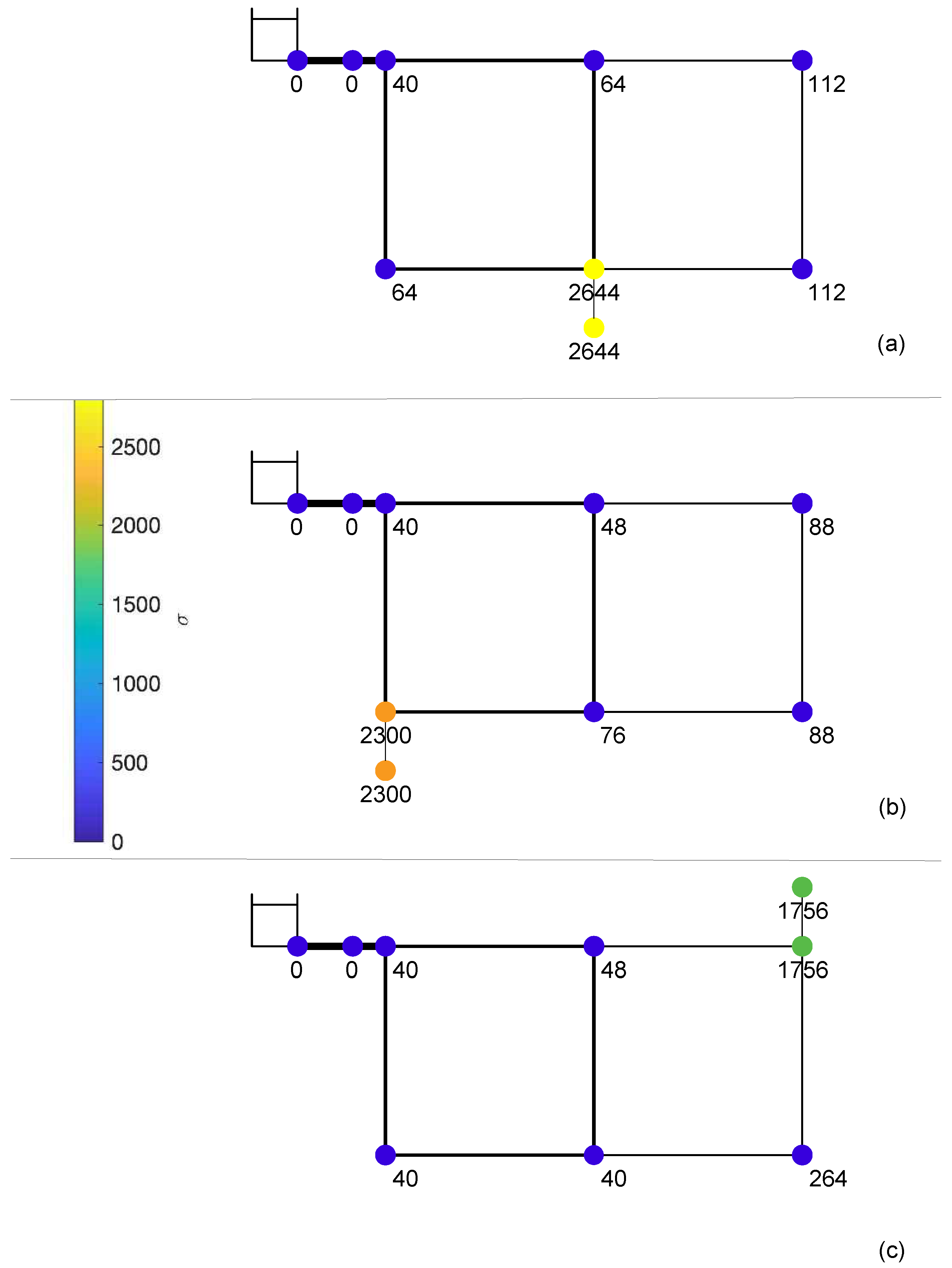
For all nodes of the network, the map of vulnerability is provided for the configurations of tests # 1, 2, and 3 (Figure 9), based on the values of $\nu$. The aim of these maps is to quickly identify the areas where the impact of transients is expected to be the largest and that may therefore require particular attention, in terms, as an example, of high-frequency pressure monitoring. As expected, according to the experiments, in all configurations the most stressed area is the service line. Moreover, the more complex the junction and the larger the diameter of pipes connected to the junction, the larger $\nu$. Finally, for all the tests, the most excited portion of the main network is the one with smaller diameter pipes (i.e., nodes 7 and 8), regardless of where the transient is generated.

6. Conclusions

In recent years, the idea that the effect of transients in water distribution networks is not negligible is gaining ground in the management of such systems. This is due to two main reasons. The first one is the more and more frequent occurrence of not negligible transients, due to the unavoidable users’ consumption variations and daily pump or automatic valve operation for system management. All these events, difficult to suppress or prevent by the water utilities, can lead to the deterioration of the system safety and long-term life cycles. In fact, the conventional surge protection devices (e.g., air vessel) are usually installed in the main pipes. The second reason is the fact that the steady-state modelling and low-frequency monitoring (i.e., of the order of 10${}^{-3}$ Hz) do not allow identifying the causes of leakage and faults occurring in only some parts of the network substantially equal to other ones in terms of pipe material, maintenance, and pressure regime. A possible explanation of such a feature could derive from an inappropriate identification of the nature of the actually dangerous transients and the different exposure to pressure waves of the different parts of the considered network.

This paper experimentally analyses the effects of a transient simulating an end-user closure in a looped water distribution network. The end-user located at the downstream end section of a quite long service line allows capturing each single pressure wave inserted into the network. The experimental tests and the successive analysis by means of a Lagrangian model highlights the effect of the network topology and the location of the transient generation point, but in a more expeditious way with respect to the use of a complete transient model. The assumption of the Lagrangian model of neglecting the friction terms and maneuver duration does not limit its use for interpreting the dynamic response of the system in the first phases of the transients.

In particular, the tests point out that the most excited part of the system is the one in close proximity of the end-user and then the corresponding service line. In fact, the generated pressure wave becomes trapped in the service line because of the severe reflection from the junction that connects the service line to the network.

In addition, when different pipe materials are considered, the general results could be considered analogous (not shown for the sake of brevity). In fact, even if the metallic pipes have a stronger compressive capacity than the plastic ones, a pressure variation in a metallic pipe generated by a given water consumption change is much larger (about double) than the one generated in a plastic pipe with the same diameter.

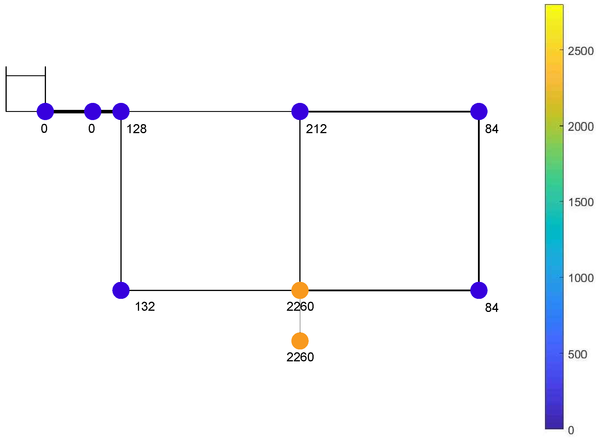
Furthermore, notwithstanding the transient generation point, the pressure waves entering into the network are 80–90% smaller than the generated one and accumulate in the parts of the network with the smallest diameter pipes. To demonstrate that the obtained results are not dependent on the chosen layout, the distribution of DN50 and DN75 pipes has been changed and reversed, and the indexes of vulnerability have been evaluated. As an example, Figure 10 shows the map of vulnerability, when the maneuver has been executed at node 5u. The results confirm that the service line is overexcited, and the smaller the diameter, the larger the pipe vulnerability, with the larger values of $\nu$ occurring at nodes 3, 4, and 6 that are in this case the junctions connecting the smallest diameter pipes.

It is worth pointing out that not the entity but the frequency of such waves could be potentially risky for infrastructure safety through fatigue loading. In other words, the regular occurrence of pressure transients (even if small) could contribute to the degradation of pipe materials, pipeline accessories, pipe support, and instrument failures (e.g., [37]).

In conclusion, by means of the Lagrangian model, which has been verified to be able to capture the pressure extreme values occurring in the first phases of the transient, the vulnerability maps of network are provided. These maps identify the nodes subjected to the most severe pressure waves in terms of both frequency and amplitude. The level of exposure to transients of each node is synthesized by the value of the vulnerability index proposed in this paper. Such an outcome could be of paramount importance for system maintenance and management and to address appropriate guidelines for fault prevention.