1. Introduction
The assessment of groundwater circulation in natural media, which are complex and irregular systems, needs specific hydraulic, hydrogeological and geometric assumptions and simplifications; this assessment can be carried out by resorting to aquifer modelling techniques, based on the use of different geo-informatics tools that allow for the proposition of possible scenarios of groundwater flow.
The investigation of karst aquifers is not easy to carry out due to the complexity and heterogeneity of such natural systems, where groundwater circulation occurs through a well-structured net of cave and conduits [
1]. The groundwater modelling in karst aquifers in southern Italy relies on some assumptions which represent the benchmark for the design of the conceptual model. In particular, the methodology followed using the MODFLOW numerical code implementation relies on the Darcy law and laminar conditions of the flow expressed by the Reynolds number, only applicable to the matrix domain of the aquifer. As the karst system is characterized by extreme types of porosity, connected to the presence of voids of different sizes, from the matrix to the conduit/cave systems [
2], the Darcy law can be applied to the flow system into the matrix portion, whereas it becomes hardly achievable in aquifers that are strongly fractured and affected by a highly developed net of conduits/shafts, which need different approaches. Among different numerical codes, the tool which better simulates the groundwater flow for the saturated zone, at a regional and subregional scale [
3], is the MODFLOW numerical code [
4,
5,
6], which allows one to assess the flow path, calibrating the simulated hydraulic parameters on the observed data.
Several authors focused on groundwater flow modelling to simulate the aquifer behavior and provide forecast scenarios, through different mathematical and statistical approaches [
7,
8,
9]. However, groundwater models are affected by an uncertainty degree, because they represent a simplification of natural and complex hydrogeological systems. Teutsch [
10] proposed a model to simulate the flow within an aquifer that was moderately karstified, for a catchment area of the Swabian Alb, considering a porous-equivalent medium (EPM model).
For Barton springs (Texas), which belong to a high karstified aquifer, a regional groundwater model has been proposed by Scanlon et al. [
11]. Huntoon [
12] highlights that the EPM hydraulic approach is suitable if we analyze the regional groundwater flow but that it is not taken into account to examine the hydraulic and hydrogeological aspects at the local scale and near the spring zone. Halihan and Wicks [
13] focused on the effect of the karst/shaft conduit net on the karst aquifer response, proposing a discrete fracture model (DF), assuming that the flow occurs mainly in the conduit net and that no water exchange between the shaft net and aquifer matrix occurs.
Panagopoulos [
14] simulated the groundwater flow in the Trifilia karst aquifer, Greece, providing different scenarios and using MODFLOW both in the steady state and for transient conditions. Hill [
8] proposed a simplified approach for groundwater modelling because all models in natural systems are simplifications; then, the number of parameters considered to build the model is the primary measure of its simplicity or complexity.
Several groundwater models refer to regional groundwater flow [
15], which better depicts the groundwater flow from the recharge area to the discharge zone, describing further the flow pattern in a hierarchically nested composite basin. The groundwater flow theory was widely proposed by Toth [
15] and other hydrogeologists and karst hydrogeologists; the theory was physically and mathematically demonstrated. Successively, the theory was applied considering specific tools which allow for the automation of the groundwater flow conceptual model. Just as for other tools [
16], the MODFLOW numerical code that was used to characterize groundwater flow also allowed for the further enrichment of knowledge on groundwater behavior through the design of a specific model in which the calibration phase assumes a crucial role because it is preparatory for the following steps of aquifer modelling.
Karst aquifers are mainly characterized by a dual system due to the presence of different flowpaths, including (i) a quick flow in karst conduits and channels, and (ii) a slow flow in the matrix and micro fracture network [
17]; then, the use of the CFP (Conduit Flow Process) package is strongly recommended for highly karstified aquifers.
However, some karst systems behave as porous-media that is hydraulically homogeneous, which allows one to apply the physical and hydraulic basics of the Darcy law, considering laminar flow conditions. In particular, the Caposele aquifer highlights a behavior that is more similar to the porous-equivalent medium [
18] than to the karst medium, allowing for the simulation of the aquifer, assuming specific conditions for the hydraulic model. In this study, a hydraulic model was built using the MODFLOW numerical code for a generic aquifer that was completely drained by a unique spring outlet, after which the simulation was also extended to the Caposele aquifer (southern Italy), where different flow simulation tools were used, taking into account the hydraulic and hydrogeological features of the spring catchment.
The model that was designed allowed for the estimation of the Darcian travel time of groundwater into the saturated zone and the geometry of the groundwater flow path, using the MODPATH package, providing different scenarios of the groundwater level. In particular, the role of the thickness of the aquifer’ saturated zone on the flow net distribution was discussed; a general ascendant flow feeding the spring was also inferred in analyzing a cross-section near the discharge area.
2. Materials and Methods
The groundwater flow was simulated for an unconfined aquifer in a steady-state condition, focusing on the saturated aquifer zone according to the Darcy law [
19], through which the filtration velocity,
v, can be expressed by Equation (1):
where
K is the hydraulic conductivity of the medium, and
i is the hydraulic gradient, expressed as the ratio between the hydraulic head difference,
, and the spatial coordinate of the filtration direction,
. As the Darcian velocity is generally not available but can be estimated, the aim of mathematical-physical models is properly to assess the hydraulic head for different scenarios and stress conditions. Considering an incompressible fluid, combining the mass conservation law with the Darcy equation, a partial derivative equation was obtained, describing the flow yield of groundwater in a steady state condition [
20,
21]:
By using Equation (2), the water extracted for the volume unit from the porous medium (
W) based on the coordinate of the filtration direction,
, can be estimated, considering the principal component of the hydraulic conductivity tensors
Kxx,
Kyy and
Kzz, aligned with the x-, y-, and z-axes [
22].
The hydraulic approach developed in order to analyze and model groundwater was described for a generic aquifer totally drained by a unique spring outlet, and was then applied to the Caposele spring catchment. The general model can be considered a benchmark that is then applicable to aquifers with the same hydraulic and hydrogeological properties as for the study area.
The MODFLOW numerical code was used, simulating groundwater flow in the saturated zone of the aquifer, based on the conceptual model designed for the study area [
4]; then, the code was implemented through the graphic user interface PROCESSING MODFLOW 5.3, which simplified the calculation code. The MODPATH package [
23] allows one to calculate the particle paths and travel times of the particle trajectory in order to define the flow net, using a semi-analytical algorithm to draw the water particle.
Figure 1 highlights a plan view (horizontal) of the groundwater model of a generic aquifer (obtained by 3D flow simulation) drained by a unique spring outlet and characterized by a regular shape. The groundwater modelling was carried out simplifying the groundwater framework [
24], where physical and hydraulic parameters were mathematically integrated on the vertical plane, as equipotential lines, [
25,
26,
27,
28,
29].
Figure 1 shows the flow net obtained for an unconfined aquifer, square shape with a 7500 m length of side, grid characterized by 22.500 cells, and with a dimension of 50 × 50 m; vertically, the model discretization was carried out for a maximum model depth of 2000 m considering two equally sized layers. In accordance with the MODFLOW simulation, a regular flow net was drawn, in which the flow lines converge towards a unique spring outlet.
Assigning specific boundary conditions to the model, the hydraulic head of the spring was considered constant during the flow simulation (Dirichlet type condition), and the recharge amount was modulated on the spring discharge (Neumann type condition).
In this model, the hydraulic head progressively decreases towards spring; conversely, the slope of the water table progressively increases towards spring. Even if the flow net shape depends on the geometry of the aquifer, the recharge amount and the hydraulic conductivity of the medium rule the maximum hydraulic head in the aquifer, following which the hydraulic head value drops between two consecutive equipotential lines.
Based on the grid shown in
Figure 1, the model domain was also analyzed considering cross sections drawn along the entire spring catchment area to highlight the groundwater flow in depth. To analyze the flow in depth, and go over the
Dupuit-Forchheimer conditions used to build the plan model, a 2D analysis was carried out along a vertical plane. In this case, the boundary conditions fixed to build the general model were taken from the result obtained by the horizontal model.
In particular, the hydraulic head values along the cross-sections of
Figure 1 (AS, BS and CS) were imposed into the 2D vertical model to find the geometry of the flow net in depth.
Figure 2 shows the results of the modelling along the vertical cross sections AS, BS and CS, where each different flow pipe is distinguished by different colors, for a total of n.7 flow pipes in this example. The flow net in the vertical plane was obtained using MODPATH package. Of course, the geometry of the flow net and the number of flow pipes depend on the thickness of the aquifer’s saturated zone (TSZ), which plays a crucial role in flow paths, as the more thickly saturated zone implies the higher the travel time. The model was also run for different values of the effective porosity n
eff considering the range 0.01–0.10 [
30]; even if the effective porosity ruled the flow net geometry, in particular the groundwater travel time, no significant differences were found for the considered n
eff range, representative of these kinds of aquifers; as described in the following sections, the hydraulic conductivity, K, has an important role in controlling the flow net shape.
Even if this procedure could be an approximation of a more complex 3D model, it could provide a useful simplification of the flow net geometry both horizontally and vertically, allowing for the further considerations that are described below.
Considering the common flow pipe of different cross-sections (
Figure 2), in a plan-view it is possible to extrapolate the origin of flow pipes by interpolation, considering the beginning of the flow line boundaries of each flow pipe.
Figure 3 provides a plan-view of the starting path of each flow pipe, which corresponds to zones 1 to 7; this representation has been obtained through a combined use of the GIS-MODFLOW tools, interpolating the flow pipe boundaries on the horizontal plane.
In
Figure 3, the different zones (from 1 to 7) contribute differently to aquifer discharge: the most distant ones from the spring are also wider, and they are characterized by a deeper flux, whereas the closest to the hydraulic outlet are smaller and are affected by a shallower flux.
The simple zonation of the aquifer shown in
Figure 3, considering an isotropic and homogenous aquifer, allowing one to investigate the contribution of different hydraulic sectors to the spring, in terms of the percentage of total discharge and the time that the flow needs to reach the final outlet. In particular, the catchment area zoning in different flow pipes allows one to estimate the different recharge volumes and different contributions to spring discharge (Equation (3)). The contribution to the discharge
Qi of each flow pipe can expressed by:
where
R is the recharge amount, expressed as a length/time, [L/t], imposed as constant on the entire catchment (
Neumann condition), and
FPAi is a generic flow pipe area. Applying Equation (4), the total amount of the discharge
QS is computed:
where
n is the number of flow pipes. To estimate the travel time along each flow line, and to evaluate the (Darcian) mean travel time to reach the spring, Equations (5) and (6) were applied, considering steady state conditions and the Darcy regime (laminar flow). The time,
tλ, needed between two equipotential lines with length
Lλ is:
and the total time,
ti, estimated along the entire flow line,
i, is:
where
m is the number of equipotential lines along the flow line
i. The total time
ti of the flow line
i can be assumed constant for a generic flow pipe
i, and each flow pipe area of
Figure 3 would be characterized by a specific travel time to reach the spring. This simplification allows one to provide the following considerations about the (Darcian) mean travel time of the spring water,
tS, which can estimated by:
The actual travel time, t’
S, can be found knowing the effective porosity of the medium, n
eff:
The aquifer zoning in flow pipe areas also allows one to estimate the age of the groundwater (Equations (7) and (8)), following which we can assess the older and younger zones of groundwater circulation in the saturated zone of the spring catchment area. The flow pipes assessment leads to zoning the aquifer in different hydraulic sectors, which behave differently in recharge-discharge processes; this approach also allows one to estimate the contribution to spring discharge of each sector, getting a preliminary estimation of groundwater velocity in shallow and deep zones of the aquifer. Particularly, a travel time assessment in aquifers, with the estimation of the groundwater age, is a crucial hydraulic aspect for the modeler; the knowledge of the groundwater age, with its relative hydraulic and physical parameters, allows one to understand several hydrogeological and hydrogeochemical phenomena connected to intrinsic groundwater vulnerability [
31] and the specific vulnerability of water bodies to contamination [
32,
33].
2.1. Geological and Hydrogeological Features
The Caposele spring is fed by the northern sector of the Picentini Mountains (
Figure 4), where the Cervialto massif is the highest mountain (1809 m a.s.l.). This area is characterized by high slope angles, connected to Quaternary tectonic uplift, which has caused several fault-scarps in the carbonaceous rocks, actually showing a slope angle around 35°–45°. Locally, a series of limestone and limestone-dolomite (Late Triassic-Miocene) outcrops, characterized by a thickness ranging between 2500 m and 3000 m, are generally extremely faulted and crushed. Along the northern and eastern sectors, these massifs overlap tectonically on the terrigenous and impermeable deposits (
Figure 4), constituting argillaceous complexes (Paleocene) and flysch sequences (Miocene).
A more specific geological insight on the outcropping areas can be found in Vitale and Ciarcia [
34] and related literature, and in the Geological Map of Italy, 1:50.000 scale (Foglio 450, Sant’Angelo dei Lombardi; Foglio 468, Eboli) provided by Istituto Superiore per la Protezione e la Ricerca Ambientale, ISPRA [
35]. Pyroclastic deposits of the Somma-Vesuvius activity cover the Picentini Mountains, with thicknesses of up to several meters along gentle slopes and only a few decimeters along steep slopes.
The pyroclastic cover is generally composed of several irregular, ashy pumiceous layers, intercalated with weathered ash deposits. All these deposits have high water retention values and play an important role in the infiltration of water into the karst substratum. Wide endorheic areas (
Figure 4) characterize these mountains, having also an important role in the recharge processes [
36,
37,
38]. The origin of these endorheic zones is connected to tectonic activity during upper Pliocene-Pleistocene, which has triggered a general uplift by normal faults and the formation of graben zones. During the following continental environment (Pleistocene-Holocene), karst processes transformed these zones into endorheic ones, allowing the complete absorption of runoff and the formation of seasonal lakes. The largest is the Piano Laceno (20.5 km
2), where a small sinking lake exists, which increases during the winter-spring period. As the Caposele spring can be considered the only spring draining the Cervialto Massif (other springs have a considerably lower discharge), this entire endorheic area constitutes part of the recharge area of this spring. Considering the hydrogeological and morphological features, the total estimated recharge area is 110 km
2 [
36], which practically feeds only the Caposele spring.
The Caposele aquifer appears as a slight or moderate karstified system, and the spring discharge is characterized by the smooth shape of the hydrograph, with the absence of a quick flow component [
18]. During the hydrological year, two main periods can be distinguished: the high-flow period during spring-summer time, and the low-flow period during the autumn-winter time; in a typical Mediterranean climate, this characteristic of the flow causes a quasi-opposite response to the rainfall distribution.
Figure 5 shows the Caposele daily spring discharge in the period March 2012–March 2019, with a mean value of 3690 l/s. The minimum occurred in winter 2017, after a long dry period; the maximum occurred in summer 2013, after a very wet hydrological year.
Figure 5 also shows the water table level detected in a borehole, P1, located about 400 m from the spring (
Figure 4); as the water level into P1 was well-correlated with the spring discharge, it was used for model calibration.
The trend inferred by the spring hydrograph analysis highlights the smooth discharge fluctuation, proving the hydraulic behavior of the investigated aquifer; this appears similar to a porous-equivalent medium, thus justifying the use of the EPM approach.
2.2. Conceptual and Numerical Model of Caposele Aquifer
The aim pursued by the modeler in a numerical groundwater simulation is to provide a useful tool supporting the planning and the management of water resources, safeguarding them both quantitatively and qualitatively.
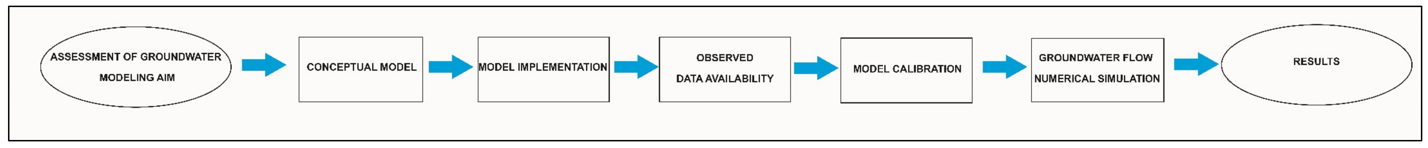
The implementation of a flow mathematical model requires the assessment of a conceptual model for the investigated area. The workflow of
Figure 6 summarizes all steps carried out for a groundwater numerical simulation. The conceptual model assessment, in accordance with the geological and hydrogeological features of the Caposele groundwater catchment (
Figure 4), plays a fundamental role in the scenarios proposed by the groundwater flow simulation, representing a preparatory phase for the implementation of a numerical model. The shapefile of the Caposele spring catchment was edited using the GIS environment, and was then imported to identify the model domain. The boundaries of the catchment area are coherent with the geological and hydrogeological features of the investigated area, characterized by a karst aquifer with a high transmissivity bounded by a flysch sequence along the northern side and a less permeable dolomite sequence on the southern side; then, the structured grid was defined.
As the aquifer depth was unknown, the model was run for different thicknesses of the aquifer’s saturated zone (TSZ) (100 m, 200 m, 500 m, 1000 m and 2000 m) in order to consider a wide thickness range. The Caposele model domain was defined considering a square with a side of 15 km; then, the grid of the study area was arranged in a plan with a cell sized 100 m × 100 m, providing a grid with 22500 cells. Along the vertical direction, the model was built considering two layers with equal thicknesses and was run in a steady state condition considering an unconfined aquifer. The boundary conditions were defined according to the physical, hydraulic and hydrogeological features of the modeled area [
39].
Among several methodologies to characterize spring cells, the use of a first type condition of Dirichlet appears to be the best approach for simulating groundwater flow in a natural system such as the investigated aquifer, which is not influenced by artificial drainage.
The initial and boundary conditions were established considering the discharge value of the spring in order to attribute a recharge amount to the domain (Neumann type condition); then, the hydraulic conductivity, K, was assigned and calibrated considering the water table level of the P1 borehole. A constant hydraulic head (417 m a.s.l.) was considered for the cell of the Caposele spring (Dirichlet type condition).
The annual mean water amount recharging the aquifer, R, was expressed as the recharge height, estimated by the ratio between the Caposele spring discharged volume and the catchment area, AC, providing (R)AC = 1.06 m/y.
Figure 7 highlights the attribution of the recharge to the model domain considering the graphic user interface VISUAL MODFLOW FLEX 2015.1; in the first case (
Figure 7a), we fixed a recharge uniformly distributed on the catchment area, while
Figure 7b, taking into account topographic features, shows the discretization of the recharge considering both endorheic and open areas.
We have considered the recharge amount for endorheic areas,
(R)AE, in which rainfall totally infiltrates (
Figure 7b), whereas a minor amount has been considered for open areas of catchment, (
R)
AO, on which the runoff is 34%, as estimated by Fiorillo et al. [
36]; of course, the overall mean recharge on the spring catchment remains (
R)AC = 1.06 m/y, with respect to the same amount discharged by the spring outlet.
As the recharge discretization between the closed and open areas of spring catchment does not lead to significant change during flow simulations, we mainly focused on the recharge uniformly distributed on the model domain in order to provide the simplest model.
Following the Neumann-type boundary condition with null flow along the borders of the catchment area, the grid inside the shapefile of the aquifer drained by the Caposele spring is active for groundwater modelling (flow zone), whereas outside no flow occurs (no flow zone).
As concerns the unsaturated zone, even if the vadose zone and its hydraulic features play a crucial role for the Caposele spring catchment, modulating the discharge response [
18,
40], the numerical code applied in this work (graphic user interface PROCESSING MODFLOW 5.3) mainly focused on the hydraulic behavior of the saturated zone of the aquifer under steady-state conditions. However, the thickness and hydraulic conditions of the unsaturated zone, and the connected percolation processes, become especially relevant for the transient flow condition; these aspects need further in-depth analysis, also using further tools such as MODFLOW SURFACT, R-UNSAT, VS2DI or FEFLOW.
2.3. Model Calibration
First of all, the boundary conditions and the recharge amount for a steady state model were fixed. Successively, the calibration of the model was carried out based on hydraulic head data available for the P1 borehole, varying the input parameter of the hydraulic conductivity until similar values were found for the simulated (output parameter) and observed P1 hydraulic heads.
According to some specific procedures, such as the
trial and error method and
automatic calibration techniques, the calibration phase represents the process through which the hydraulic parameters provided in the input for the model are modified, so that they are matched with the observed data. This can be considered a benchmark phase for groundwater modelling because it is preparatory for the implementation of the simulations having a predictive purpose [
22], also allowing one to provide for the lack of hydraulic and hydrogeological data. As some physical and hydraulic parameters are not available, the simulated hydraulic conductivity was calibrated on the hydraulic head data of the P1 borehole detected during the time period of March 2012–March 2019; this well is located within the catchment area, about 400 m upstream of the spring outlet.
Figure 8 shows different simulations of the model considering different thicknesses of the aquifer’s saturated zone (TSZ), taking into account the narrow values of the hydraulic conductivity,
K; in particular, using the constant recharge amount
R = 1.06 m/y, and considering the mean value of the hydraulic head detected in the borehole P1,
h = 422.16 m a.s.l., the
K value was found to range from a maximum of 0.01145 m/s, (TSZ = 100 m) to a minimum value of 0.000831 m/s ascribable to a TSZ = 2000 m. The calibration phase highlights the relationship occurring between the TSZ of the aquifer and the hydraulic conductivity of the medium for 3D groundwater, using the EPM approach.
In particular, the
trial and error method, used to match the simulated hydraulic head with the available observed data, highlights that the hydraulic conductivity of the medium drops with the increase of the aquifer TSZ, in accordance with the hydraulic assumptions followed to build the conceptual and numerical model (
Dirichlet and
Neumann conditions). The hydraulic conductivity range found for different scenarios is in agreement with the K values estimated for other karst systems in southern Italy [
41,
42].
3. Results
The preliminary phase for the groundwater simulation carried out for the investigated aquifer allowed us to get a possible scenario of the mean hydraulic head. It was deduced by model calibration, assuming the abovementioned conceptual model boundary conditions.
Figure 9 highlights the maximum and minimum groundwater levels for TSZ values of 100 m and 2000 m, respectively, considering the mean hydraulic conductivity K
mean = 0.0048 m/s obtained for all calibrations,
Figure 10 shows the Caposele aquifer fluctuation for different depths, considering a mean recharge amount (R = 1.06 m/y); then, the simulation was also carried out considering high recharge (2 × R) and low recharge periods (0.5 × R).
The simulation points out that the hydraulic head of the recharge area drops when TSZ increases, fixing the K
mean value as being constant for all the proposed scenarios (
Figure 10). This preliminary result allows one to obtain a relationship between the groundwater level fluctuation and aquifer depth, providing details on the water table slope. According to the proposed scenarios, thicker aquifers are characterized by a flat water table, while conversely, a high slope of the water table can be considered an indicator of a saturated zone with less thickness; this also allows one to claim that aquifers characterized by a flat water table are affected by deep groundwater circulation, whereas a higher water table slope is a marker of shallow flow paths.
The flow simulation provided hydraulic head arrays as the output parameters for the model, leading us to hypothesize a possible scenario of the Caposele unconfined aquifer’s hydraulic behavior under a steady state condition. Based on the conceptual model assumptions, the hydraulic head,
h, estimated by simulation, ranges between the lowest value at the spring (h
min = 417 m a.s.l.) and the mean of the maximum values reached in all simulations, h
max ≈ 427.5 m a.s.l. in the recharge area, estimated for the mean recharge condition. Considering the hydraulic head difference between the recharge area and the Caposele spring, Δh ≈ 10.5 m, the water table slope has a mean value of about 0.001, which is in agreement with the slope found for other karst aquifers of central-southern Italy [
30,
43]. However, due to its non-linearity, the slope of the water table progressively increases toward the spring [
43,
44]; in particular, it has a mean value of 0.008 between the P1 borehole and the spring, and it is almost flat when far from the spring.
The hydraulic head difference that was found, Δh ≈ 10.5 m, between the maximum recharge area and the Caposele spring, was proven considering the n.5 groundwater level scenarios proposed for different aquifer TSZs. However, the hydraulic head difference that was estimated is a mean value because it can fluctuate during the hydrological year, reaching values that are higher and lower than the mean value.
3.1. Assessment of Travel Time on Caposele Aquifer
The MODFLOW numerical code used to simulate the groundwater flow for the Caposele aquifer is able to compute the travel time of water along the groundwater flow net.
Particularly, the MODPATH package is able to calculate the groundwater paths together with the velocity vectors estimated cell-by-cell; the effective porosity value, n
eff, included in the range 0.01–0.10, was considered for the simulations [
30]; then, in order to obtain the travel time for each flow pipe, the MODPATH groundwater flow net was investigated according to the hydraulic approach described by Equations (3)–(7).
Table 1 shows the main results obtained by the Caposele aquifer modelling, considering different TSZs, up to a maximum thickness of 2000 m. As the actual effective porosity parameter is not available and no environmental tracers were used to evaluate the actual travel time (Equation (8)), the hydraulic approach adopted using the MODFLOW numerical code was able to find the Darcian (mean) travel time range for different scenarios.
The hydraulic conductivity of the medium was estimated by calibrating the model (
Figure 8), after which the Darcian velocity (Equation (1)) and Darcian travel time (Equations (5)–(7)) were also computed. Through a flow simulation, the estimated travel time, applying Equations (5)–(7), ranged from a minimum value of 45.8 years (TSZ = 100 m) to a maximum of 551.8 years (TSZ = 2000 m). Considering all scenarios, the hydraulic analysis highlights that the water particle flows faster considering the flow pipes near the spring zone, while, conversely, water needs more time to reach the spring outlet along the flow pipes that are more distant from the discharge area.
The hydraulic approach followed to estimate the travel time along the flow net of the Caposele aquifer using the MODFLOW numerical code also allows one to underline that the knowledge and the setting of the aquifer TSZ in groundwater modelling is crucial for the assessment of the hydraulic parameters of the aquifer.
The Darcian travel time trend, observed for the proposed scenarios, clearly points out fast groundwater paths for aquifers with less thickly saturated zones, and flow paths that are slower belonging to aquifers affected by thicker saturated zones.
In
Figure 11, the hydraulic conductivity and Darcian travel time were matched with different TSZs of the model. In particular, the hydraulic conductivity of the medium dropped when the model thickness increased, ranging from a maximum
K = 0.0115 m/s found for models with less thickly saturated zones to a minimum
K = 0.000831 m/s attributable to aquifers with a thickness of 2000 m.
The inverse relationship found between the K values and model thickness is coherent with 3D groundwater modelling. Considering the Caposele discharge as a fixed, unique and constant spring outlet, a thicker aquifer needs a low hydraulic conductivity and a long travel time to satisfy the same discharge of less thick model.
3.2. Flow Vectors
The flow pipes assessment for the investigated area allowed one to understand the hydraulic behavior of groundwater from the recharge zone toward the spring area. The numerical simulation of the Caposele aquifer also allowed one to estimate the flow vectors; in particular, the groundwater flow net highlighted the different flow directions along the aquifer (
Figure 12,
Table 2). The analysis focused on the area within 1 km upstream the Caposele spring, where the flow lines converge, following which the flow vectors were geometrically estimated.
Figure 12 shows the geometric approach followed to estimate the
x and
y vectors, whose values are duly tabulated. A hydraulic approach was proposed to assess the vertical and horizontal contributions of groundwater flow to spring discharge. Assuming that the medium can be considered homogeneous and hydraulically isotropic, and that the fluid is incompressible, the flow equation can be simplified under the
Laplace law [
45,
46]:
Here,
is a scalar function, twice differentiable in space; based on Equation (9) for the graphical solution of the 2D flow net, some hydraulic parameters of the Caposele groundwater flow were estimated. The simulation focused on the flow mesh of groundwater, on which the vectors analysis was performed. Then, the Darcian velocity was computed, considering the hydraulic conductivity obtained by model calibration and the relative hydraulic head (
Figure 8). To assess the vertical and horizontal contribution of groundwater flow to spring discharge, a geometrical approach was followed; its graphical results are described in
Figure 12.
For each flow mesh at a distance of up to about 1 km from the spring zone, the velocity vectors
vX and
vY and their relative discharges
QX and
QY were estimated. The main results obtained from the vector analysis are duly shown in
Table 2, pointing out the geometrical and analytical parameters obtained by the flow net analysis carried out along the 2D vertical plane of the Caposele spring zone. In particular, deeper flow meshes of groundwater highlight a predominance of the vertical velocity vectors
vY on
vX, and consequently the vertical component of the discharge
QY is predominant along deeper flow meshes. The ascendant flow detected near the spring zone is a hydraulic phenomenon common also to other springs of southern Italy [
41,
47].
3.3. Flow Pipes
The hydraulic approach and methodology argued for a generic model drained by a unique spring (
Figure 1,
Figure 2 and
Figure 3) was applied to the study area; accordingly, we carried out zoning on different flow pipes for the Caposele spring catchment.
In particular,
Figure 13a shows one of the cross-sections (B’S’) considered for the flow pipes assessment; the boundary conditions of the 2D vertical model were inferred by a 3D groundwater analysis on plan-view.
Figure 13b shows the map of the obtained flow pipes’ starting areas when running the model up to a maximum depth of 2000 m.
Considering the different scenarios proposed, the flow pipe areas farthest from the spring zone mainly contribute to spring discharge. Although their geometry varies with the aquifer TSZ, the preliminary results obtained in this paper support, for each scenario considered in the modelling, the major influence of flow pipe areas that are more distant from the spring zone in the discharge processes.
Given that for the flow pipe areas belonging to the maximum recharge area, water needs more time to reach the spring outlet, its relative travel time is higher than for flow pipe areas near the discharge zone; this means that, independently from the thickness chosen for the model, the groundwater age of the recharge area is higher than for the water flowing near the spring zone. The main hydraulic parameters of groundwater zoning in flow pipe areas for a model with a thickness of up to 2000 m are duly listed in
Table 3. In particular, the contribution to the discharge of different hydraulic sectors decreases towards the spring.
4. Discussion
Groundwater modelling was carried out for the Caposele karst aquifer, which has a hydraulic behavior similar to a porous-equivalent medium and an EPM approach was used. Nevertheless, a groundwater numerical simulation was also successfully applied to karstified aquifers [
10,
48,
49,
50], with satisfying results.
The input parameters in the flow simulation, together with an accurate modelling strategy [
51], play a crucial role for groundwater analysis, affecting the efficiency and then the interpretation of the model.
Emblanch et al. [
52] exploited chemical and isotopic tracers to evaluate the contribution of different water components discharging at the Fontaine de Vaucluse karst spring near Avignon (Southeastern France), considering two different hydrodynamic phenomena of the aquifers: (i) a perfect piston flow (PF), where each recharge event pushes the previous one towards the hydrological outlet; (ii) a well-mixed model (WMM), where the discharged water is a mixture between all aquifer components [
52,
53]; the aforementioned systems point out two extreme flow modalities; in nature in particular, the majority of aquifers highlight an intermediate behavior between the PF and WMM modalities.
The numerical simulation performed for the Caposele aquifer relies on the boundary conditions of the conceptual model subsequently implemented with the MODFLOW numerical code. The accuracy of the model depends on the number and kind of the assumptions, together with the type of mathematical and physical conditions on which it is based. A numerical flow simulation using the EPM approach is able to simplify the modelling of the heterogeneous structure as an aquifer system [
53,
54,
55,
56]. The methodology described in this paper, considering all workflow steps shown in
Figure 6, led to an understanding of the results obtained by both a travel time analysis and aquifer zoning in flow pipes, also allowing for the detection of a hydraulic phenomenon of ascendant flow near the discharge zone.
The groundwater flow simulation was carried out considering a combined 2D-3D approach because the model was run both along a cross-section (2D view) and a horizontal view (3D), considering a TSZ that was variable from 100 m up to 2000 m. The preliminary results obtained from the travel time assessment gave an overview of the behavior of the fluid flow in the karst aquifer, in this case comparable to a porous medium.
The flow net drawn for the generic model, then extendable to the Caposele aquifer, points out three different groundwater paths: a descendant groundwater behavior in the farthest zone from the spring (main recharge area), a sub-horizontal path in the central zone, and a prevalent ascendant flow near the spring zone, in accordance with the previous results deduced from the analysis of other karst aquifers in southern Italy [
47].
As the actual TSZ is unknown and specific hydrogeological data are not available, the approach followed in the modelling regarded the design of several scenarios that varied the aquifer depth, in order to find a reliable range representative of the TSZ of the Caposele spring catchment. The trend of hydraulic heads observed for different simulations (
Figure 10) allowed us to make preliminary remarks between the TSZ and water table slope. For a very thick aquifer affected by deep groundwater circulation, the water table is almost flat and the water table slope between the recharge area and spring zone is low; conversely, a high water table slope may be an indicator of a TSZ that is not very thick.
Due to the lack of actual effective porosity, only the Darcian travel time was computed. The assessment of travel time in groundwater represents an arduous challenge for modelers and for hydrogeologists; its estimation depends on the conceptual model developed and on the boundary condition set.
In particular, Jing et al. [
57] underline the influence of input parameters in groundwater models on the travel time distribution assessment for a catchment area; indeed, several methods, pinpointed and proposed by the literature to assess travel time, are affected by uncertainty, depending also on the internal hydraulic properties of the catchment areas that are modeled.
The flow vectors analysis highlighted that the vertical discharge component,
Qy, increased towards deeper flow meshes (
Figure 12) and supported the presence of an ascendant flow near the spring zone, as observed for other springs in the southern Apennines [
41,
47]. It can be inferred that carbonate aquifers of southern Italy affected by a huge water storage capacity and a very low water table slope are characterized by a deep groundwater circulation, triggering an ascendant flow located near the basal spring zone. In particular, karst aquifers affected by karst phenomena develop a conduit/shaft net leading to a flow hierarchization [
58] that rules the groundwater path; the ascendant flux can lead to the formation of subvertical conduits and many karst springs are fed by a typical subvertical conduit, such as the Vauclusian types [
47].
5. Conclusions
The zoning of the Caposele spring catchment in different flow pipe areas, together with the assessment of the Darcian travel time of groundwater, allow one to better understand the hydraulic behavior of the aquifer and to underline the different responses of the groundwater in terms of the flow net shape, in horizontal and vertical plains.
By using the EPM approach, the groundwater flow simulation was carried out considering a combined 2D-3D approach because the model was run both along a cross-section (2D view) and a horizontal view (3D), considering two equally sized layers and setting the TSZ of the aquifer as being variable, from 100 m up to 2000 m.
The implementation of the conceptual model features through the numerical analysis represents a simplification of the more complex phenomenon that groundwater flow constitutes. Nevertheless, it is useful to understand the hydraulic response of the aquifer; this could be useful in practice, since it may allow one to optimize groundwater management in areas of interest. Besides, it can be a tool that is extendable to other sample aquifers, particularly to unconfined groundwater that is totally drained by a unique spring outlet, with the aim to support other problems related to groundwater risk assessment. Groundwater modelling, with its forecasting scenarios, can be a precious tool, supporting water management such as aqueduct companies, helping relative stakeholders in decision-making and problem-solving relative to water resources optimization. However, due to the lack of measurements of some hydraulic parameters such as the actual effective porosity, it is not easy to estimate the actual travel time of groundwater flow; this aspect need further in-depth analysis; in particular, a combined geochemical-hydrogeological approach, based on the use of isotope and environmental tracers could be useful to validate the hydraulic model designed in this research, allowing for the improvement and further detailing of the range proposed for the travel time. The elaborations performed are the result of some assumptions and simplifications necessary in designing the model.
In the future, the measurement of parameters by means of in situ surveys would be desirable, in particular the assessment of the actual travel time of groundwater flow in saturated zones through a hydro-geochemical approach which could further support and enhance the model.
In particular, the use of some specific natural tracers (3H, 13C, 14C, 222Rn), could be suitable for groundwater age estimation and would be desirable in the case of such a significant aquifer, which is exploited for drinking purposes.


