1. Introduction
Demand response programs (DRs) are defined as changes in electricity-consuming patterns in response to changes in electricity price or to incentive payment [
1]. There are two major categories in DRs: one is the price-based DR, and the other is the incentive-based one. Time of use (TOU), real-time pricing (RTP), and critical-peak pricing (CPP) are well-known as the former. Unit prices of the electric power in these DRs become expensive during the periods of high electricity costs or critical power grid’s conditions (peak periods) in comparison with those in off-peak periods. On the other hand, peak time rebate (PTR) and critical peak rebate (CPR) are categorized into the latter. In incentive-based DRs, power suppliers (or power producers, retailers, etc.) reward consumers, who respond to the request of DRs, with money rebates. Since DRs bring controllability in the power demand without huge investment costs in power plants or facilities, they have been attracting attention as one of the most economical and sustainable alternatives to traditional power supply–demand-balancing operations. Therefore, many DR-related studies have been carried out [
2,
3,
4], as well as demonstrative field tests.
There are various studies contributing to the design of DRs. In [
5], states of DR-related activities are analyzed with highlighted deregulation in electricity markets. The authors in [
5] defined evaluation indices and discussed effects of DRs in electricity prices. Reference [
6] reviews the means by which power suppliers induce their preferable electricity consumption in DRs. Several mathematical problem frameworks and models are summarized, and their solution techniques are introduced. In [
7], DRs are classified from the viewpoints of their control mechanisms, motivations offered to changes in electricity consuming patterns, and decision variables. Besides, several models for optimizing control strategies of the DRs are categorized in association with the application targets. The authors in [
8] focused on price-based DRs and evaluated their advantages and disadvantages with experimental results. This reference also includes a review of case study results of the DRs in several countries. Reference [
9], similarly, summarizes results of case studies, and its authors analyzed them to discuss preferable price settings in price-based DRs.
Although these references indicate a great deal of useful information in the design of DRs, there are still difficulties on settings of electricity prices or rebate levels while ensuring resources of DRs. In fact, electricity prices or rebate levels in field tests have been decided, relying on knowledge, experience, and experimental results [
10,
11,
12,
13,
14,
15,
16], and thus, it is difficult to discuss on the appropriateness of their settings. For these reasons, the design of efficient DRs becomes a crucial component for advancing technologies of the power grids’ management.
This paper presents a theoretical approach that calculates electricity prices and rebate levels in DRs. To set the basis of discussion, the framework of social welfare maximization (SWM), which has often been used to represent models of electricity markets [
6,
7,
17,
18,
19,
20,
21], is applied. First, the authors set the utility functions of the power suppliers and the consumers and represent the power supply–demand-balancing operation under the SWM framework. In the process, contributions of the DRs become measurable as an increment/decrement in the utility functions. As a result, we can treat the DR-originated changes in the power demand as an influential factor in the power supply–demand management. Next, acceptable conditions of electricity prices and rebate levels are derived as a guide for the DR request, and then, their optimal values are defined in consideration of burden on both power suppliers and consumers. Finally, the validity of the authors’ proposal is verified through numerical simulations with a model constructed by using the actual record of the electricity consumption.
2. Formulation of Power Supply–Demand-Balancing Operation under SWM
SWM is formulated as a problem to maximize the weighted sum of utility functions in a society without regarding to how the profit is distributed in each member of the society [
22,
23,
24]. Since the members of the society are classified into power suppliers (or power producers, etc.) and consumers, the social welfare function is written as:
where
is the time slot (
);
is the number assigned to the power suppliers (
);
is the electric power fed from power supplier
and an element of vector
;
is the utility function of the power suppliers;
is the number assigned to the consumers (
);
is the power consumption in the consumer
and an element of vector
;
is the utility function of the consumers;
is the weighting coefficient.
In the design of DRs, we can regard the power suppliers and the consumers as aggregated ones. Besides, the coefficient in Equation (1) equals to 1, if we align the units of the utility functions, e.g., into the price.
The suppliers’ utility is expressed with the sum of the income by selling electricity and the operational costs in the power supply, while the consumers’ utility is described with the sum of the satisfaction obtained in exchange for consuming electricity and the electricity costs [
6,
25]. Their utility functions are represented as:
where
is the standard price of electric power;
is the operational cost of the power suppliers;
is the satisfaction of the power consumers.
Since
,
, and
are expressed with the price, all units in Equation (1) were unified when we evaluated
in Equation (3) by the price. In this case, the SWM problem can be formulated as:
where
and
are the maximum and the minimum values of the power supply, respectively.
Equation (6) shows the balance of the power supply and demand, and the constraint Equation (7) restricts the controllability of the power supply, depending on specifications of the target power grid, e.g., the maximum and the minimum outputs of power generation units. Hence, the optimal solution of the formulated SWM problem represents the power supply–demand operation that maximizes the social welfare.
If Equation (5) is a convex function, we can apply Lagrange relaxation [
6,
26,
27], and Lagrange multipliers correspond to shadow prices. Lagrangian function and Karush–Kuhn–Tucker conditions are represented as:
where
,
, and
are the Lagrange multipliers.
The authors assumed simple utility functions in the numerical simulations of this paper, and thus, we can solve the target problem based on the Newton-Raphson method. Otherwise, any of other techniques, e.g., intelligent optimization algorithms, will be useful for solving SWM problems. For detailed definitions of the assumed functions, refer to
Section 4.
3. Calculation Methodology of Electricity Prices and Rebate Levels
The power suppliers bring the electricity consumption closer to the target value, which is preferable in the power supply–demand management by changing the electricity price or rewarding the money rebate to the consumers. The target electricity consumption in DRs is defined as:
where
is the standard electricity consumption, which is the actual consumption without DRs;
is the change in electricity consumption by the DR request.
In the actual power grids’ operations, is replaced with the estimated value, because we cannot know it. This replacement brings an uncertainty to Equation (10), and therefore, can lead to new challenges in the design of DRs. Detailed discussion on the issues remains as a future work of this study.
Under the following assumption, the authors set the acceptable conditions of electricity prices and rebate levels and define their optimal values.
Assumption 1. Consumers buy electricity to maximize their utility.
This assumption activates Equation (11), which is derived by Equations (8) and (9):
where
is the standard electricity price, which is the actual price without DRs.
3.1. Definition of the Optimal Electricity Price and Its Calculation
The power suppliers decide the electricity price in the price-based DR to control the power demand. The optimal electricity price is defined as:
where
is the change of electricity price in the DR.
According to Equations (2) and (3), the values of the utility of the power suppliers and the consumers in the DR are calculated as:
In addition, the DR-originated changes in them are calculated as:
where
is the change in the suppliers’ utility by the DR and is written as:
;
is the change in the consumers’ utility by the DR and is described as:
.
In the DR, each of the power suppliers’ utility and the consumers’ one (or each sum of them during the target period) is greater than or equal to zero (
;
). Since the power suppliers request the DR cooperation considering their economic efficiency, the changes in the utility of the power suppliers are also greater than or equal to zero (
). By contrast, without any incentive, the changes in the utility of the consumers are negative (
), because their utility function is maximized (approximately maximized in the actual situations) at the standard electricity consumption. By assumption 1, we can represent the electricity price that maximizes the consumers’ utility at
as:
If the power suppliers set higher electricity price
than its standard, the consumers’ utility decreases according to Equation (16), and thus, the electricity consumption is reduced (
). Meanwhile, the electricity consumption is encouraged by setting lower electricity price
(
). The acceptable conditions
and
to achieve the target of the price-based DR are separately derived as:
When the electricity price does not satisfy both Equations (18) and (19), the DR request brings negative economic impacts on the utility of the power suppliers, or the consumers’ cooperation cannot reach the target of DR request. With a view to minimizing the burden in the price-based DR, the authors defined the optimal electricity price as:
3.2. Definition of the Optimal Rebate Level and Its Calculation
If there is no incentive payment, the utility of the consumers decreases, depending on contribution to the DR. This is because the consumers must accept less satisfaction than that in the standard electricity consumption. In the incentive-based DR, values of the utility of the power suppliers and the consumers and their changes are separately calculated as:
These equations are similar to Equations (13)–(16); however, the electricity price is fixed to
in the incentive-based DR. Although the consumers accept less satisfaction, their utility recovers to its original level by compensating the decrement of Equation (24). Therefore, we can set the acceptable condition for the unit price of money rebate
as:
Under this condition, the DR does not bring negative impacts to both the power suppliers and the consumers. The authors defined the optimal rebate level to induce the active cooperation of the consumers as:
4. Numerical Simulation Model
To apply the authors’ proposal, actual utility functions are needed. Since there are no established utility functions, these functions were made in this paper using a widely used function for the fuel cost of power generation units and a record of smart power meters. Discussion on their appropriateness remains as a future work of this study.
In this paper, the standard electricity prices in the SWM framework were replaced with the annual average price as:
In the numerical simulations, was set to 23.90 JPY/kWh, which is the Japanese annual average in 2015. The utility functions are shown below.
4.1. Utility Function for Suppliers
Thermal power generation has taken a large portion in the power supply, e.g., approximately 85% in Japan [
28], and its fuel cost, as is well-known, has powerful influence on the operational costs of the power suppliers. The fuel costs of thermal power units are traditionally approximated as quadratic functions by means of generating power [
29,
30,
31,
32,
33,
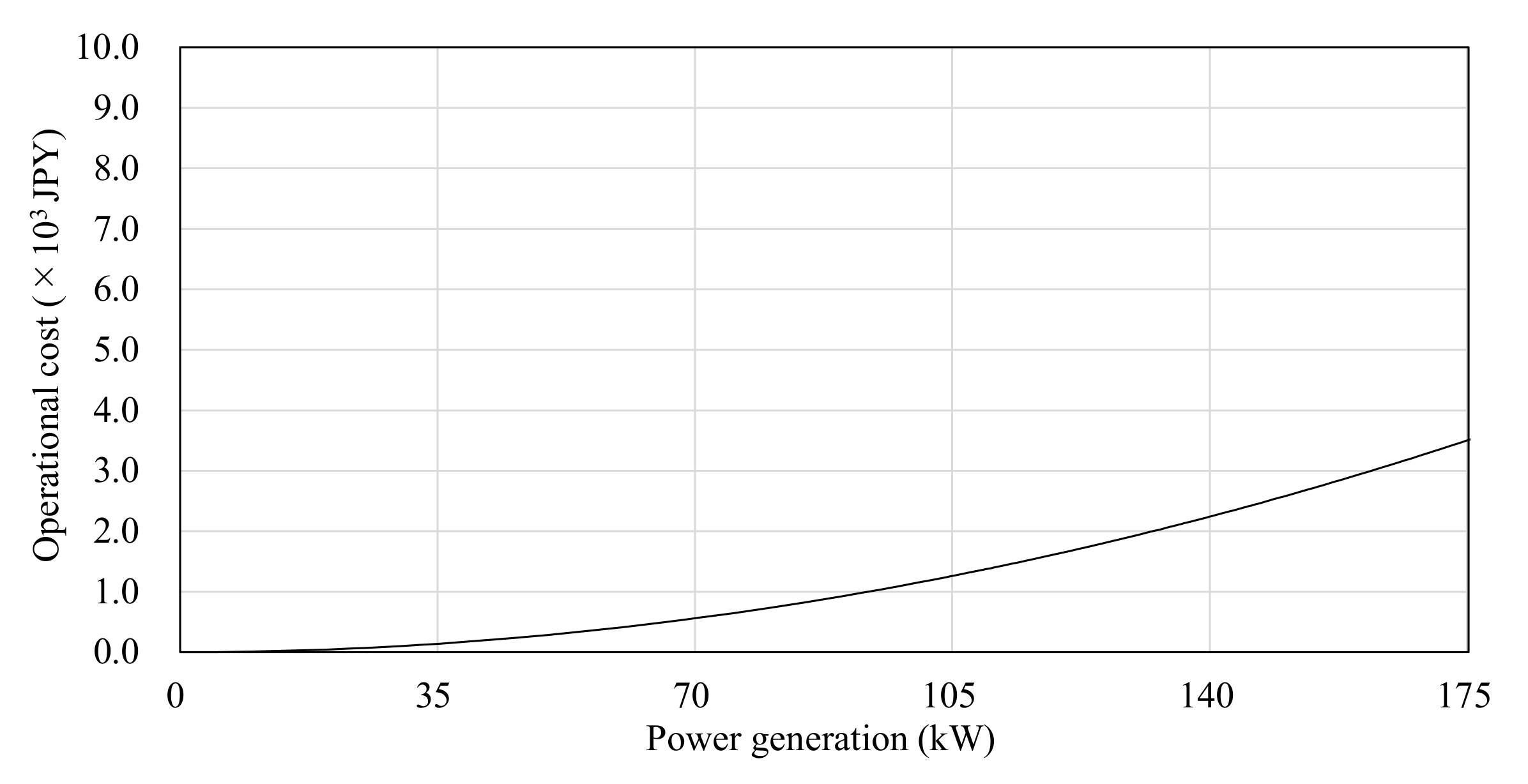
34]. For these reasons, the authors added the following assumptions to make the operational cost function.
Assumption 2. Total operational cost in the power supply is approximated as the quadratic function relying on the fuel costs of thermal power units.
Assumption 3. The power suppliers decide the electricity price to maximize their utility function at the annual average of electricity consumption (103.94 kW in this paper).
The normalized utility function of the power suppliers was defined as:
where
is the electricity price in the normalized function;
,
, and
are the coefficients for the normalized function.
With reference to [
35,
36], the coefficients of the fuel cost function were set to 2.73 × 10
−7 JPY/kWh
2, 2.27 JPY/kWh, and 1.50 × 10
5 JPY. In addition, the maximum and the minimum outputs of power generation (
and
) were set to 175 kW and zero, respectively, based on the electricity consumption of 500 households in the record. With these values, the coefficients in Equation (28) were assumed to 4.63 × 10
−5/kWh
2, 1.20 × 10
−7/kWh, and 0. Owing to Assumption 3, we can calculate
as:
where
is the annual average of electricity consumption.
By multiplying
on both sides in Equation (29), we can update the coefficients as
and
, and as a result, the functions of the power suppliers’ utility and the operational cost were written as:
where
;
.
Figure 1 displays the resulting operational cost function of the suppliers, and its coefficients are summarized in
Table 1.
4.2. Utility Function for Consumers
The consumers’ satisfaction is assumed by several functions such as logarithmic or sigmoidal functions [
37,
38,
39,
40,
41,
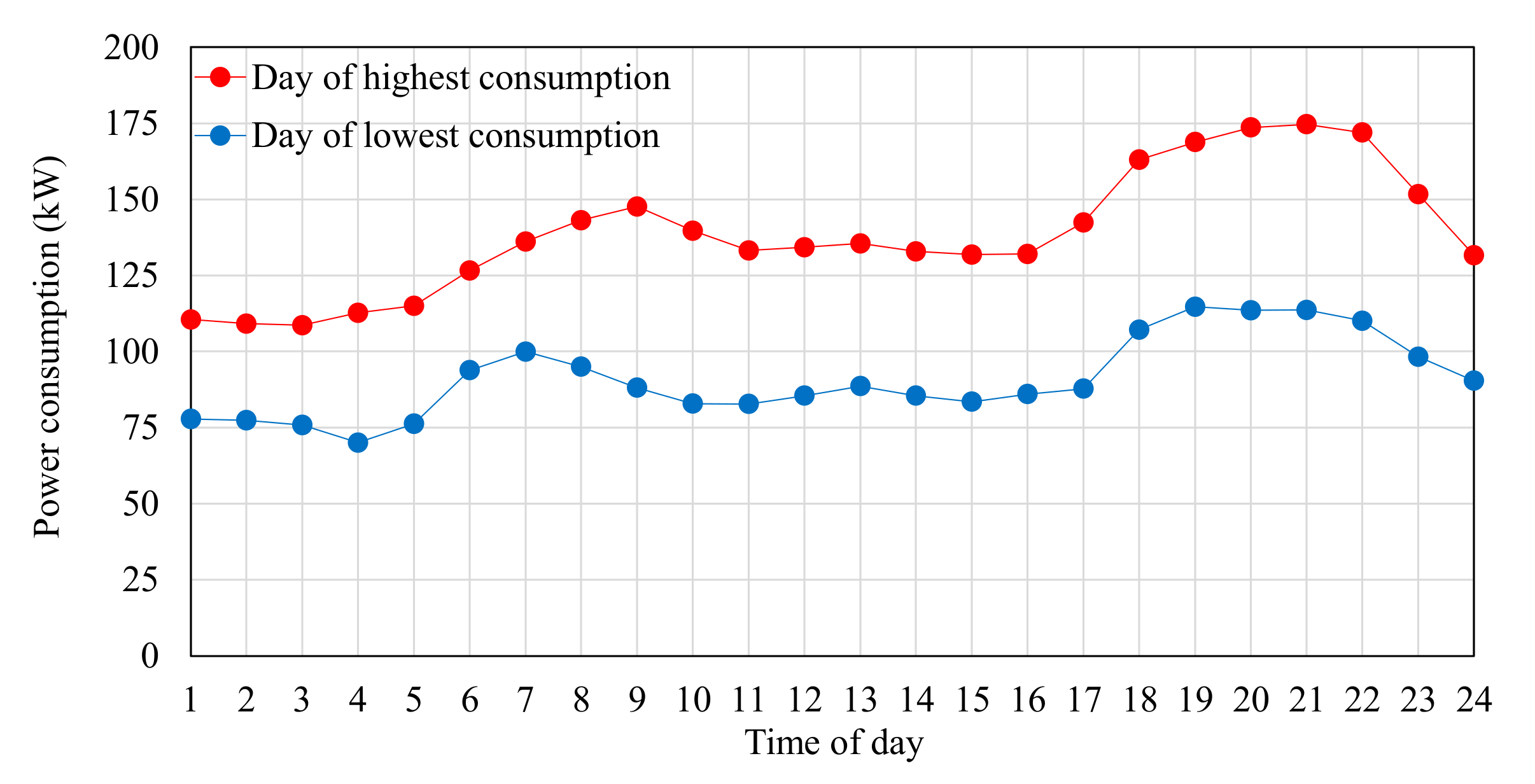
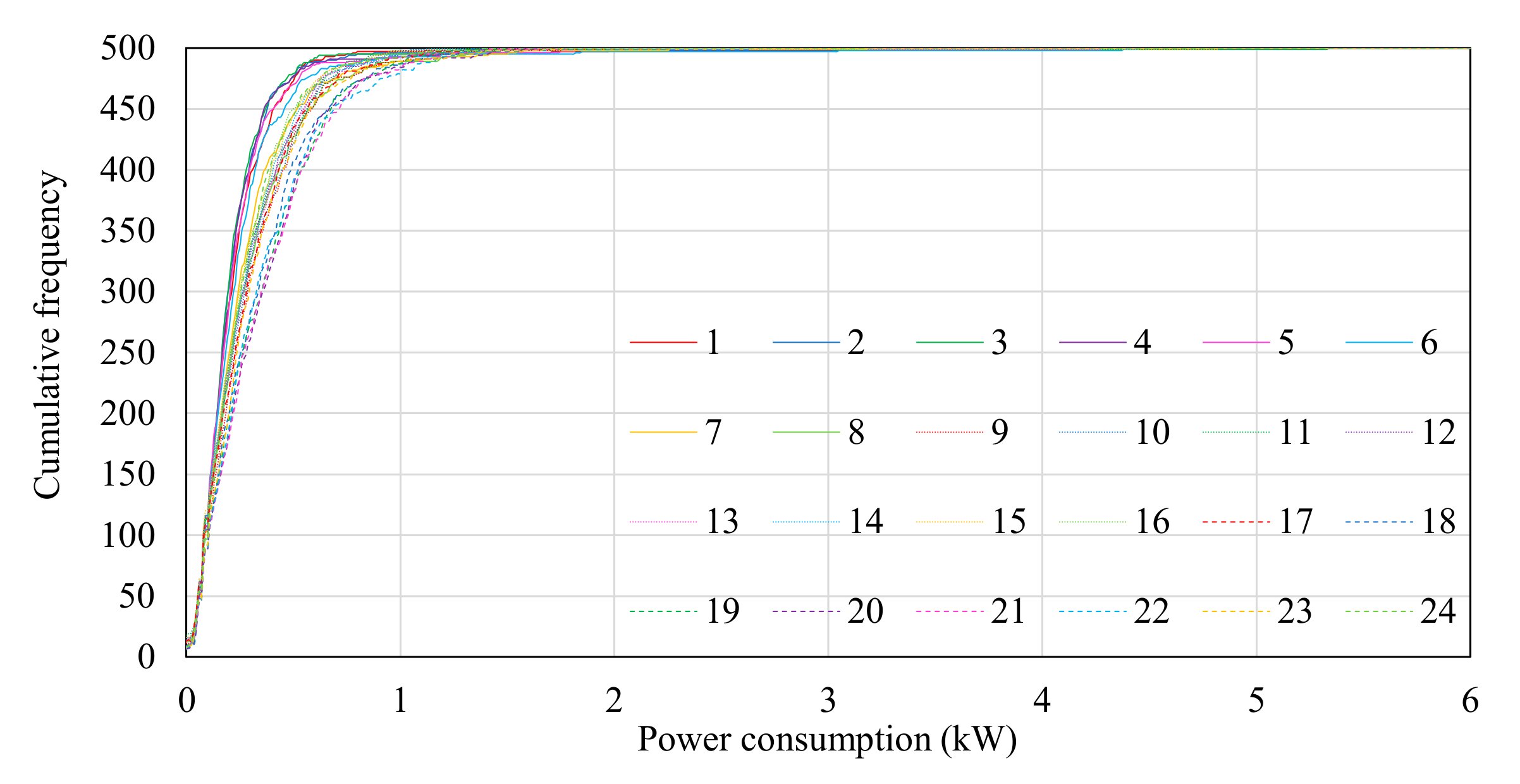
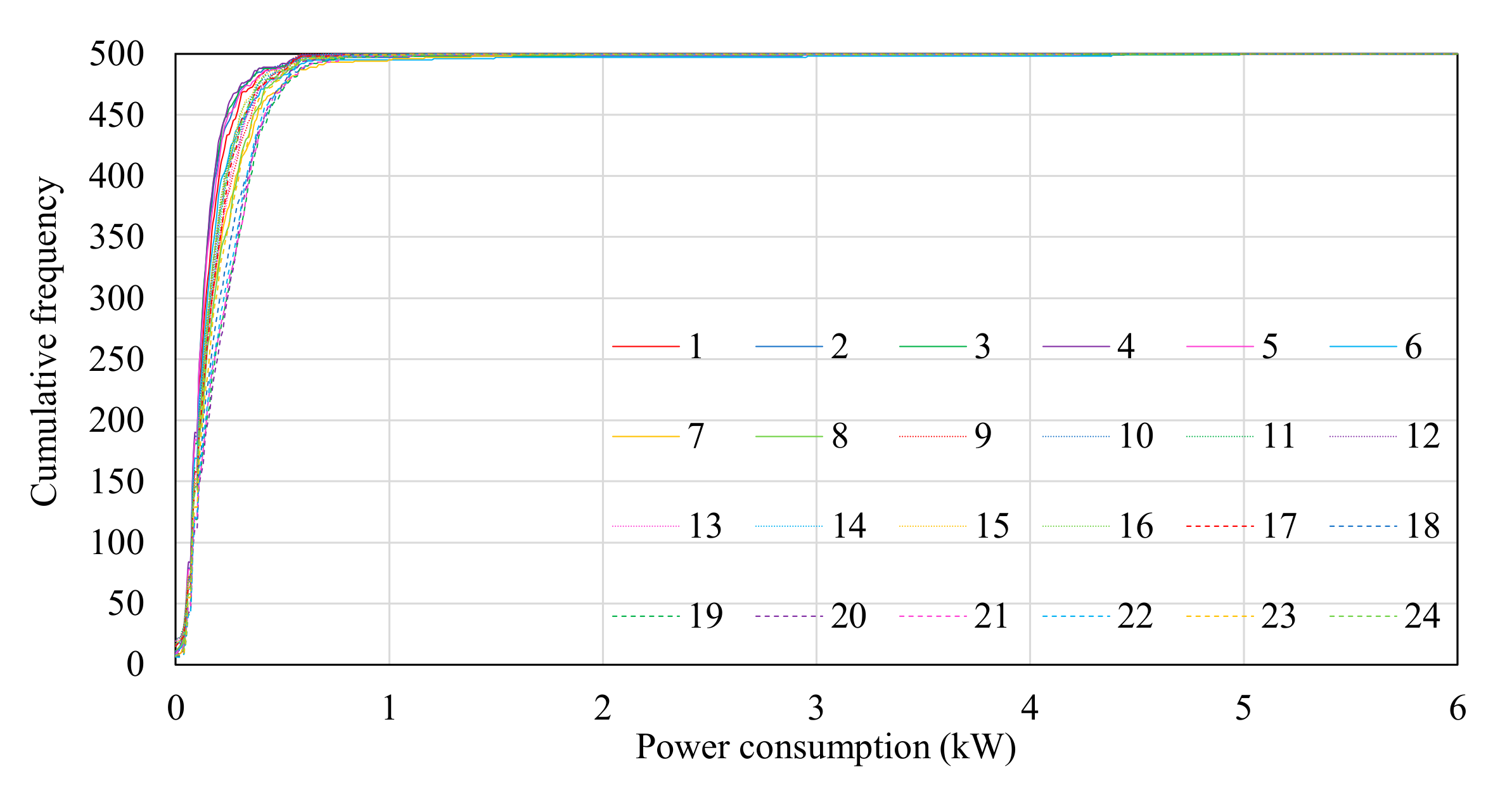
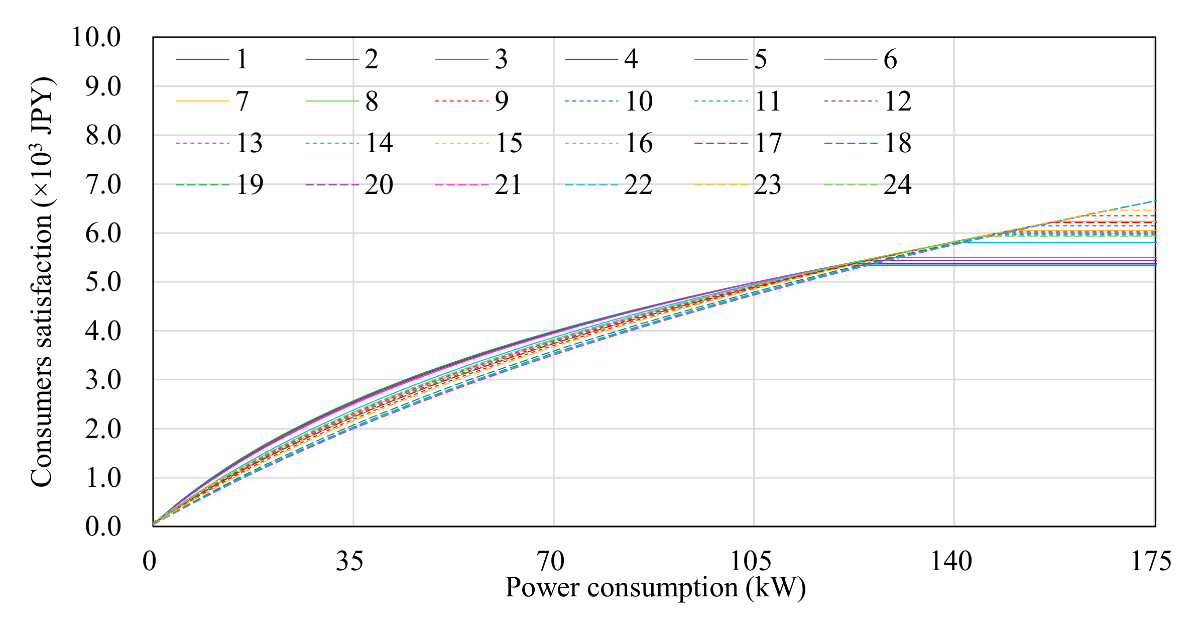
42]. In this paper, the functions of hourly satisfaction were made by relying on the record of smart power meters for 500 households.
Figure 2 shows the profiles of the hourly total electricity consumption of the 500 households, which are samples including the highest or the lowest electricity consumption for one year. The hourly cumulative frequency distributions of the electricity consumption in each household are displayed in
Figure 3 and
Figure 4.
Based on these data, the normalized utility function of the consumers was approximated as:
where
is the electricity price in the normalized function;
,
, and
are the coefficients for the hourly normalized function of consumers’ satisfaction.
Equation (32) suggests how many consumers are satisfied with the electricity consumption
. With assumption 1,
can be calculated as:
As with Equations (30) and (31), we can derive the functions of the consumers’ hourly utility and satisfaction as:
where
;
;
.
5. Numerical Simulation Results
Numerical simulations were carried out with the model constructed in
Section 4. The following scenarios were assumed:
Scenario 1. The power suppliers request to reduce the electricity consumption at any time slot in the day of the highest electricity consumption.
Scenario 2. The power suppliers request to encourage the electricity consumption at any time slot in the day of the lowest electricity consumption.
Under these scenarios, the authors calculated the sets of the optimal electricity price or rebate level and the acceptable condition on each time slot.
5.1. Numerical Simulation Results for Price-Based DRs
By using Equations (18)–(20), the optimal electricity prices and the acceptable conditions in the price-based DR were calculated as:
where
;
.
Table 4 and
Table 5 summarize the calculation results in the case that the power suppliers set the DR target as a 1% decrease (Scenario 1) or increase (Scenario 2) of the standard electricity consumption.
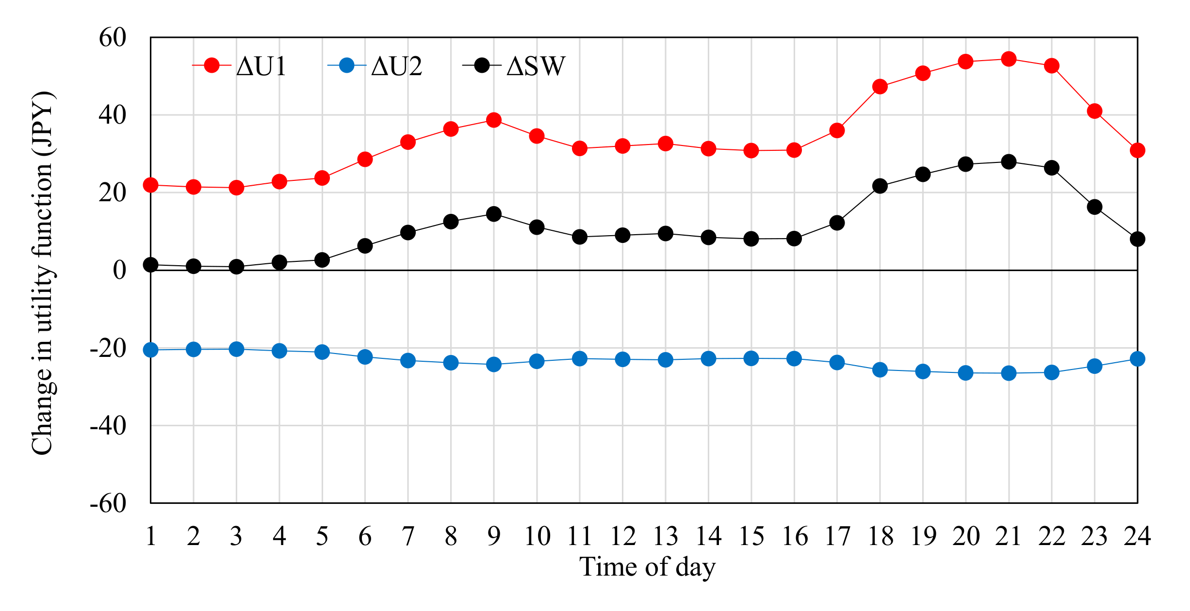
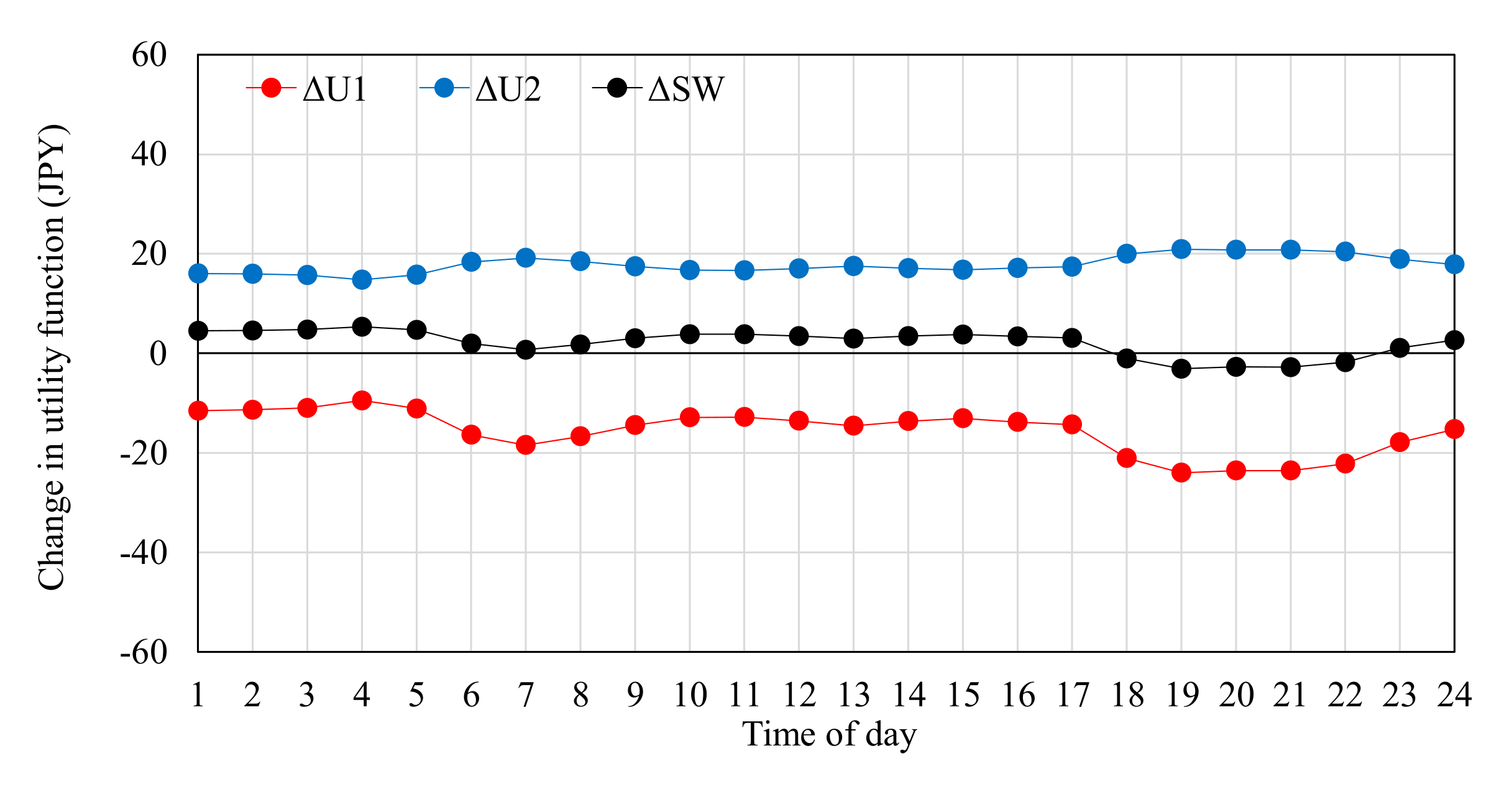
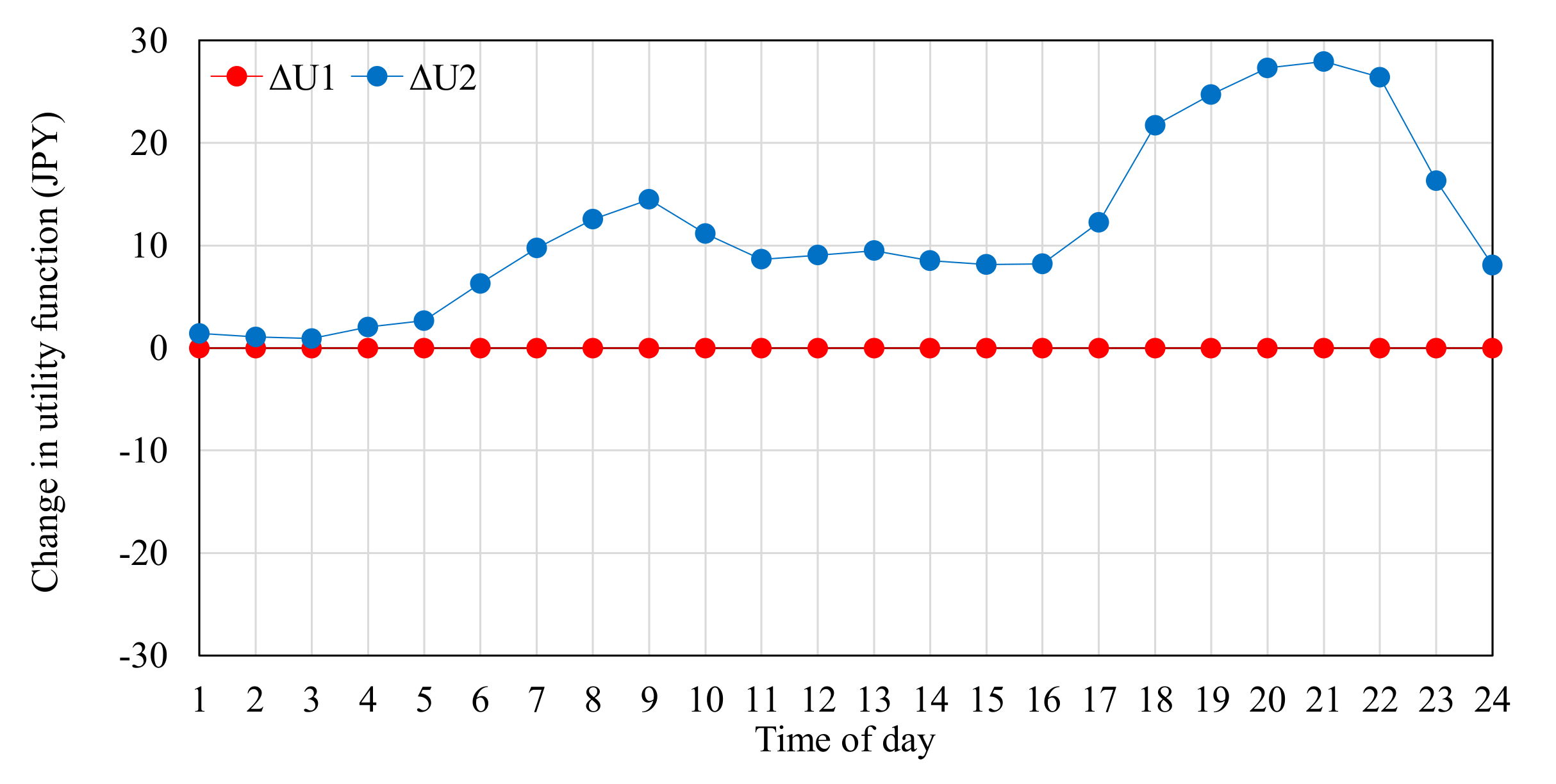
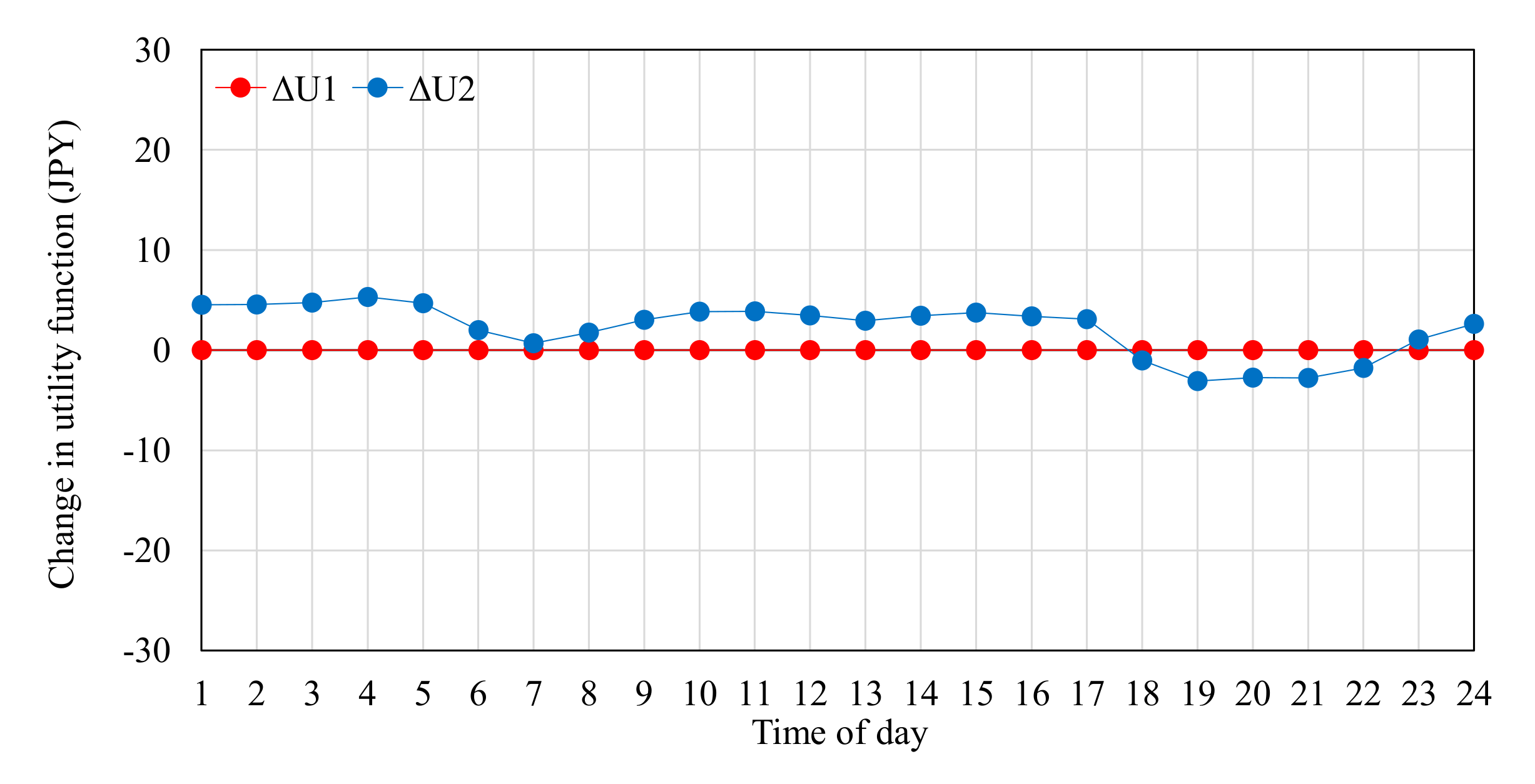
Figure 7 and
Figure 8 illustrate changes in the utility functions of the power suppliers and the consumers and those in the social welfare functions.
In
Table 4, the calculation results in scenario 1 satisfied with their acceptable conditions, and as a result, the optimal electricity prices were slightly increased (less than 1%) as compared to the standard electricity price (23.90 JPY/kWh). By contrast, as shown in
Table 5, the power suppliers could not request a 1% increase in the electricity consumption in scenario 2, because the calculation results did not satisfy their acceptable conditions. In particular, the electricity consumption became higher than its annual average (103.94 kW) from 18:00 to 22:00, and therefore,
exceeded the standard price. In the other periods, the power suppliers can request the DR cooperation, until the condition shown in Equation (38) is violated. With reference to
Figure 2 we can understand that the calculated electricity prices changed inversely to the profile of electricity consumption in
Table 4, while synchronously in
Table 5. These results indicated that the consumers can reduce the power demand during the peak periods, and it becomes difficult in the off-peak periods. That is, the calculated prices reflected the controllability in the electricity consumption on each time slot.
In
Figure 7 and
Figure 8, there were no significant differences in the social welfare by the DR; however, we can confirm that the price-based DRs took burden on the consumers in
Figure 7 or the suppliers in
Figure 8. As displayed in
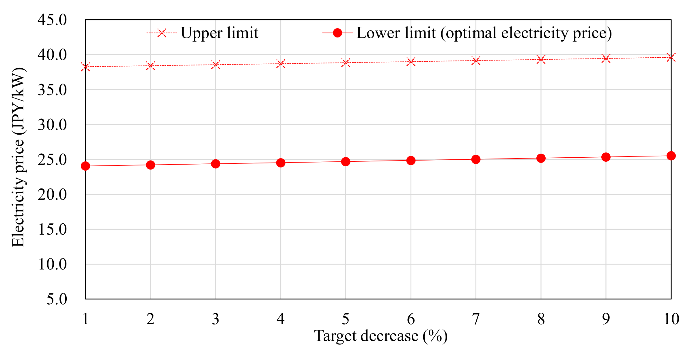
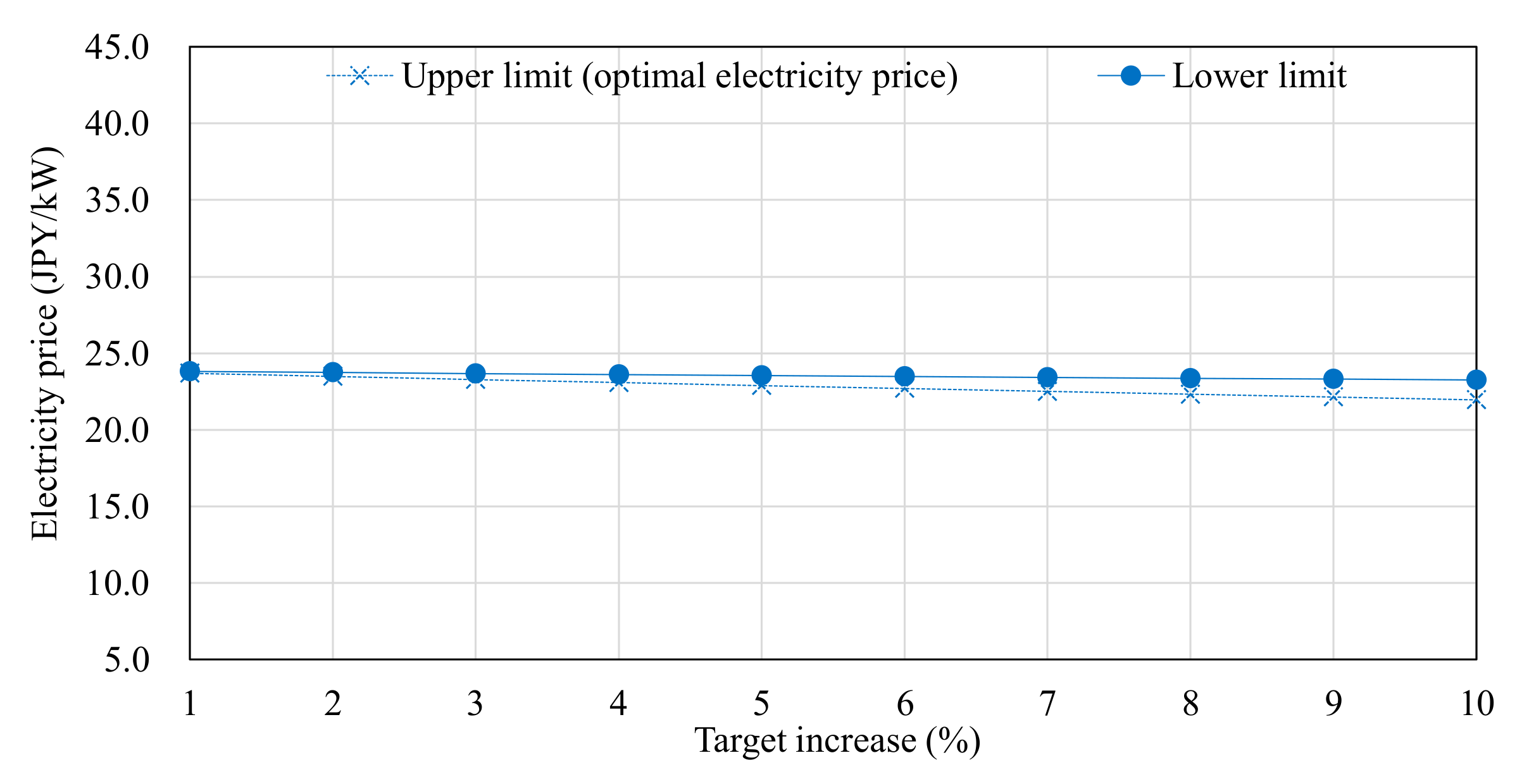
Figure 9, the optimal electricity price became 25.01 JPY/kWh, and the increment of the price exceeded 1 JPY/kWh when the DR target was set to 7% of the actual electricity consumption. As for the reference, the optimal electricity price in scenario 2 is shown in
Figure 10.
In the numerical simulation model, the authors made the operational cost function of the power suppliers relying on the fuel costs of thermal power units. However, in the actual operations, the other factors such as the surplus power of renewable energy sources have influences on the operational cost. If we reflect them appropriately in the model, the results in scenario 2 can be activated.
From these results, the authors concluded that the authors’ proposal functioned properly in the price-based DR.
5.2. Numerical Simulation Results for Incentive-Based DRs
By using Equations (25) and (26), the optimal rebate levels and the acceptable conditions in the incentive-based DR were calculated as:
where
.
Table 6 and
Table 7 summarize the calculation results in the case that the power suppliers set the DR target as a 1% decrease (Scenario 1) or increase (Scenario 2) of the standard electricity consumption.
Figure 11 and
Figure 12 illustrate changes in the utility functions of the power suppliers and the consumers. Changes in the social welfare functions were omitted in
Figure 11 and
Figure 12, because they were the same with the changes of the consumers’ utility functions in the authors’ proposal.
In
Table 6, the calculated rebate levels were in the range of 0.95 JPY/kWh to 16.07 JPY/kWh. Meanwhile, the rebate levels in
Table 7 were in the range of −2.61 JPY/kWh to 7.70 JPY/kWh. As opposed to the results of price-based DRs, the time variation in
Table 6 and
Figure 11 had a similar trend to the electricity consumption. As shown in
Table 7 and
Figure 12, the optimal rebate levels were lower than
from 18:00 to 22:00, and thus, the consumers’ utility became negative during the periods. It indicated that the power suppliers could not ensure the resources for the DR, and the DR request was impossible during the periods. In
Figure 11 and
Figure 12, there were no burden on the power suppliers and no decrement in the social welfare excepting the period from 18:00 to 22:00 in scenario 2.
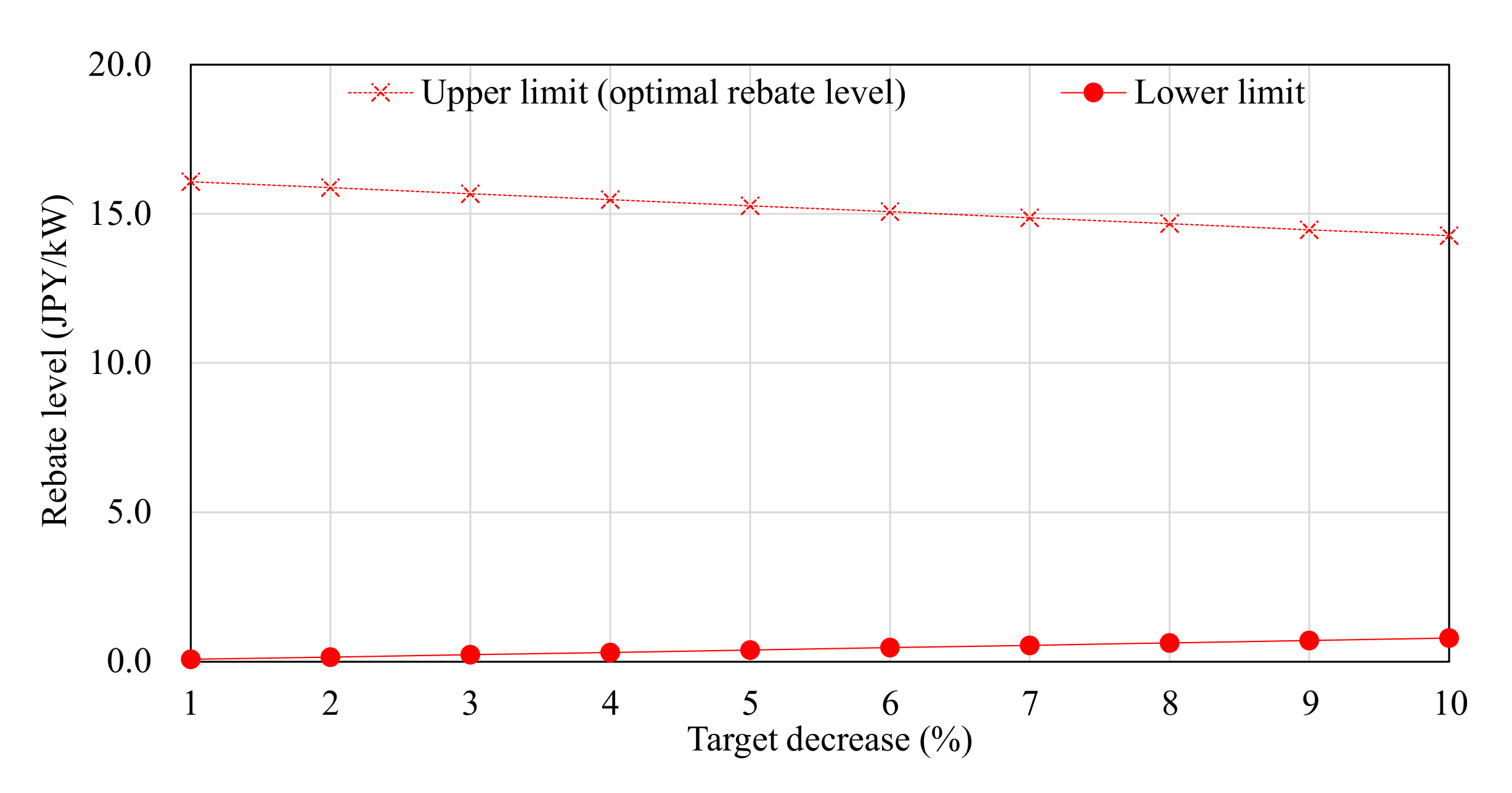
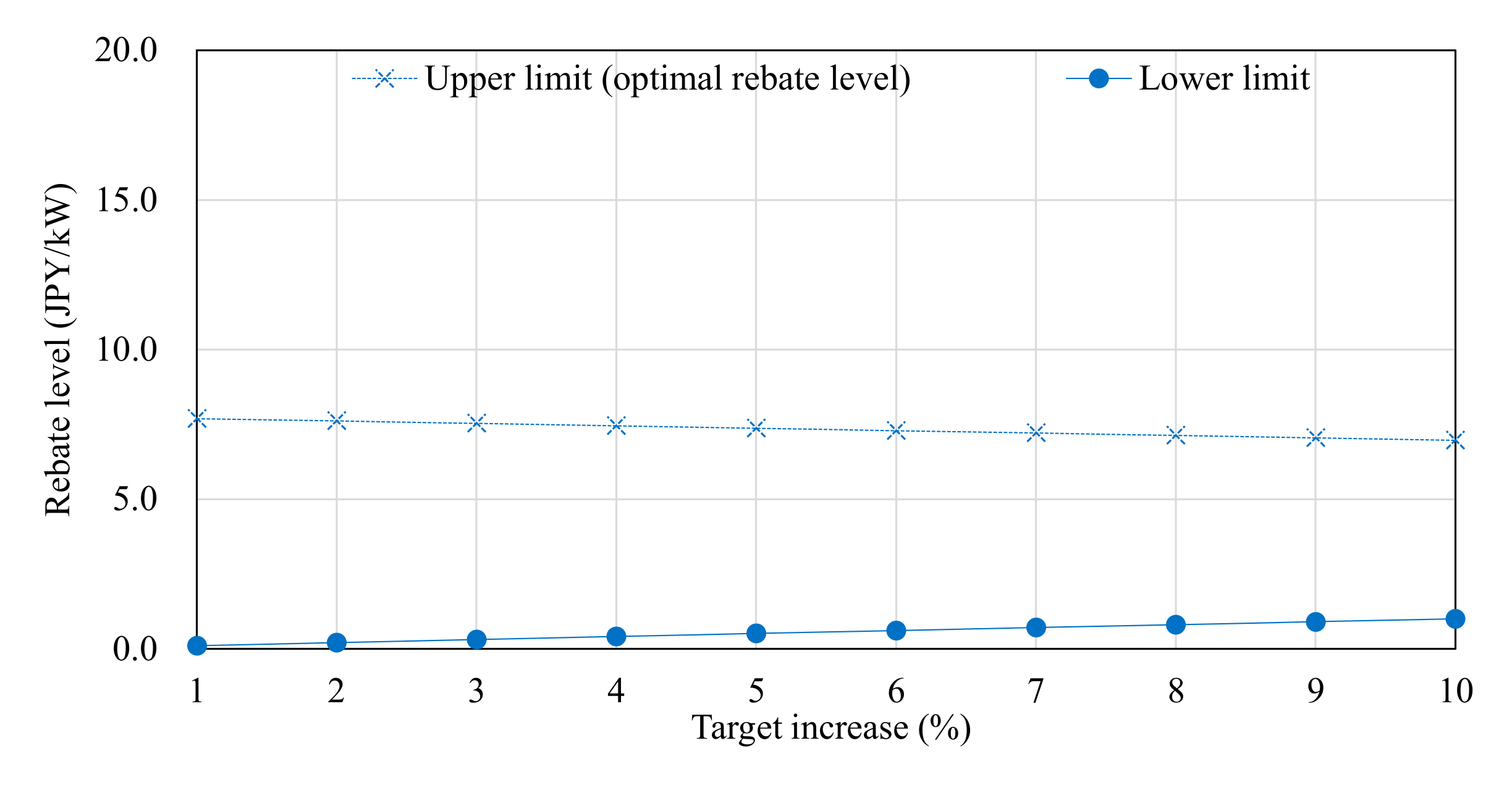
As shown in
Figure 13 and
Figure 14, the optimal rebate levels reduced in response to the decrease (
Figure 13) or increase (
Figure 14) of the target values of the DR. In contrast, the lower limits of the rebate levels were gradually raised. This is because the resources for the DR were limited in association with the utility function of the power suppliers.
These results showed that the authors’ proposal functioned properly in the incentive-based DR as well.
6. Conclusions
The authors proposed a theoretical approach that calculates electricity prices and rebate levels in DRs, based on the framework of SWM. In the authors’ proposal, first, the utility functions of the power suppliers and the consumers were set, and then, the power supply–demand-balancing operation was represented under the SWM framework. Next, the authors derived the acceptable conditions for price-based DRs as Equations (18) and (19) and the acceptable conditions for incentive-based DRs as Equation (25). Besides, the optimal values of electricity prices and rebate levels were defined as Equations (20) and (26), respectively, in consideration of burden on the society. The distinctive feature of the proposed approach was to make influences of the DRs measurable as an increment/decrement in the utility functions. Finally, to verify the validity of the authors’ proposal, the numerical simulations were carried out with the model, which was constructed using the approximated fuel cost function of power generation units and the record of smart power meters.
As shown in
Section 5, the calculated electricity prices and rebate levels became smaller than the values applied in the demonstrative field tests. This is because the calculation results, as defined in Equations (18)–(20) as well as Equations (25) and (26), strongly depended on the utility functions of the power suppliers and the consumers. In other words, the assumed utility functions have room for discussion on their appropriateness. However, the results of the numerical simulations reflected the controllability in electricity consumption, and we can conclude that the authors’ proposal functioned appropriately.
In future works, the appropriateness of the assumed utility functions will be discussed in more detail. Furthermore, the authors will analyze influences of the replacement of the actual electricity consumption, , with the estimated one, and the proposed framework will be expanded.
Author Contributions
Conceptualization, H.T. and N.Y.; methodology, H.T. and N.Y.; software, N.Y.; validation, H.T., N.Y., H.A., A.H. and N.D.T.; writing—original draft preparation, H.T., H.A., A.H. and N.D.T.; writing—review and editing, H.T.; supervision, H.T. and H.A.; project administration, H.T. All authors have read and agreed to the published version of the manuscript.
Funding
This research was partly funded by the Japan Society for the Promotion of Science (JSPS; grant number: 19K04325).
Institutional Review Board Statement
Not applicable.
Informed Consent Statement
Not applicable.
Data Availability Statement
Not applicable.
Conflicts of Interest
The authors declare no conflict of interest.
References
- Palensky, P.; Dietrich, D. Demand Side Management: Demand Response, Intelligent Energy Systems, and Smart Loads. IEEE Trans. Ind. Inform. 2011, 7, 381–388. [Google Scholar] [CrossRef] [Green Version]
- Asano, H.; Nagata, Y. A Survey of Demand Response and Research Activities at CRIEPI. Rev. Electr. Econ. 2015, 62, 1–7. (In Japanese) [Google Scholar]
- Siano, P. Demand Response and Smart Grids—A Survey. Renew. Sustain. Energy Rev. 2014, 30, 461–478. [Google Scholar] [CrossRef]
- Meyabadi, A.F.; Deihimi, M.H. A review of demand-side management: Reconsidering theoretical framework. Renew. Sustain. Energy Rev. 2017, 80, 367–379. [Google Scholar] [CrossRef]
- Albadi, M.; El-Saadany, E. A summary of demand response in electricity markets. Electr. Power Syst. Res. 2008, 78, 1989–1996. [Google Scholar] [CrossRef]
- Deng, R.; Yang, Z.; Chow, M.-Y.; Chen, J. A Survey on Demand Response in Smart Grids: Mathematical Models and Approaches. IEEE Trans. Ind. Inform. 2015, 11, 570–582. [Google Scholar] [CrossRef]
- Vardakas, J.; Zorba, N.; Verikoukis, C.V. A Survey on Demand Response Programs in Smart Grids: Pricing Methods and Optimization Algorithms. IEEE Commun. Surv. Tutor. 2014, 17, 152–178. [Google Scholar] [CrossRef]
- Yan, X.; Ozturk, Y.; Hu, Z.; Song, Y. A review on price-driven residential demand response. Renew. Sustain. Energy Rev. 2018, 96, 411–419. [Google Scholar] [CrossRef]
- Faruqui, A.; Bourbonnais, C. The Tariffs of Tomorrow: Innovations in rate designs. IEEE Power Energy Mag. 2020, 18, 18–25. [Google Scholar] [CrossRef]
- Faruqui, A.; Sergici, S. Household response to dynamic pricing of electricity: A survey of 15 experiments. J. Regul. Econ. 2010, 38, 193–225. [Google Scholar] [CrossRef]
- Heter, K.; Wayland, S. Residential Response to Critical-Peak Pricing of Electricity: California Evidence. Energy 2010, 35, 1561–1567. [Google Scholar] [CrossRef]
- Erucsibm, T. Households’ Self-Selection of Dynamic Electricity Tariffs. Appl. Energy 2011, 88, 2541–2547. [Google Scholar]
- Bartusch, C.; Wallin, F.; Odlare, M.; Vassileva, I.; Wester, L. Introducing a demand-based electricity distribution tariff in the residential sector: Demand response and customer perception. Energy Policy 2011, 39, 5008–5025. [Google Scholar] [CrossRef]
- Yousefi, S.; Nighaddam, M.P.; Majd, V.J. Optimal Real Time Pricing in an Agent-based Retail Market Suing a Compre-hensive Demand Response Model. Energy 2011, 36, 5716–5727. [Google Scholar] [CrossRef]
- Yoon, J.H.; Bladick, R.; Novoselac, A. Demand response for residential buildings based on dynamic price of electricity. Energy Build. 2014, 80, 531–541. [Google Scholar] [CrossRef]
- Kawamura, K.; Doki, T.; Oono, Y.; Takano, H.; Murata, J. Analysis of Field Test Results and Proposal of Sustainable De-mand Peak Reduction in Demand Response Programs for Residential Consumers. IEEJ Trans. Electron. Inf. Syst. 2017, 137, 96–105. (In Japanese) [Google Scholar]
- Zou, X. Double-sided auction mechanism design in electricity based on maximizing social welfare. Energy Policy 2009, 37, 4231–4239. [Google Scholar] [CrossRef]
- Yang, P.; Tang, G.; Nehorai, A. A game-theoretic approach for optimal time-of-use electricity pricing. IEEE Trans. Power Syst. 2012, 28, 884–892. [Google Scholar] [CrossRef]
- Li, N.; Chen, L.; Dahleh, M.A. Demand Response Using Linear Supply Function Bidding. IEEE Trans. Smart Grid 2015, 6, 1827–1838. [Google Scholar] [CrossRef]
- Hase, R.; Shinomiya, N. A mathematical modeling technique with network flows for social welfare maximization in deregulated electricity markets. Oper. Res. Perspect. 2016, 3, 59–66. [Google Scholar] [CrossRef] [Green Version]
- Sorin, E.; Bobo, L.; Pinson, P. Consensus-Based Approach to Peer-to-Peer Electricity Markets with Product Differentiation. IEEE Trans. Power Syst. 2018, 34, 994–1004. [Google Scholar] [CrossRef] [Green Version]
- Luenberger, D.G. Microeconomics Theory; McGraw-Hill: New York, NY, USA, 1995. [Google Scholar]
- Perloff, J.M. Microeconomics, 2nd ed.; Addison-Wesley: Boston, MA, USA, 2001. [Google Scholar]
- Hausman, D.; McPherson, M.; Sats, D. Economic Analysis, Moral Philosophy, and Public Policy, 3rd ed.; Cambridge University Press: Cambridge, UK, 2016. [Google Scholar]
- Liu, H.; Shen, Y.; Zabinsky, Z.B.; Liu, C.C.; Courts, A.; Joo, S.K. Social Welfare Maximization in Transmission Enhance-ment Considering Network Congestion. IEEE Trans. Power Syst. 2008, 23, 1105–1114. [Google Scholar]
- Baharlouei, Z.; Hashemi, M.; Narimani, H.; Mohsenian-Rad, H. Achieving Optimality and Fairness in Autonomous De-mand Response: Benchmarks and Billing Mechanisms. IEEE Trans. Smart Grid 2013, 4, 968–975. [Google Scholar] [CrossRef]
- Wang, H.; Gao, Y. Real-time pricing method for smart grids based on complementarity problem. J. Mod. Power Syst. Clean Energy 2019, 7, 1280–1293. [Google Scholar] [CrossRef] [Green Version]
- Agency for Natural Resources and Energy. Japan’s Energy White Paper. 2020. Available online: https://www.enecho.meti.go.jp/about/whitepaper/ (accessed on 31 May 2021).
- Hobbs, B.F.; Rothkopf, M.H.; O’Neill, R.P.; Chao, H.P. The Next Generation of Electric Power Unit Commitment Models; Springer: Singapore, 2001; Volume 36. [Google Scholar]
- Padhy, N.P. Unit Commitment—A Bibliographical Survey. IEEE Trans. Power Syst. 2004, 19, 1196–1205. [Google Scholar] [CrossRef]
- Saravanan, B.C.; Das, S.; Sikri, S.; Kothari, D.P. A solution to the unit commitment problem—A review. Front. Energy 2013, 7, 223–236. [Google Scholar] [CrossRef]
- Zheng, Q.; Wang, J.; Liu, A.L. Stochastic Optimization for Unit Commitment—A Review. IEEE Trans. Power Syst. 2014, 30, 1913–1924. [Google Scholar] [CrossRef]
- Takano, H.; Asano, H.; Gupta, N. Application Example of Particle Swarm Optimization on Operation Scheduling of Mi-crogrids. In Frontier Applications of Nature Inspired Computation; Khosravy, M., Gupta, N., Patel, N., Senju, T., Eds.; Springer: Singapore, 2020; pp. 967–994. [Google Scholar]
- Takano, H.; Goto, R.; Hayashi, R.; Asano, H. Optimization Method for Operation Schedule of Microgrids Considering Uncertainty in Available Data. Energies 2021, 14, 2487. [Google Scholar] [CrossRef]
- Investigation R&D Committee on IEEJ. Electrical Power System Standard Models; IEEJ: Tokyo, Japan, 1999; Volume 754. (In Japanese) [Google Scholar]
- Uchida, N.; Kawata, K.; Egawa, M. Development of test case models for Japanese power systems. In Proceedings of the 2000 Power Engineering Society Summer Meeting, Seattle, WA, USA, 16–20 July 2000. [Google Scholar] [CrossRef]
- Wang, L.; Wang, Z.; Yang, R. Intelligent Multiagent Control System for Energy and Comfort Management in Smart and Sustainable Buildings. IEEE Trans. Smart Grid 2012, 3, 605–617. [Google Scholar] [CrossRef]
- Liu, Y.; Zhang, Y.; Chen, K.; Chen, S.Z.; Tang, B. Equivalence of Multi-Time Scale Optimization for Home Energy Man-agement Considering User Discomfort Preference. IEEE Trans. Smart Grid 2017, 8, 1876–1887. [Google Scholar] [CrossRef]
- Li, D.; Chiu, W.-Y.; Sun, H.; Poor, H.V. Multiobjective Optimization for Demand Side Management Program in Smart Grid. IEEE Trans. Ind. Inform. 2017, 14, 1482–1490. [Google Scholar] [CrossRef] [Green Version]
- Takano, H.; Kudo, A.; Taoka, H.; Ohara, A. A basic study on incentive pricing for demand response programs based on social welfare maximization. J. Int. Counc. Electr. Eng. 2018, 8, 136–144. [Google Scholar] [CrossRef] [Green Version]
- Takano, H.; Tanonaka, N.; Kikuda, S.; Ohara, A. A Design Method for Incentive-based Demand Response Programs Based on a Framework of Social Welfare Maximization. IFAC-PapersOnLine 2018, 51, 374–379. [Google Scholar]
- Patnam, B.S.K.; Pindoriya, N.M. Demand response in consumer-Centric electricity market: Mathematical models and optimization problems. Electr. Power Syst. Res. 2021, 193, 106923. [Google Scholar] [CrossRef]
Figure 1.
Operational cost function.
Figure 1.
Operational cost function.
Figure 2.
Example of profiles of hourly electricity consumption.
Figure 2.
Example of profiles of hourly electricity consumption.
Figure 3.
Hourly cumulative frequency distributions in the day of the highest electricity consumption.
Figure 3.
Hourly cumulative frequency distributions in the day of the highest electricity consumption.
Figure 4.
Hourly cumulative frequency distributions in the day of the lowest electricity consumption.
Figure 4.
Hourly cumulative frequency distributions in the day of the lowest electricity consumption.
Figure 5.
Hourly satisfaction functions in the day of the highest electricity consumption.
Figure 5.
Hourly satisfaction functions in the day of the highest electricity consumption.
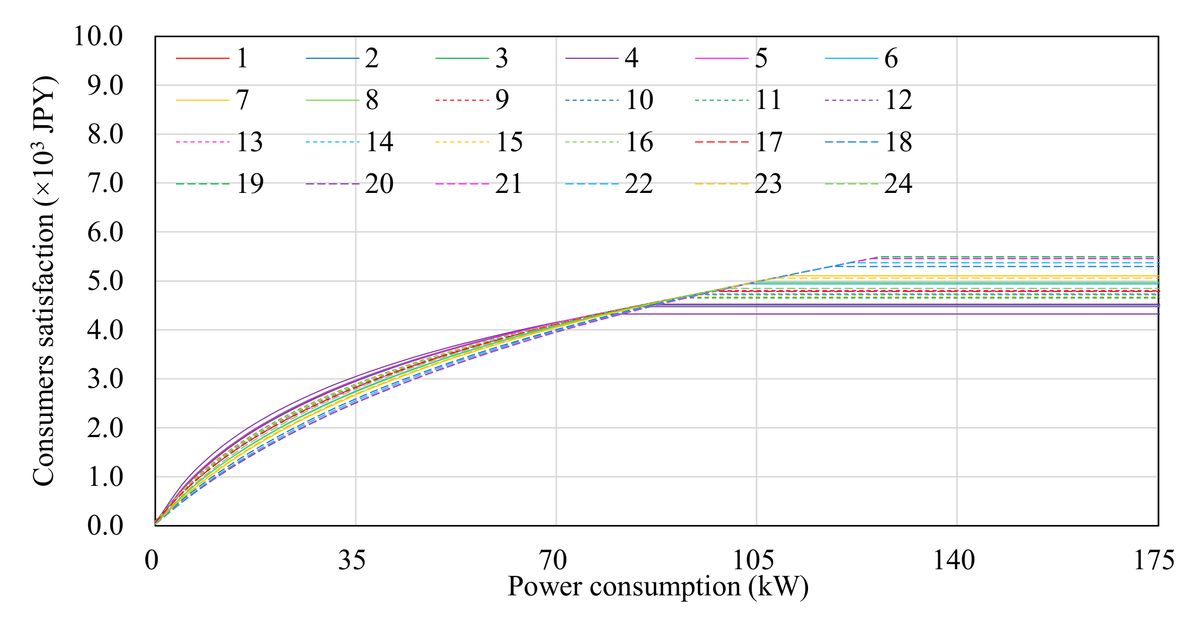
Figure 6.
Hourly satisfaction functions in the day of the lowest electricity consumption.
Figure 6.
Hourly satisfaction functions in the day of the lowest electricity consumption.
Figure 7.
Changes in each function by the 1% DR request in the day of the highest electricity consumption.
Figure 7.
Changes in each function by the 1% DR request in the day of the highest electricity consumption.
Figure 8.
Changes in each function by the 1% DR request in the day of the lowest electricity consumption. In this scenario, the power suppliers could not request the DR cooperation in the target period.
Figure 8.
Changes in each function by the 1% DR request in the day of the lowest electricity consumption. In this scenario, the power suppliers could not request the DR cooperation in the target period.
Figure 9.
Results on the typical time slots in scenario 1 (at 22:00).
Figure 9.
Results on the typical time slots in scenario 1 (at 22:00).
Figure 10.
Results on the typical time slots in scenario 2 (at 4:00). In this scenario, the power suppliers could not request the DR cooperation in the target period.
Figure 10.
Results on the typical time slots in scenario 2 (at 4:00). In this scenario, the power suppliers could not request the DR cooperation in the target period.
Figure 11.
Changes in each function by the 1% DR request in the day of the highest electricity consumption.
Figure 11.
Changes in each function by the 1% DR request in the day of the highest electricity consumption.
Figure 12.
Changes in each function by the 1% DR request in the day of the lowest electricity consumption. In this scenario, the power suppliers could not request the DR cooperation from 18:00 to 22:00.
Figure 12.
Changes in each function by the 1% DR request in the day of the lowest electricity consumption. In this scenario, the power suppliers could not request the DR cooperation from 18:00 to 22:00.
Figure 13.
Results on the typical time slots in scenario 1 (at 22:00).
Figure 13.
Results on the typical time slots in scenario 1 (at 22:00).
Figure 14.
Results on the typical time slots in scenario 2 (at 4:00). In this scenario, the power suppliers could not request the DR cooperation from 18:00 to 22:00.
Figure 14.
Results on the typical time slots in scenario 2 (at 4:00). In this scenario, the power suppliers could not request the DR cooperation from 18:00 to 22:00.
| A (×10−1 JPY/kWh2) | B (×10−4 JPY/kWh) | C (JPY) |
|---|
| 1.15 | 2.99 | 0 |
Table 2.
Coefficients in
Figure 5 (the day of the highest electricity consumption).
Table 2.
Coefficients in
Figure 5 (the day of the highest electricity consumption).
| | | | | | | |
|---|
| 1 | 3.41 | 3.16 | 32.03 | 13 | 4.55 | 1.85 | 54.75 |
| 2 | 3.35 | 3.25 | 31.15 | 14 | 4.44 | 1.93 | 52.78 |
| 3 | 3.32 | 3.32 | 30.41 | 15 | 4.39 | 1.97 | 51.77 |
| 4 | 3.50 | 2.99 | 33.77 | 16 | 4.39 | 1.97 | 51.47 |
| 5 | 3.60 | 2.84 | 35.59 | 17 | 4.89 | 1.63 | 62.21 |
| 6 | 4.11 | 2.22 | 45.55 | 18 | 5.93 | 1.18 | 85.10 |
| 7 | 4.56 | 1.85 | 54.56 | 19 | 6.25 | 1.08 | 92.87 |
| 8 | 4.92 | 1.61 | 62.80 | 20 | 6.52 | 1.02 | 99.01 |
| 9 | 5.15 | 1.49 | 67.62 | 21 | 6.58 | 1.00 | 100.57 |
| 10 | 4.76 | 1.71 | 59.44 | 22 | 6.43 | 1.04 | 97.03 |
| 11 | 4.46 | 1.91 | 53.44 | 23 | 5.34 | 1.40 | 71.73 |
| 12 | 4.49 | 1.89 | 53.69 | 24 | 4.35 | 2.01 | 50.33 |
Table 3.
Coefficients in
Figure 6 (the day of the lowest electricity consumption).
Table 3.
Coefficients in
Figure 6 (the day of the lowest electricity consumption).
| | | | | | | |
|---|
| 1 | 2.15 | 8.38 | 12.13 | 13 | 2.56 | 5.65 | 18.38 |
| 2 | 2.14 | 8.47 | 12.09 | 14 | 2.44 | 6.29 | 16.42 |
| 3 | 2.08 | 9.03 | 11.29 | 15 | 2.36 | 6.72 | 15.42 |
| 4 | 1.89 | 11.40 | 9.03 | 16 | 2.45 | 6.20 | 16.62 |
| 5 | 2.10 | 8.90 | 11.43 | 17 | 2.52 | 5.85 | 17.59 |
| 6 | 2.74 | 4.92 | 20.63 | 18 | 3.28 | 3.40 | 29.87 |
| 7 | 2.97 | 4.14 | 24.45 | 19 | 3.58 | 2.87 | 35.21 |
| 8 | 2.79 | 4.72 | 21.59 | 20 | 3.53 | 2.95 | 34.27 |
| 9 | 2.53 | 5.80 | 17.77 | 21 | 3.54 | 2.93 | 34.57 |
| 10 | 2.34 | 6.90 | 14.97 | 22 | 3.38 | 3.20 | 31.49 |
| 11 | 2.34 | 6.87 | 15.15 | 23 | 2.91 | 4.34 | 23.33 |
| 12 | 2.44 | 6.26 | 16.64 | 24 | 2.60 | 5.47 | 18.54 |
Table 4.
Numerical simulation results of price-based demand response programs (DRs) under scenario 1.
Table 4.
Numerical simulation results of price-based demand response programs (DRs) under scenario 1.
| | | | | |
|---|
| 1 | 24.09 | 46.61 | 13 | 24.07 | 42.42 |
| 2 | 24.09 | 46.88 | 14 | 24.07 | 42.79 |
| 3 | 24.09 | 47.00 | 15 | 24.07 | 42.93 |
| 4 | 24.09 | 46.15 | 16 | 24.07 | 42.90 |
| 5 | 24.08 | 45.71 | 17 | 24.07 | 41.52 |
| 6 | 24.08 | 43.72 | 18 | 24.06 | 39.29 |
| 7 | 24.07 | 42.33 | 19 | 24.06 | 38.76 |
| 8 | 24.07 | 41.43 | 20 | 24.05 | 38.35 |
| 9 | 24.07 | 40.89 | 21 | 24.05 | 38.26 |
| 10 | 24.07 | 41.86 | 22 | 24.05 | 38.49 |
| 11 | 24.07 | 42.74 | 23 | 24.06 | 40.43 |
| 12 | 24.07 | 42.59 | 24 | 24.07 | 42.96 |
Table 5.
Numerical simulation results of price-based DRs under scenario 2.
Table 5.
Numerical simulation results of price-based DRs under scenario 2.
| | | | | |
|---|
| 1 | 23.84 | 23.69 | 13 | 23.87 | 23.70 |
| 2 | 23.84 | 23.70 | 14 | 23.86 | 23.70 |
| 3 | 23.84 | 23.69 | 15 | 23.85 | 23.70 |
| 4 | 23.82 | 23.69 | 16 | 23.86 | 23.70 |
| 5 | 23.84 | 23.69 | 17 | 23.86 | 23.70 |
| 6 | 23.88 | 23.71 | 18 | 23.91 | 23.71 |
| 7 | 23.89 | 23.71 | 19 | 23.93 | 23.72 |
| 8 | 23.88 | 23.71 | 20 | 23.92 | 23.72 |
| 9 | 23.86 | 23.70 | 21 | 23.92 | 23.72 |
| 10 | 23.85 | 23.70 | 22 | 23.92 | 23.72 |
| 11 | 23.85 | 23.70 | 23 | 23.89 | 23.71 |
| 12 | 23.86 | 23.70 | 24 | 23.87 | 23.70 |
Table 6.
Numerical simulation results of incentive-based DRs under scenario 1.
Table 6.
Numerical simulation results of incentive-based DRs under scenario 1.
| | | | | |
|---|
| 1 | 9.31 | 1.38 | 13 | 8.55 | 7.10 |
| 2 | 9.35 | 1.08 | 14 | 8.59 | 6.50 |
| 3 | 9.38 | 0.95 | 15 | 8.62 | 6.26 |
| 4 | 9.24 | 1.90 | 16 | 8.64 | 6.31 |
| 5 | 9.17 | 2.42 | 17 | 8.36 | 8.68 |
| 6 | 8.83 | 5.06 | 18 | 7.89 | 13.40 |
| 7 | 8.57 | 7.24 | 19 | 7.74 | 14.72 |
| 8 | 8.34 | 8.85 | 20 | 7.64 | 15.81 |
| 9 | 8.23 | 9.89 | 21 | 7.62 | 16.07 |
| 10 | 8.42 | 8.06 | 22 | 7.67 | 15.43 |
| 11 | 8.57 | 6.57 | 23 | 8.15 | 10.83 |
| 12 | 8.58 | 6.82 | 24 | 8.69 | 6.23 |
Table 7.
Numerical simulation results of incentive-based DRs under scenario 2.
Table 7.
Numerical simulation results of incentive-based DRs under scenario 2.
| | | | | |
|---|
| 1 | 10.28 | 5.90 | 13 | 9.84 | 3.41 |
| 2 | 10.28 | 6.00 | 14 | 9.97 | 4.14 |
| 3 | 10.34 | 6.37 | 15 | 10.03 | 4.60 |
| 4 | 10.52 | 7.70 | 16 | 9.96 | 4.02 |
| 5 | 10.33 | 6.27 | 17 | 9.90 | 3.62 |
| 6 | 9.74 | 2.22 | 18 | 9.30 | −0.88 |
| 7 | 9.55 | 0.80 | 19 | 9.10 | −2.61 |
| 8 | 9.68 | 1.94 | 20 | 9.13 | −2.33 |
| 9 | 9.89 | 3.55 | 21 | 9.12 | −2.36 |
| 10 | 10.07 | 4.75 | 22 | 9.24 | −1.53 |
| 11 | 10.04 | 4.77 | 23 | 9.61 | 1.19 |
| 12 | 9.95 | 4.15 | 24 | 9.86 | 3.01 |
| Publisher’s Note: MDPI stays neutral with regard to jurisdictional claims in published maps and institutional affiliations. |
© 2021 by the authors. Licensee MDPI, Basel, Switzerland. This article is an open access article distributed under the terms and conditions of the Creative Commons Attribution (CC BY) license (https://creativecommons.org/licenses/by/4.0/).


 and
and 


