Data-Driven Reinforcement-Learning-Based Automatic Bucket-Filling for Wheel Loaders

Abstract

Automation of bucket-filling is of crucial significance to the fully automated systems for wheel loaders. Most previous works are based on a physical model, which cannot adapt to the changeable and complicated working environment. Thus, in this paper, a data-driven reinforcement-learning (RL)-based approach is proposed to achieve automatic bucket-filling. An automatic bucket-filling algorithm based on Q-learning is developed to enhance the adaptability of the autonomous scooping system. A nonlinear, non-parametric statistical model is also built to approximate the real working environment using the actual data obtained from tests. The statistical model is used for predicting the state of wheel loaders in the bucket-filling process. Then, the proposed algorithm is trained on the prediction model. Finally, the results of the training confirm that the proposed algorithm has good performance in adaptability, convergence, and fuel consumption in the absence of a physical model. The results also demonstrate the transfer learning capability of the proposed approach. The proposed method can be applied to different machine-pile environments.

1. Introduction

Construction machinery has a pivotal role in the building and mining industry, which makes a great contribution to the world economy [1]. The wheel loader is one of the most common mobile construction machinery and is often used to transport different materials at production sites [2].

The automation of wheel loaders, which has received great attention over the past three decades, can improve safety and reduce costs. Dadhich et al. [3] proposed five steps to full automation of wheel loaders: manual operation, in-sight tele-operation, tele-remote operation, assisted tele-remote operation, and fully autonomous operation. Despite extensive research in this field, fully automated systems for wheel loaders have never been demonstrated. Remote operation is considered a step towards fully automated equipment, but it has led to a reduction in productivity and fuel efficiency [4].

In the working process of wheel loaders, bucket-filling is a crucial part, as it determines the weight of the loaded materials. Bucket-filling is a relatively repetitive task for the operators of wheel-loaders and is suitable for automation. Automatic bucket-filling is also required for efficient remote operation and the development of fully autonomous solutions [5]. The interaction condition between the bucket and the pile strongly affects the bucket-filling. However, due to the complexity of the working environment, the interaction condition is unknown and constantly changing. The difference in working materials also influences the bucket-filling. A general automatic bucket-filling solution is still a challenge for different piles.

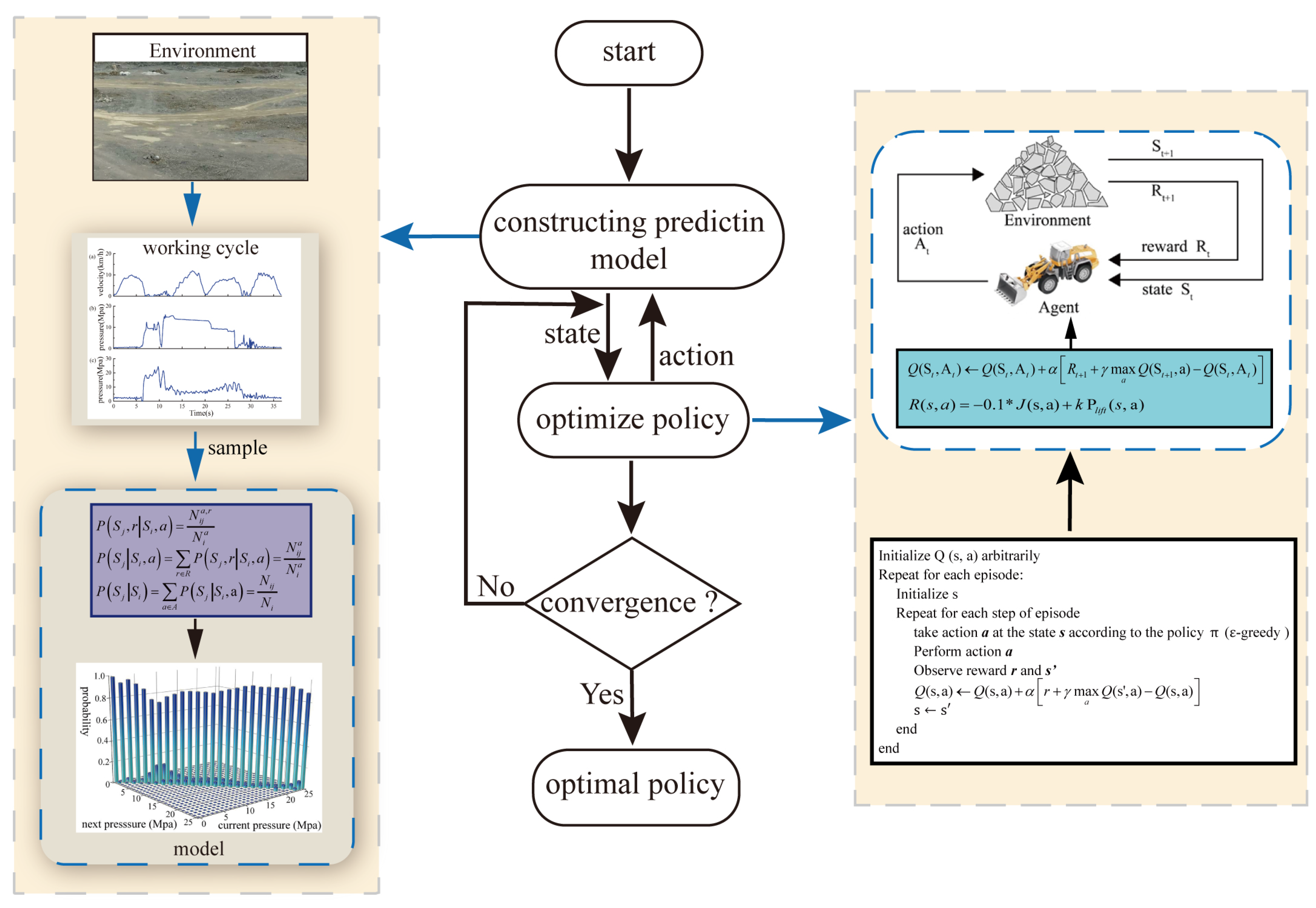
In this paper, a data-driven RL-based approach is proposed for automatic bucket-filling of wheel loaders to achieve low costs and adapt to changing conditions. The Q-learning algorithm can learn from different conditions and is used to learn the optimal action in different states by maximizing the expected sum of rewards. Aiming to achieve low costs, an indirect RL is employed. Indirect RL requires a virtual environment constructed from data or the known knowledge, and the agent learns from interacting with the virtual environment instead of the real environment. Direct RL needs to interact with the real environment, and the agent of direct RL learns from interacting with the real environment. Compared to direct RL, indirect RL can more efficiently take advantage of samples by planning [6]. In addition, the parameters of Q-learning in source tasks are partially transferred to the Q-learning of target tasks to demonstrate the transfer learning capability of the proposed approach. Considering the nonlinearity and complexity of interactions between the bucket and pile [7], the data obtained from field tests are utilized to build a nonlinear, non-parametric statistical model for predicting the state of the loader bucket in the bucket-filling process. The prediction model is used to train the Q-learning algorithm to validate the proposed algorithm.

The main contributions of this paper are summarized as follows:

(1)

A data-based prediction model for the wheel loader is developed.

(2)

A general automatic bucket-filling algorithm based on Q-learning is presented and the transfer ability of the algorithm is demonstrated. The proposed automatic bucket-filling algorithm does not require a dynamic model and can adapt for different changing conditions with low costs.

(3)

The performance of the automatic bucket-filling algorithm and expert operators on loading two different materials is compared.

The rest of this paper is summarized below. Section 2 presents the related existing research. Section 3 states the problem and develops the prediction model. Section 4 details the experimental setup and data processing. Section 5 explains the automatic bucket-filling algorithm based on Q-learning and presents the state and reward. Section 6 discusses the experimental results and evaluates the performance of our model by comparing it with real operators. Lastly, the conclusions are drawn in Section 7.

2. Related Works

Numerous researchers have attempted to use different methods to achieve automatic bucket-filling. These studies can be summarized into the following three categories, which are: (1) physical model-based, (2) neural networks-based, and (3) reinforcement learning (RL)-based. This section will review related works in these three aspects, respectively.

Most relevant research attempted to realize automatic bucket-filling via physical-model-based control [8]. Meng et al. [9] applied Coulomb’s passive earth pressure theory to establish a model of bucket force during the scooping process for load-haul-dump machines. The purpose of developing the model was to calculate energy consumption, and the trajectory was determined through optimizing the minimum energy consumption in theory. Shen and Frank [10,11] used the dynamic programming algorithm to solve the optimal control of variable trajectories based on the model of construction machinery. The control results are compared to an extensive empirical measurement done on a wheel loader. The results show that the fuel efficiency is higher compared to the fuel efficiency measured among real operators. These works require accurate machine models, so they are prone to collapse under conditions of modeling errors, wear, and change. An accurate model of the bucket-pile interaction is difficult to build because the working condition is unpredictable, and the interaction forces between the bucket and material are uncertain and changing. When the machine and materials change, the model needs to be rebuilt. Therefore, the model-based approach is not a generic automatic bucket-filling solution for various the bucket-pile environments.

In recent years, non-physical-model-based approaches [12] have been employed in the autonomous excavation of loaders and excavators. With the development of artificial intelligence, neural networks have been used in non-model-based approaches. A time-delayed neural network trained on expert operator data has been applied to execute the bucket-filling task automatically [13]. The results show that time-delayed neural network (TDNN) architecture with input data obtained from the wheel loader successfully performs the bucket-filling operation after an initial period (100 examples) of imitation learning from an expert operator. The TDNN algorithm is used to compare with the expert operator and performs slightly worse than the expert operator with 26% longer bucket-filling time. Park et al. [14] utilized an Echo-State Networks-based online learning technique to control the position of hydraulic excavators and compensate for the dynamics changes of the excavators over time. Neural network-based approaches do not require any machine and material models. However, these approaches require a large amount of labeled data obtained from expert operators for training, which is too costly.

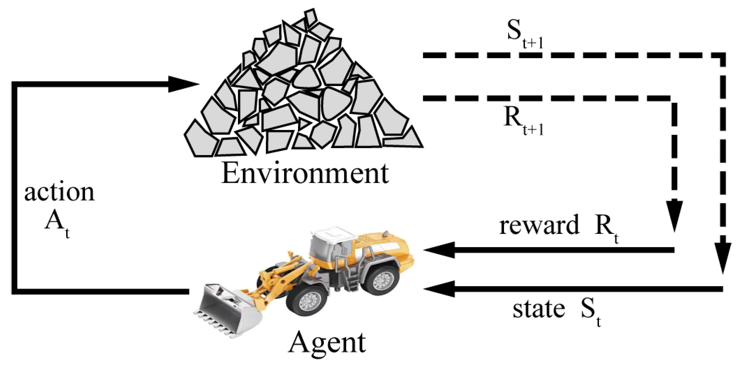
Reinforcement learning (RL) is capable of learning effectively through interaction with complex environments without labeled data. The learning procedure of RL includes perceiving the environmental state, taking related actions to influence the environment, and evaluating an action by the reward from the environment [15]. Reinforcement learning not only achieved surprising performance in GO [16] and Atari games [17], but has also been widely used for autonomous driving [18] and energy management [19]. The application of RL in construction machinery automation is mainly based on real-time interaction with the real or simulation environment. Hodel et al. [20] applied RL-based simulation methods to control the excavator to perform the bucket-leveling task. Kurinov et al. [21] investigated the application of an RL algorithm for excavator automation. In the proposed system, the agent of the excavator can learn a policy by interacting with the simulated model. Because simulation models are not derived from the real world, RL-based simulation cannot learn features of the real world well. Dadhich et al. [5] used RL to achieve the automatic bucket-filling of wheel loaders through real-time interaction with the real environment. However, interacting with the real environment to train the RL algorithm is costly and time-consuming.

3. Background and Modeling

3.1. Working Cycle

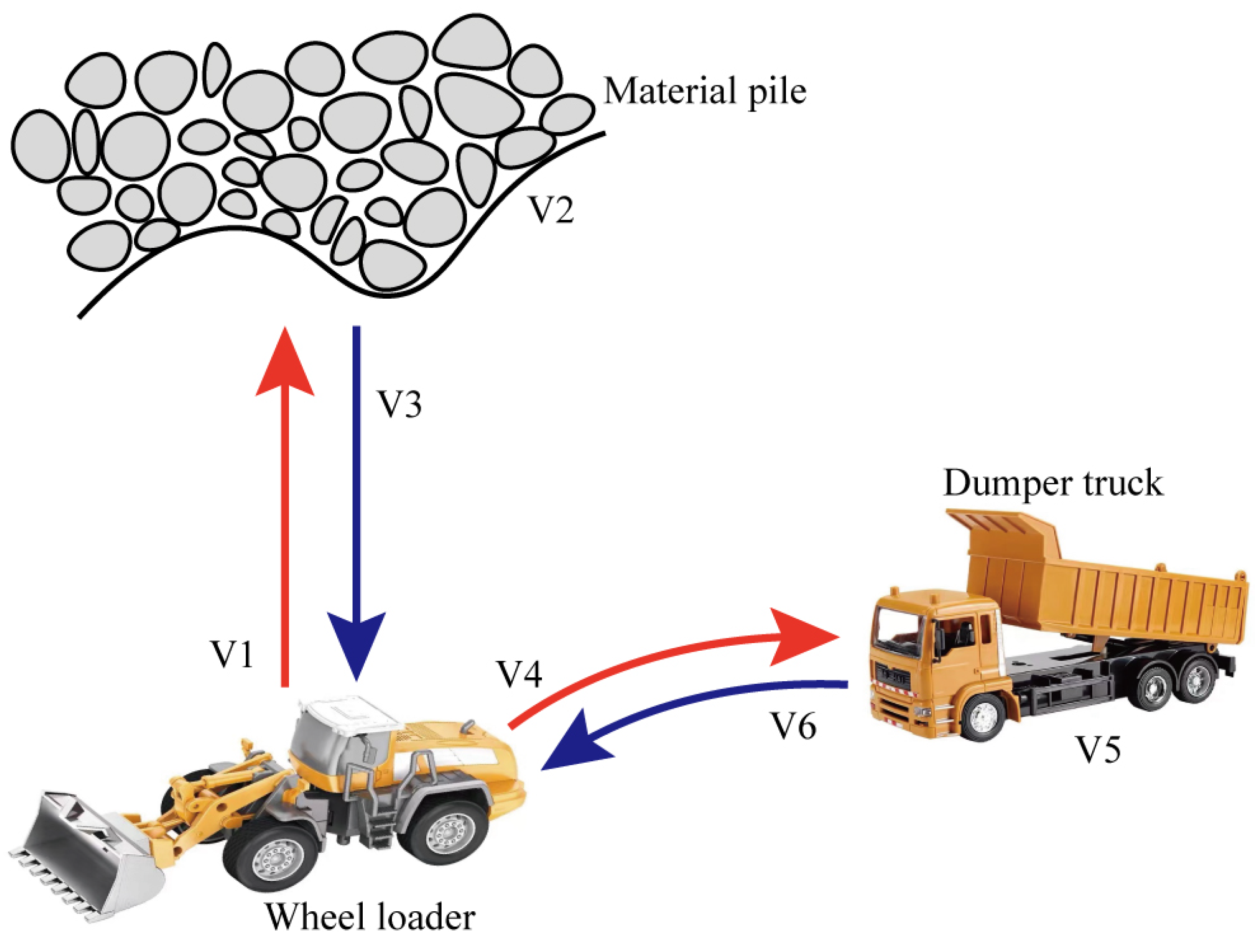
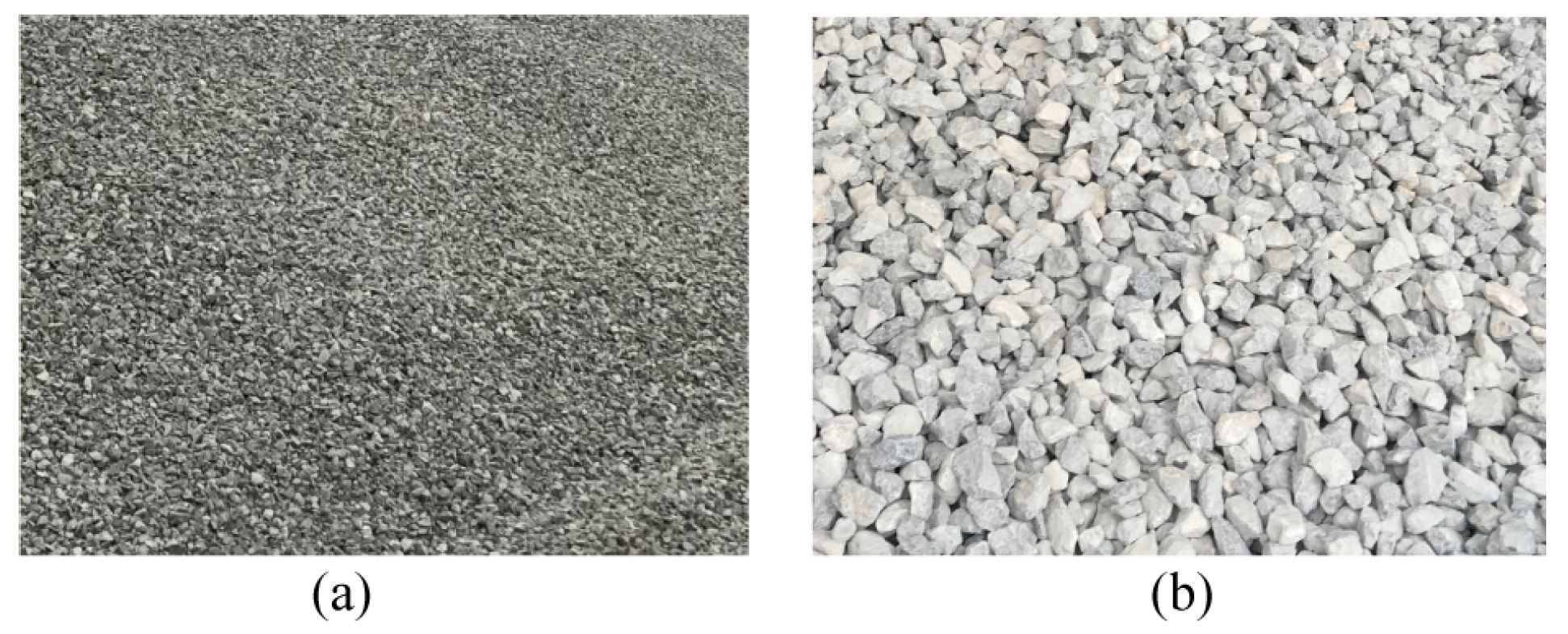
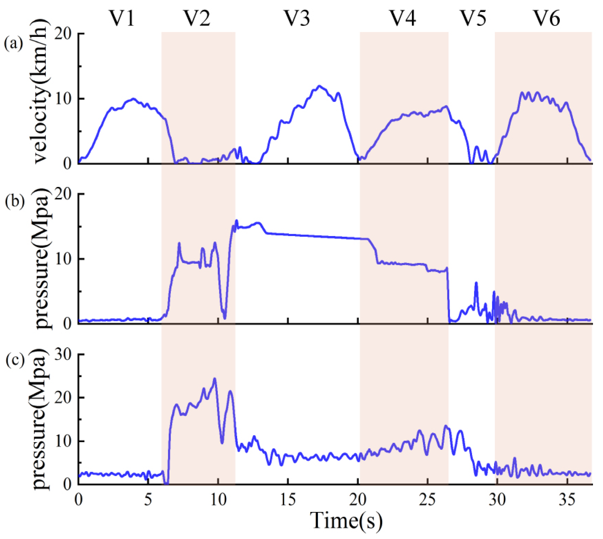
Wheel loaders are used to remove material (sand, gravel, etc.) from one site to another or an adjacent load receiver (dump truck, conveyor belt, etc.). Although there are many repetitive operation modes in the working process of wheel loaders, the different working cycles increase the complexity of data analysis. For wheel loaders, the representative short loading cycle, sometimes also dubbed the V-cycle, is adopted in this experiment, as illustrated in Figure 1. The single V-cycle is divided into six phases, namely, V1 forward with no load (start and approach the pile), V2 bucket-filling (penetrates the pile and load), V3 backward with full load (Retract from the pile), V4 forward and hoisting (approach to the dumper), V5 dumping, and V6 backward with no load (Retract from the dumper), as shown in

Table 1. Basic parameters of the experimental wheel loader.

Parameters	Value	Units
Length	6600	mm
width	2750	mm
Height	3470	mm
Maximum traction	175	kN
rated power	162	kW
Rated load	5	t

. This article only focuses on the automation of the bucket-filling process (V2), which highly affected the overall energy efficiency and productivity of a complete V-cycle. The bucket-filling process (V2) accounts for 35–40% of the total fuel consumption per cycle [22]. In the bucket-filling process, the operator needs to modulate three actions simultaneously: a forward action (throttle), an upward action (lift), and a rotating action of the bucket (tilt) to obtain a large bucket weight.

3.2. Problem Statement

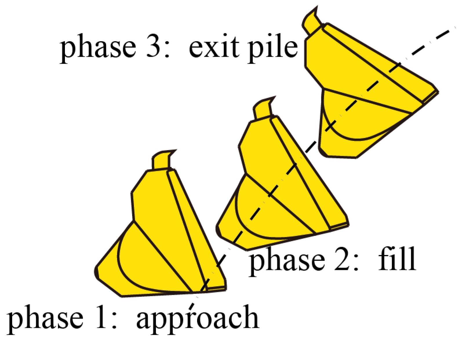
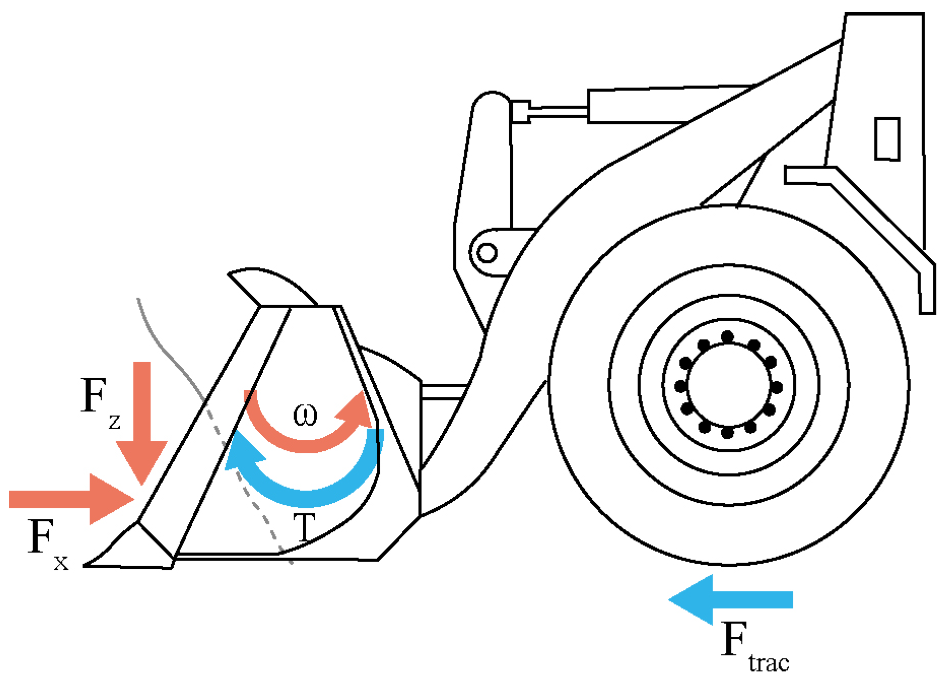
The working process of scooping can be split into three stages: approach, fill, and exit the pile, as shown in Figure 2. In the first stage, wheel loaders move towards the pile of earth and the bucket penetrates the soil. In the second stage, the operator simultaneously adjusts the lift, tilt, and throttle to navigate the bucket tip through the earth pile and load as much material as possible within a short period. The throttle controls the engine speed, while the lift and tilt levers command valves in the hydraulics system that ultimately control the motion of the linkage’s lift and tilt cylinder, respectively. In the third phase, the bucket is tilted until the breakout is involved and the bucket exits the pile. The scoop phase is treated as a stochastic process where the input is the wheel loader state, and the output is the action. The goal is to find a policy using RL that maps the wheel loader state to action.

3.3. Prediction Model

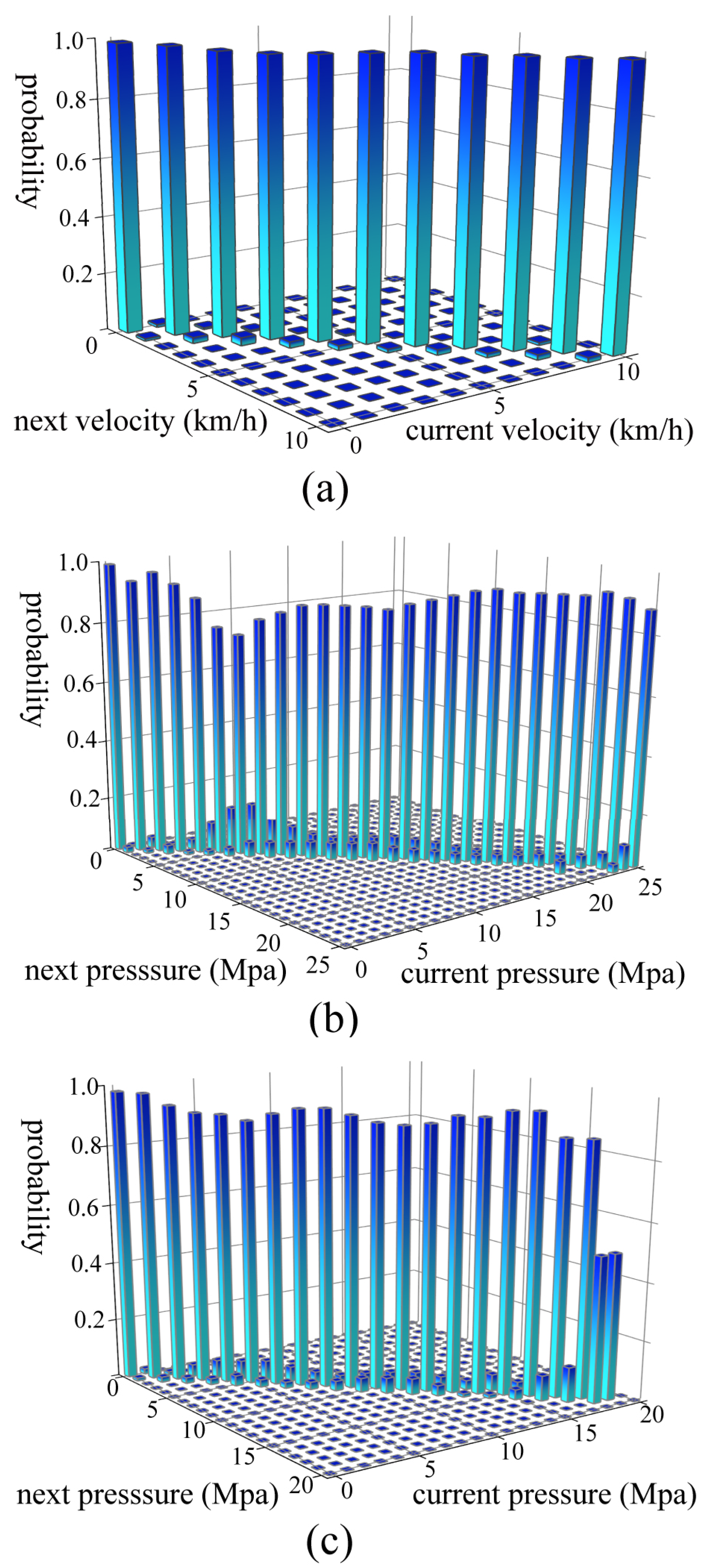
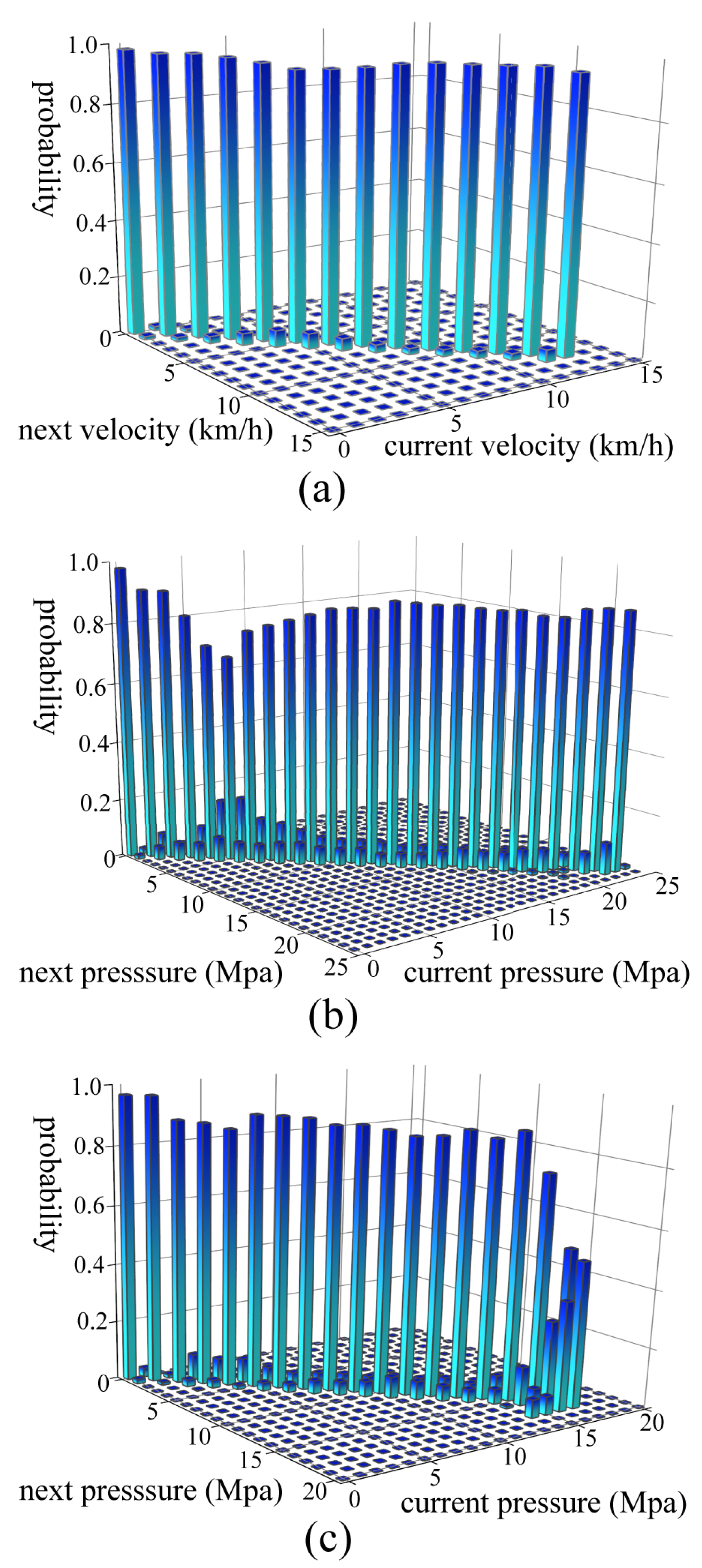
The Markov property is a prerequisite for reinforcement learning. In the actual operation process, the operator mainly executes the next actions according to the current state of the loader. Thus, the wheel loader state of the scooping process at the next moment is considered not to be related to the past, but to the current state, which satisfies the Markov property. Therefore, the interaction between the wheel loader bucket and the continuously changing pile can be modeled as a Finite Markov decision process (FMDP) which is expressed by a quadruple $F\left(S,A,P,R\right)$, consisting of the set of possible states S, the set of available actions A, the transition probability P, and the reward R. The state $s\in S$ includes the velocity, the tilt cylinder pressure, and the lift cylinder pressure. The actions consist of lift, tilt, and throttle commands which are all discrete. The ranges of lift, tilt, and throttle commands are from 0 to 160, 0 to 230, and 0 to 100, respectively. Besides, as the pile’s shape and loaded material vary randomly, the change of the pile is considered as a stochastic process, which also satisfies the Markov property. Therefore, the problem of automatic bucket-filling for wheel loaders is considered as a finite Markov decision process (FMDP).

To achieve indirect RL, a prediction model needs to be constructed to predict the wheel loader state at the next moment according to the current state and action during the scooping phase. In this paper, changes in the wheel loader state are regarded as a series of discrete dynamic stochastic events and described with a Markov chain. The transition probability can be expressed as:

$$P\left(S_j|S_i\right)=\frac{N_{i,j}}{N_i},$$

(1)

where $N_{ij}$ is the number of times the wheel loader state transits from $S_i$ to $S_j$, and $N_i$ is the total number of times the wheel loader state transits from $S_i$ to all possible states.

The prediction model of the wheel loader state can be expressed as:

$$P\left(S_j,r|S_i,a\right)=\frac{N_{i,j}^{a,r}}{N_i^a},$$

(2)

where $P\left(S_j,r|S_i,a\right)$ denotes the probability of state transits from $S_i$ to $S_j$ and to get a reward r when action a is taken in state $S_i$, $N_i^a$ is the total number of times the wheel loader state transits from $S_i$ to all possible states when action a is taken, and $N_{i,j}^{a,r}$ is the total number of times the wheel loader state transits from $S_i$ to $S_j$ when action a is taken and gets the reward r.

Python is used to construct the prediction model. We read the experimental data in sequence. The current state $S_t$ and action a are stored as a key of the Python dictionary, and the value corresponding to the key is another dictionary whose keys are the next state $S_{t+1}$ and reward r, and values are $P\left(S_{t+1},r|S_t,a\right)$. According to the current state $S_t$ and action a, the next state $S_{t+1}$ and reward r are selected randomly with probability.

The prediction model can approximate the real working environment, as it is built using the real data obtained from tests. Besides, the prediction model not only covers the working information of wheel loaders, but also reflects the environmental effect. The sampling frequency is important because the complexity of the model can be controlled by adjusting the sampling frequency. The high sampling frequency will increase the complexity of the model and the computation load, while the low sampling frequency might cause model distortion.

4. Experiment and Sampling

4.1. Experimental Setup

The experimental wheel loader is shown in Figure 3. it is equipped with pressure sensors, displacement sensors, and GPS. The Liugong ZL50CN wheel loader is taken as the experiment machine. The basic parameters of the wheel loader are listed in Table 1. In order to verify whether the proposed automatic bucket-filling algorithm can converge to the optimal strategy on the data model based on different piles, we collected data from two types of piles, which are shown in Figure 4. It has been proven that the Q-learning algorithm with lookup tables are guaranteed to converge to the optimal solution. Small coarse gravel (SCG) mainly contains particles up to 25 mm, while medium coarse gravel (MCG) mainly contains particles up to 100 mm.

4.2. Data Acquisition and Processing

According to the working characteristics of wheel loaders in a working cycle, the V-cycle is divided by extracting the working condition features of the actuator and walking device, including suspension, axle housing, tires, and rims. The mapping between the collected data and the working state is realized by dividing the V-cycle, as shown in Figure 5. The data in the scooping phase were selected to develop the prediction model. There was no benchmark dataset. For different piles, we collected 51 sets of data to build prediction models. The sampling frequency was 200 HZ. Due to the high dimension of the state vector, it is difficult to present the complete prediction model in a figure. Therefore, transition probability maps for the individual elements of the state vector are drawn and transition probability maps of different materials are similar, as shown in Figure 6 and Figure 7. Figure 6 and Figure 7 based on Equation (1) reflect the virtual environment built from real data and the changing trend of states corresponding to different piles at the next moment.

5. Automatic Bucket-Filling Algorithm

5.1. Automatic Bucket-Filling Algorithm Based on Q-Learning

Reinforcement learning is learning what to do—how to map situations to actions—so as to maximize the expected discounted long-term reward. The two most important distinguishing features of reinforcement learning are trial-and-error search and delayed reward. The learner and decision-maker are called the agent. At each time-step, the agent takes action a according to the current environmental state $S_t$ and the policy $\pi$ which is a mapping from perceived states to actions. Therefore, as a consequence of action, the environmental state transits from $S_t$ to $S_{t+1}$ and the agent gets a reward r. The agent and environment generate the trajectories ($S_1$; $A_1$; $R_1$), ($S_2$; $A_2$; $R_2$), …, ($S_T$; $A_T$; $R_T$) [23], until an episode is over. The basic architecture of RL is shown in Figure 8.

Q-learning is a widely used RL algorithm. Similar to other classical RL methods, the goal of Q-learning is to obtain an optimal policy that maximizes the long-term reward. In the Q-learning algorithm, the agent receives the reward and updates the Q-function corresponding to the action-state. The Q-function represents the expected estimated accumulated reward for the action-state pair under a policy. For example, $Q(S_t,A_t)$ is denoted as the expected long-term reward starting from state $S_t$, taking action $A_t$. By continuous exploitation and exploration, the agent will eventually obtain the optimal Q-function $\left(Q_{*}\right)$ which determines the action selection policy. The optimal policy ${\pi }^{*}\left(S_t\right)$ can be calculated by the following equation:

$${\pi }^{*}\left(S_t\right)=arg\underset{a\in A}{max}{Q}_{*}\left(S_t,A\right),$$

(3)

where $Q_{*}(S_t,A)$ is the maximum Q-function over all policies. The optimal policy ${\pi }^{*}\left(S_t\right)$ is to select the action that maximizes the $Q_{*}(S_t,A)$.

The Bellman equation of the optimal Q-function $\left(Q_{*}\right)$ is:

$$Q_{*}\left(S_t,A_t\right)=\sum _{S_{t+1},r}P\left(S_{t+1},r|S_t,A_t\right)\left[r+\gamma \underset{A_{t+1}}{max}{Q}_{*}\left(S_{t+1},A_{t+1}\right)\right],$$

(4)

where $\gamma \in \left[0,1\right]$ is the discount factor that determines the present value of future rewards.

The Q-learning algorithm is designed by the Bellman equation and contraction mapping theorem. Q-learning is defined by

$$Q\left(S_t,A_t\right)\leftarrow Q\left(S_t,A_t\right)+\alpha \left[R_{t+1}+\gamma \underset{a}{max}Q\left(S_{t+1},a\right)-Q\left(S_{t+1},A_t\right)\right],$$

(5)

where $\alpha \in \left[0,1\right]$ is the learning rate which reflects the influence of the new experience on the current estimation $Q(S_t,A)$.

Q-learning starts with an initial $Q(S_1,A_1)$ for each state-action pair. At each time-step, the agent performs an action based on a commonly used exploration method $\epsilon$ greedy strategy that selects the greedy action with probability $1-\epsilon$, but every once in a while, it selects randomly from all the actions with equal probability $\epsilon$ independently of the action-value estimates. Each time an action a is taken in state s, then the reward r is fed back from the environment and the next state $s^{,}$ is observed, thus the Q-value is updated with a combination of its current value and the Temporal-Difference Error (TDE)(date-drive). The pseudo-code of the Q-learning algorithm is shown in Figure 9. The code can be found in supplementary materials.

In this study, Q-learning based on a prediction model was used to optimize the choice of actions. The Q-learning architecture in automatic bucket-filling is illustrated in Figure 10. By using the real data, the environmental characteristics can be abstracted into the prediction model. Q-learning is trained on the prediction model until the algorithm converges. By interacting with the prediction model built from the collected real data, the agent is able to learn the working characteristics of wheel loaders and the optimal strategy. Based on the prediction model, the Q-function can be updated via the learning process of the agent. To investigate the transfer ability of the proposed algorithm, the automatic bucket-filling algorithm is first trained on a bucket-pile interaction model and then the Q-function learned from the previous model is transferred to the target task to enhance the learning efficiency and the learning rate on the bucket-pile interaction model of the target task.

5.2. State and Reward Representation

The appropriate state and reward function should be set to optimize action selection. The state needs to be able to reflect the characteristics of the environment when the agent interacts with the environment and the dimensionality should not be too high to avoid the curse of dimensionality. Lift force is the most important feature affecting the lift and tilt commands [13] and lift force is related to the lift cylinder pressure. Besides, the velocity of wheel loaders is of significance to the choice of throttle command. The tilt cylinder pressure can be used as a redundant feature. Thus, in this study, we defined the state using a three-dimensional vector consisting of velocity, tilt cylinder pressure, and lift cylinder pressure, which are expressed as:

$$S=\left\{s=\left[V_{loader},P_{lift},P_{tilt}\right]\right\},$$

(6)

where $V_{loader}$ is the velocity of wheel loaders, $P_{lift}$ is the lift cylinder pressure, and $P_{tilt}$ is the tilt cylinder pressure.

It can be seen from Figure 11 that the bucket-soil interaction force mainly depends on the amount of loaded soil. Therefore, the bucket-soil interaction force can directly translate into the amount of loaded soil and is important for the bucket-filling of wheel loaders. In order to encourage the loader to improve the bucket digging force and fuel economy during the training process, the reward function should be composed of the negative value of fuel consumption and the bucket-pile interaction force. Because the bucket-soil interaction force is difficult to measure directly and has a positive correlation with lift cylinder pressure, we use the lift cylinder pressure as a part of the reward function to represent digging force. The bigger bucket digging force demands increased fuel consumption. Therefore, a trade-off is necessary between the fuel consumption and bucket digging force. The reward function is expressed as follows:

$$R\left(s,a\right)=-0.1\ast J\left(s,a\right)+k{P}_{lift}\left(s,a\right),$$

(7)

where $J(s,a)$ is the fuel consumption from the current state s to the next state $s^{\prime }$ when the agent takes action a, $P_{lift}(s,a)$ is the lift cylinder pressure of next state $s^{\prime }$, and k is a constant to control the priority of the fuel economy and bucket weight and $k=0.2$.

6. Results and Discussions

In this section, the proposed automatic bucket-filling algorithm is utilized to learn the policy on prediction models and present the results. We choose 0.15 as the learning rate of Q-learning, $\epsilon$ in the $\epsilon$ greedy policy is 0.1, and the discount factor $\gamma$ = 0.15.

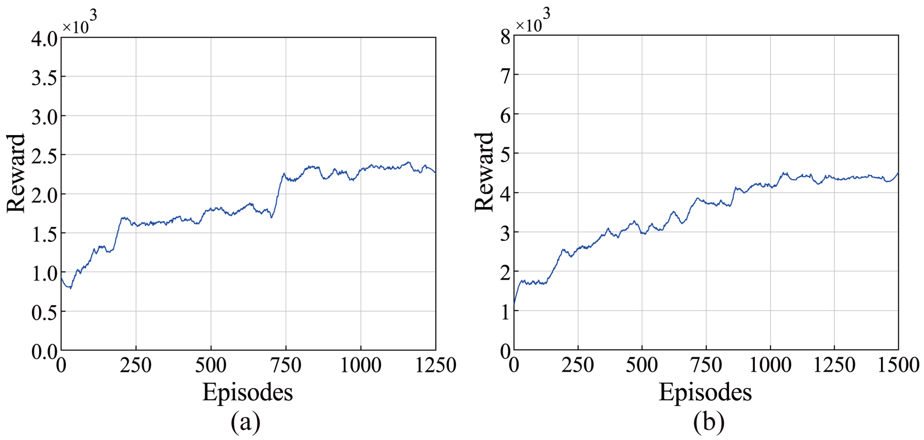
Wheel loaders have a complicated working environment and are used to transport different materials. In order to verify the convergence of the algorithm on the diverse environment, the reward curves based on different prediction models are depicted in Figure 12. It can be observed that the proposed automatic bucket-filling algorithm can converge to the optimal policy that maximizes reward, indicating that the agent was learning the policy correctly under different prediction models. This shows that the proposed algorithm can be adapted to different bucket-pile models, thus dealing with the complex and changing working environment of wheel loaders in the absence of a complex dynamic model.

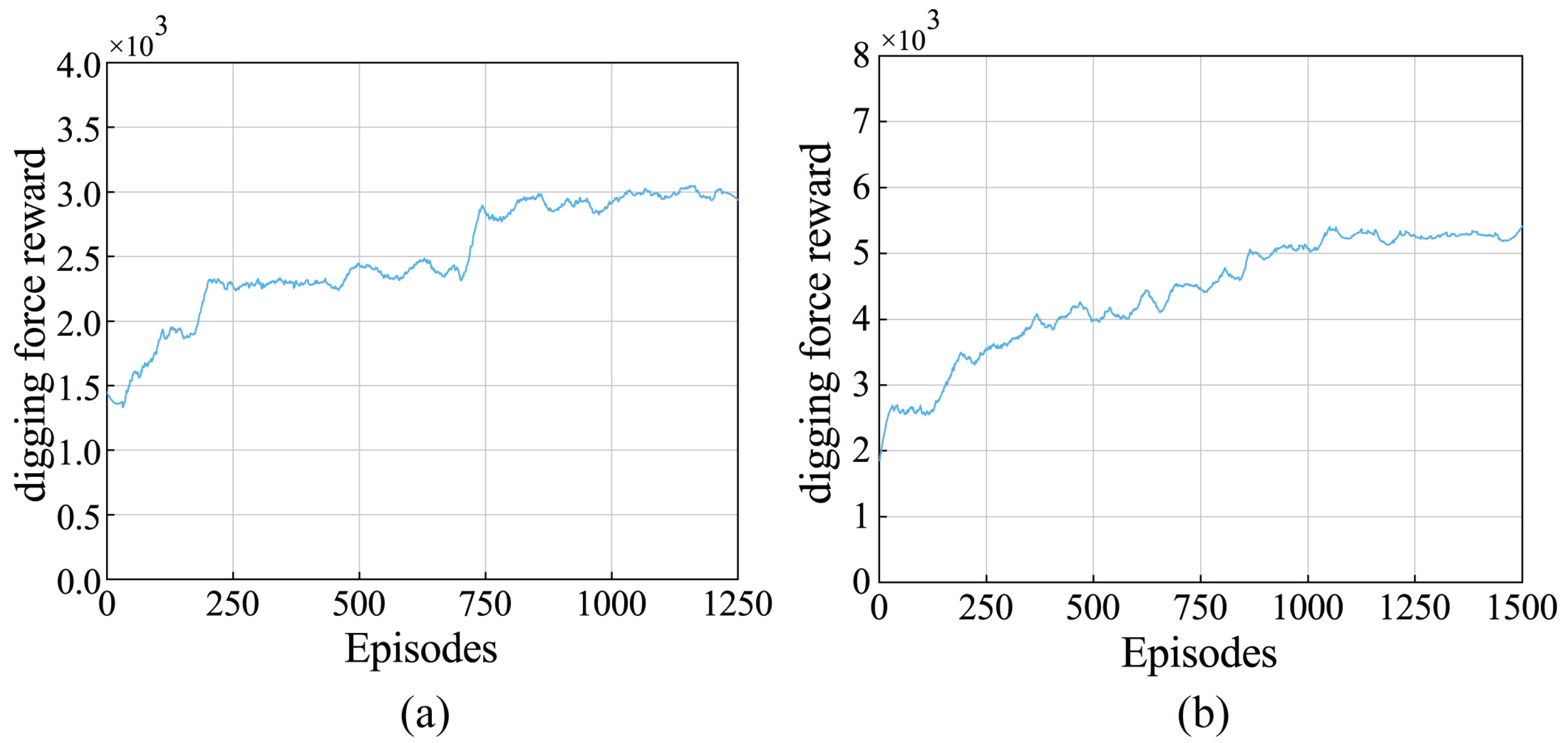
The digging force reward per episode is obtained by accumulating the lift cylinder pressure of each step and is used to approximate the change of digging force. As can be seen from Figure 13, compared with the algorithm interacting with the small coarse gravel model, the algorithm interacting with the medium coarse gravel model can converge to a smaller value of digging force reward. A larger digging force usually leads to higher fuel consumption. Thus, loading small coarse gravel has higher fuel consumption compared to medium coarse gravel on this data-based prediction model, as shown in Figure 14. This finding suggests that the prediction model can truly reflect the interaction between the bucket and the material to a certain extent.

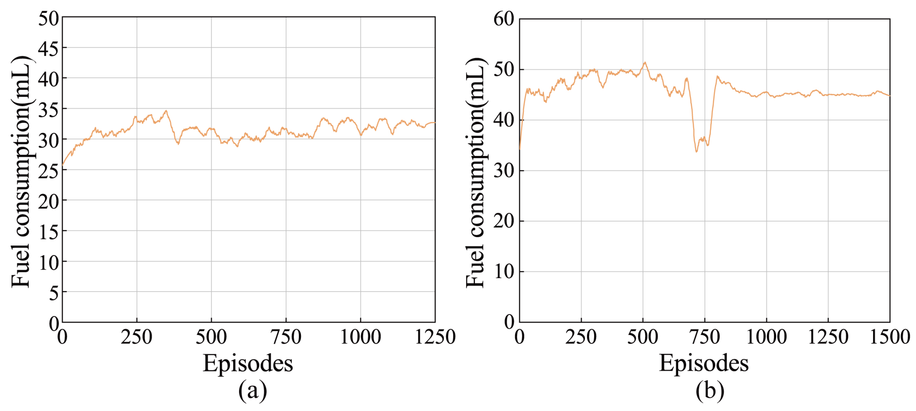
The results of fuel consumption of the agent in different models are shown in Figure 14. The data used to build the model come from the real environment. The wheel loader operated by a human operator is the same as the wheel loader used to obtain the data. In addition, the working environment of the wheel loader is also the same. Therefore, the agent we trained has the same operating object and operating environment as the human operator. A comparison with humans is used as a generally accepted method of machine learning algorithm testing [11,13]. Physical-model-based methods require a physical model. However, the diversity between the physical model and the wheel loader used to obtain the data is great. In addition, the environment constructed for the physical model is also very different from the environment constructed in the article. Therefore, physical-model-based methods and the method proposed in this article have different operating objects and environments. In addition, deep learning-based methods mainly predict actions based on previous actions and states. As deep learning-based methods mainly solve the prediction problem, root mean square error (RMSE) is used as the evaluation indicator, which is different from our paper. Therefore, the fuel consumption measured by the human operator is used to compare with the fuel consumption of the agent.

Table 2. The comparison of fuel consumption.

Pile	Average Fuel Consumption of Recorded Bucket-Filling Phase (mL)	Variance	Convergence Value (mL)	Improvement (%)
medium coarse gravel	36.2	61.6	33.3	8.0
small coarse grave	51.0	42.8	45.6	10.6

shows the average fuel consumption of loading different piles and the variance of fuel consumption in the recorded bucket-filling phase. In Figure 14b, there is a relatively stable convergence, while in Figure 14a, the curve fluctuates violently. A possible explanation for this is that the prediction model built by data with higher variance is more complex and variable. Therefore, the agent will encounter more situations in each episode, resulting in the oscillation of the convergence curve. In addition to this, the convergence values of fuel consumption of agents on medium coarse gravel model and small coarse gravel model are around 33.3 mL and 45.6 mL, respectively, and improve by 8.0% and 10.6% compared to the average fuel consumption measured by real operators because Q-learning can learn the optimal action in different states.

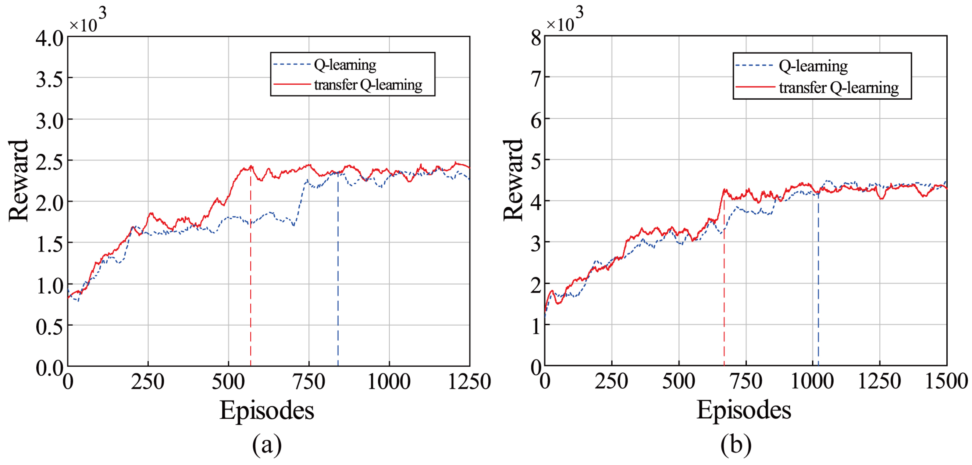
The transfer learning ability can help the algorithm to improve the learning performance on new bucket-filling tasks, thereby saving training costs. In this paper, transfer Q-learning refers to the Q-learning that has been trained in other tasks and learned relevant knowledge.

Figure 15 shows the convergence curve of rewards for Q-learning and transfer Q-learning in the different bucket-pile interaction models. In Figure 15a, Q-learning is only trained on the MCG-pile model, and transfer Q-learning is first trained on the SCG-pile model and then trained on the MCG-pile model. In Figure 15b, Q-learning is only trained on the SCG-pile model, and transfer Q-learning is first trained on the MCG-pile model and then trained on the SCG-pile model. The convergence rate (learning rate efficient) of Q-learning and transfer Q-learning in two bucket-pile interaction models are compared, as presented in

Table 3. The comparison of Q-learning and transfer Q-learning on convergence speed.

Pile	Convergence Episode of Q-Learning	Convergence Episode of Transfer Q-Learning	Improvement (%)
medium coarse gravel	825	575	30.3
small coarse grave	1025	675	34.1

. Using Q-learning as the benchmark, the convergence speed of transfer Q-learning in the medium coarse gravel and small coarse gravel model is improved by 30.3% and 34.1%, respectively. This means that the proposed algorithm has a good transfer learning capability. This improvement can be ascribed to the fact that Q-learning stores the learned knowledge in the Q-function and the transfer Q-learning transfers the Q-function learned from the source task to the Q-function of the target task. Therefore, the agent no longer needs to learn the basic action characteristics in the bucket-filling phase.

When the two piles have similar characteristics, such as in category and shape, transfer Q-learning might have better performance in the new bucket-filling task due to the similarity of the optimal Q-function in two tasks [24]. Finally, the amount of data used to build the interaction model also has an impact on the performance of transfer Q-learning on the prediction model. The more data there is, the more states and actions the developed prediction model contains. Therefore, different prediction models have more identical states and actions, and the Q-function of the target task can learn more knowledge from the Q-function of the source task. However, the transfer learning method potentially does not work or even harm the new tasks [25] when the piles or environment are greatly different.

7. Conclusions

This paper investigated the automatic bucket-filling algorithm based on RL for wheel loaders, and the algorithm was tested. The data-driven prediction model was established using previously obtained excavation data of two piles. The transfer Q-learning-based automatic bucket-filling algorithm was proposed, and the algorithm was trained on the prediction model. The results of training show that the proposed algorithm has good performance of adaptability and convergence even without parameters of wheel loaders. Moreover, the proposed algorithm has good performance in fuel consumption, with 8.0% and 10.6% reduction compared to the average fuel consumption measured by real operators on two piles. Transfer learning is used to transfer the parameter of Q-learning in the source task to the target task. The results show the promising performance of the proposed method on an automatic bucket-filling task. The proposed data-driven RL-based approach in this paper has generality, which means that this approach can be applied to different machine-pile environments. Furthermore, compared to most previous solutions for the automation of bucket-filling, the approach proposed in this paper does not require a dynamic model and has the advantages of no direct interaction with the real environment and transfer ability. In future research, the method proposed in this paper will be applied to the real wheel loaders and compared with other methods to further enhance the performance of the reinforcement-learning-based automatic bucket-filling algorithm.