A Robot Dynamic Target Grasping Method Based on Affine Group Improved Gaussian Resampling Particle Filter

Abstract

Tracking and grasping a moving target is currently a challenging topic in the field of robotics. The current visual servo grasping method is still inadequate, as the real-time performance and robustness of target tracking both need to be improved. A target tracking method is proposed based on improved geometric particle filtering (IGPF). Following the geometric particle filtering (GPF) tracking framework, affine groups are proposed as state particles. Resampling is improved by incorporating an improved conventional Gaussian resampling algorithm. It addresses the problem of particle diversity loss and improves tracking performance. Additionally, the OTB2015 dataset and typical evaluation indicators in target tracking are adopted. Comparative experiments are performed using PF, GPF and the proposed IGPF algorithm. A dynamic target tracking and grasping method for the robot is proposed. It combines an improved Gaussian resampling particle filter algorithm based on affine groups and the positional visual servo control of the robot. Finally, the robot conducts simulation and experiments on capturing dynamic targets in the simulation environment and actual environment. It verifies the effectiveness of the method proposed in this paper.

1. Introduction

In recent years, with the development of robot technology, robot vision has become the forerunner of machine vision, and vision has also become one of the most important sensing technologies for robots [1,2]. Target grasping is one of the most typical applications in robotics. The combination of machine vision and robot control provides a feasible solution for tracking and grasping dynamic targets [3,4].

For multi-target object grabbing on low-speed conveyor belts, Zhang et al. [5] extracted local features (via SIFT) from the visual image sequences of a target and mapped the key points of each image to a unified dimensional histogram vector. However, SVM classifiers require much offline training to achieve good results, and a large number of SIFT feature points of sample images need to be extracted during training. Hu et al. [6] considered an image block as a second-order tensor and constructed a discriminant embedding space. They mapped the original tensor sample to the tensor-based graph embedding space. The semi-supervised strategy was applied to visual tracking.

Some researchers adopted the strategy of block modeling and tracking. For detection and tracking in the case of target occlusion, Zhang et al. [7] followed the fragment modeling idea in [8], fused the idea in [9] and applied a horizontal and vertical axis slicing method to modeling. It solves the tracking problem for full occlusion. However, for background clutter in complex environments, there is still a problem with its tracking performance. Sun et al. [10] proposed a block modeling method based on color distribution. It improved the adaptability to complex situations such as illumination variation.

Other researchers focused on multi-dimensional moving target tracking. Song et al. [11] proposed a three-dimensional attitude tracking method that combined “1-Step GA” and manual feedback compensation. It was different from the optimized tracking method based on Taylor expansion and did not fall into problematic local minima. Lin et al. [12] used two CCDs as stereo vision sources to separate targets from paired images. They calculated the centroid coordinates of each target image and determined the space position of targets. The Lagrange interpolation formula and linear function were used to simulate the trajectory of the ball, and the catching position was predicted. Salehian et al. [13] used the OptiTrack system to capture the target ball and first learned the trajectory of the parabola via a machine learning algorithm. The computer can quickly predict the trajectory of the target when grasping. It indirectly achieves recognition and tracking through the target ball on the target, which has certain limitations. Issac et al. [14] studied the model-based three-dimensional tracking problem with dense depth images as input. They used the Gaussian filter robustification method to address the problem of the thick-tail measurement noise of the depth sensor. Experiments indicated that the performance was better than that of the standard Gaussian filter and particle filtering (PF) tracking methods.

Many researchers used the method of matching and probabilistic prediction and tracking in their research for complex environments with limited viewing angles. Li et al. [15] used the distributed learning ability of a generative adversarial network (GAN) to propose a general multi-agent probabilistic prediction and tracking framework. The framework considered the interaction between multiple entities and treated all entities as a whole. However, as GAN training was very difficult, the applicability of the algorithm was reduced. Solaimanpour et al. [16] proposed a new hierarchical hidden Markov model and an online algorithm for learning the parameters from observed data collected during operation. A nested particle filter used robot observations to measure the weight of nested particles while self-locating and tracking another robot. Xu et al. [17] combined Kalman filtering and PF to propose a varying particle-filtering method for targets with a linear and nonlinear motion. It increased the importance of sampling, the fusion of the likelihood function, the prior distribution, and the accuracy of the PF algorithm. Chen et al. [18] built a vision-guided grasping system, which adopted the edge particle filter algorithm to obtain parameters such as target position, speed, and acceleration. It realized the tracking of plane moving objects by a robotic arm. However, the system does not use claws for grasping, and the pose is not considered. Hussain et al. [19] used geometric particle filtering (GPF) based on reflection groups to realize three-dimensional space target tracking. This method only used depth information and did not rely on texture features. Zhang et al. [20] proposed a multi-task related particle filter. Compared with the conventional particle filter, this filter maintained multiple modes in the posterior density, reducing the computational cost. Kwon et al. [21,22] proposed GPF using 2D affine transformation groups as particles. It had excellent performance for image tracking with a given target template. However, simple resampling resulted in decreased particle diversity.

Some researchers carried out research on interception grabbing of unknown objects. Denis Stogl et al. [23] proposed a method for tracking, reconstructing, and grasping unknown objects from a moving conveyor belt using external depth sensors and industrial robots. The method includes an algorithm for estimating the position, speed and shape of the object. It includes an algorithm of the conveyor path and an algorithm for calculating the interception trajectory of the robot. Jie Huang et al. [24] introduced the attraction vector to describe the relative posture between the object and the end effector to achieve tracking in a dynamic environment. Zhou Zhao et al. [25] used an improved spatio-temporal context tracking algorithm to track the moving target and calculated the position of the gripper in the base coordinate system. In order to complete the grasping task, a linear prediction method was used to predict the moving object in a three-dimensional space. Takuya Omi et al. [26] used the same hand to detect the grasping and release of objects. The correspondence between the objects is observed before and after the object is occluded. It is used for object tracking in the living space and the body segmentation of each object. It is also achieved by detecting its grasp and release. Hongxiang Yu et al. [27] introduced the Neural Acceleration Estimator, which estimates the changing acceleration by observing a small part of the previous deflection trajectory of the flying object. It uses the end-to-end training of the differential filter to measure the error. The experimental results show that it also has good generalization for unknown objects.

Existing Limits and Our Contributions

Based on the above research, the method based on matching and probability prediction has certain limitations. The OptiTrack method requires the installation of a target ball, which is not universal. The method based on reflection group tracking only uses depth information, and it is easy to lose the target during the tracking process. The aforementioned algorithms have the problem of not being able to balance real-time and robustness.

Since the 2D affine transformation group can make the rectangular frame change with the target scale, rotation and cross-cutting, the geometric particle filter algorithm has a good effect on target tracking. Under the geometric particle filter tracking framework, the resampling link is not improved; it will lead to the loss of particle diversity. After a long time of iterative tracking, the accuracy of tracking prediction will be greatly reduced. It will affect the success rate of robot tracking and grasping. In order to solve the above problems, the improved Gaussian resampling is combined with the improved geometric particle filter based on the geometric particle filter algorithm. A robot dynamic target capture method is proposed based on the affine group improved Gaussian resampling particle filter. The Gaussian resampling method is improved for the resampling link and merged with the geometric particle filter algorithm. It improves the loss of particle diversity and effectively ensures the tracking accuracy of the algorithm after long iterations. The robot-oriented position servo grabbing is presented. The difference between the 3D pose of the dynamic target and the 3D pose of the end is calculated. The end of the robot is adjusted to approach the dynamic target in real time. A method of robot dynamic target tracking and grasping is proposed based on affine group improved Gaussian resampling particle filter. Finally, the particle filter algorithm, geometric particle filter algorithm and the proposed algorithm in the paper are compared and tested. The robot’s grasping of dynamic targets was simulated and experimented on within the simulation environment and actual environment to realize the robot’s prediction and grasp of dynamic targets. It verified the effectiveness of the algorithm proposed in the paper.

2. Geometric Particle Filtering Algorithm

The 2D affine transformation group (Aff(2)) can reflect accurate transformations such as the scale, rotation and shearing of 2D image planes. The GPF visual tracking algorithm introduces Aff(2) as a particle to improve the conventional PF. It can realize the accurate tracking of a given target template image. The algorithm process still uses conventional PF, as shown in Figure 1.

According to the prior probability distribution of the system state, a random sample set is generated in the state space, which is a particle set. The particles undergo state transitions in a certain way. The weight of each particle is continuously adjusted according to the observation results. Finally, the prior probability distribution is continuously modified by the posterior probability distribution. The recursive iterations are continuously performed to achieve target tracking.

2.1. Establishing a Target Model

The task of visual tracking is the process of the continuous positioning of the target in the image sequence. Therefore, the poses of two consecutive images are closely related.

The state equation and observation equation of conventional PF can be expressed as:

$$x_k=f\left(x_{k-1}\right)+w_k$$

(1)

$$y_k=g\left(x_k\right)+{\eta }_k$$

(2)

where the f is the time-varying nonlinear function of x_k, g is the time-varying nonlinear function of y_k, w_k is the noise in the state transition process and η_k is the noise in the observation process.

According to Equation (1), the target state equation conforms to a first-order Markov model. The state at time k is only related to the state at time k−1. According to the state equation and the observation equation, the probability density ρ(x_k|y_{0: k}) of the state at time k can be derived.

Using the 2D affine transformation as the particle state is different to the use of the coordinate difference (Δp_x, Δp_y)^T used in the 2D image as the state that represents the position transformation of the target in continuous images because the former does not belong to the vector space. It belongs to the surface space with Lie group (affine group) structure. Equations (1) and (2) cannot be directly used for filter estimation. After 2D affine transformation groups as particles are introduced, the corresponding state transition equation and observation equation are expressed as follows:

$$dX=X·A\left(X\right)dt+X{\displaystyle \sum }_{i=1}^6{b}_i\left(X\right)E_{i}d{w}_i$$

(3)

$$dy=g\left(X\right)dt+d\eta$$

(4)

where matrix $X\in Aff\left(2\right)$ is the particle of the system. The matrix A is the mapping $Aff(2)\Rightarrow aff(2)$ from a Lie group to a Lie algebra. The bi is a nonlinear transformation $Aff(2)\Rightarrow R$ from a Lie group to the real numbers. The dw_i is the noise in the Wiener process. The E_i is the basic element of the geometric transformation in Lie algebra. The y is the observation. The g is the mapping from Aff(2) to R^p. The dη is the noise in the Wiener process.

The specific value of the basic E_i corresponding to a Lie algebra is shown in Equation (5):

$$\begin{gathered} E_1=\left[\begin{array}{ccc}1& 0& 0\\ 0& -1& 0\\ 0& 0& 0\end{array}\right], E_2=\left[\begin{array}{ccc}1& 0& 0\\ 0& 1& 0\\ 0& 0& 0\end{array}\right], E_3=\left[\begin{array}{ccc}0& -1& 0\\ 1& 0& 0\\ 0& 0& 0\end{array}\right] \\ {E}_4=\left[\begin{array}{ccc}0& 1& 0\\ 1& 0& 0\\ 0& 0& 0\end{array}\right], E_5=\left[\begin{array}{ccc}0& 0& 1\\ 0& 0& 0\\ 0& 0& 0\end{array}\right], E_6=\left[\begin{array}{ccc}0& 0& 0\\ 0& 0& 1\\ 0& 0& 0\end{array}\right] \end{gathered}$$

(5)

Image acquisition is carried out frame by frame and is a discretization process. Equations (3) and (4) are continuity equations. In order to avoid the difficulty of integration on manifolds, these equations are exponentially Euler discretized:

$$X_k=X_{k-1}exp(A\left(x,t\right)\mathsf{\Delta }t+d{W}_k\sqrt{\mathsf{\Delta }t})$$

(6)

$$y_k=g\left(X_k\right)+{\eta }_k)$$

(7)

where the is dW_k the noise in the Wiener process on aff(2), $d{W}_k={{\displaystyle \sum }}_{i=1}^6{\epsilon }_i{E}_i$, ε_i is Gaussian noise, ε_i = (ε₁, ε₂, …, ε₆)^T ∽ N(0, P). The g is the nonlinear mapping from aff(2) to R^Ny. The N_y represents the number of rows of y.

The attitude of the target in the current image is closely related to the attitude of the target in the previous image. The A(X, t) adopts the self-regression model to achieve better tracking. In PF, the particle change satisfies a first-order Markov model. Finally, the first-order self-regression model is adopted. The state equation is rewritten as:

$$X_k=X_{k-1}exp(A_{k-1}+d{W}_k\sqrt{\mathsf{\Delta }t})$$

(8)

$$A_{k-1}=a log(X_{k-2}^{-1}{X}_{k-1})$$

(9)

where the a is the coefficient of the self-regression model.

Importance sampling of PF results in a large number of target candidate regions, the similarity degrees between these candidate regions and the target template image are determined. The commonly used method is pixel matching. The square sum of the pixel difference between the target template image and the candidate region is calculated. Then the observation equation, Equation (7) can be further refined:

$$y_k=g\left(I\left(S\left(P,X_k\right)\right)\right)+{\eta }_k$$

(10)

where the P refers to the pixel coordinate P = (u, v, 1)^T in the target template image. The function S(p, X_k) performs the affine transformation S(p, X_k) = X_k·p on the template image. The I(S(p, X_k)) represents that the entire target template image is mapped into the current image through the state X_k. The position of the candidate region is obtained. The g is the extracted pixel value.

2.2. Importance Sampling

Importance sampling determines the initial distribution of the particles in each iteration of PF. If the distribution is not reasonable, this will cause a lot of particles to be wasted and even lose the target. In PF, the particle X_kⁱ usually performs sampling from the probability distribution q(X_k|Xⁱ_{0: k−1}, y_{0: k}). The weight corresponding to particle X_kⁱ is calculated as follows:

$${\omega }_k^i={\omega }_{k-1}^i\frac{p(y_k|X_k^i)p(X_k^i|X_{k-1}^i)}{q(X_k^i|X_{0:k-1}^i,y_{0:k})}$$

(11)

In PF, the density p(X_k|X_k−1) of the probability is usually used as the probability distribution q(x_k|xⁱ_{0: k−1}, y_{0: k}) because the weights of the particles conform to the probability p(y_k|X_k) obtained by actual measurement. However, as the probability p(X_k|X_k−1) does not contain the latest measurement y_k, it will affect the quality of tracking to a certain extent. In PF, the premise of the first-order Markov model is that the best approximation of the probability distribution q(x_k|xⁱ_{0: k−1}, y_{0: k}) is p(X_k|X_k−1, y_k). It not only minimizes the variance of the particle weights but also maintains the number of effective particles as much as possible. In this case, the weight calculation of the particles cannot usually be obtained through analytical calculations. A further approximation is required. The p(X_k, y_k|X_k−1) is used to approximate p(X_k|X_k−1, y_k).

In PF, importance sampling is usually carried out according to probability p(x_k, y_k|X_k−1). For Equations (1) and (2), the mean u and covariance ∑ of p(x_k, y_k|X_k−1) are calculated by:

$$u={(u_1,u_2)}^T={\left[E(x_k|x_{k-1}),E(y_k|x_{k-1})\right]}^T$$

(12)

$${{\displaystyle \sum }}^{ }=\left(\begin{array}{cc}{{{\displaystyle \sum }}^{ }}_{11}& {{{\displaystyle \sum }}^{ }}_{12}\\ {\left({{{\displaystyle \sum }}^{ }}_{12}\right)}^T& {{{\displaystyle \sum }}^{ }}_{22}\end{array}\right)=\left(\begin{array}{cc}E(x_k{x}_k{}^T|x_{k-1})& E(x_k{y}_k{}^T|x_{k-1})\\ {(E(x_k{y}_k{}^T|x_{k-1}))}^T& E(y_k{y}_k{}^T|x_{k-1})\end{array}\right)$$

(13)

With the latest observations y_k, the probability density of p(x_k|x_k−1, y_k) can be approximated by a Gaussian distribution N(m_k, ∑_k). The mean m_k and variance ∑_k can be calculated by:

$$m_k=u_1+{{{\displaystyle \sum }}^{ }}_{12}{({{{\displaystyle \sum }}^{ }}_{22})}^{-1}\left(y_k-u_2\right)$$

(14)

$${{{\displaystyle \sum }}^{ }}_k={{{\displaystyle \sum }}^{ }}_{11}-{{{\displaystyle \sum }}^{ }}_{12}{({{{\displaystyle \sum }}^{ }}_{22})}^{-1}{({{{\displaystyle \sum }}^{ }}_{12})}^T$$

(15)

With the help of the Gaussian state space model, the mean u and covariance ∑ of p(x_k, y_k|x_k−1) are calculated approximately as:

$$u\approx u={\left[f\left(x_{k-1}\right),g\left(f\left(x_{k-1}\right)\right)\right]}^T$$

(16)

$${{\displaystyle \sum }}^{ }\approx \left(\begin{array}{cc}P& PJ\\ JP& JP{J}^T+R\end{array}\right)$$

(17)

where matrices P and R are the covariances of noise ω_k and η_k in Equations (1) and (2), respectively. The matrix J is the Jacobian of g (f(x_k−1)).

Through the above derivation, the probability density distribution of p(x_k|x_k−1, y_k) can be approximated by the normal distribution N(m_k, ∑_k). The particle redistribution is based on the normal distribution N(m_k, ∑_k). The mean m_k and variance ∑_k are calculated by Equations (14)–(17). Equation (11) is used to calculate the particle weight.

For GPF, the particle state is not a vector but a surface space Aff(2) with a Lie group structure. It is known that the conversion from Lie group Aff(2) to Lie algebra aff(2) can be mapped by an exponent. A value close to Aff(2) can be obtained by multiplying the exponent of aff(2). In visual target tracking, when the tracking speed is fast and the frame rate is high, the change in the target position and attitude between the two adjacent frames is not large. Therefore, the variance of the normal distribution can be smaller so that the particles are relatively close. The normal distribution of Aff(2) can be obtained. Furthermore, the particles that follow the distribution N_Aff(2)(X, S) can be recorded as:

$$X exp({\displaystyle \sum }_{i=1}^6{\epsilon }_i{E}_i)$$

(18)

where ε = (ε₁, ε₂, …, ε₆)^T ∽ N(0, S) is similar to Equation (6).

In order to represent the mean better, Equation (8) is transformed as follows:

$$X_k=X_{k-1}\cdot exp(A_{k-1}+d{W}_k\sqrt{\Delta t})=f\left(X_{k-1}\right)\cdot exp(d{W}_k\sqrt{\Delta t})$$

(19)

In this way, the probability density distribution p(X_K|X_k−1) can be approximated by a normal distribution N_Aff(2)(f(X_k−1), Q), where Q = Δt and the matrix P is the noise covariance. At the same time, the values of u₁, u₂ and ∑₁₁ in Equations (12) and (13) are f(X_k−1), g(f(X_k−1)) and Q in GPF, respectively.

In order to obtain ∑₁₂ and ∑₂₂ in GPF, the first-order Taylor expansion is used to approximate the observation equation, Equation (10). The result is:

$$y_k\approx g\left(I\left(S\left(p,X_k\right)\right)\right)+J\cdot u+{\eta }_k$$

(20)

where J is the Jacobian of g. The ∑₁₂ and ∑₂₂ can be expressed as QJ^T and JQJ^T + R, respectively.

In GPF, the probability density p(X_k|X_k−1, y_k) of particles during importance sampling can be represented by a normal distribution N_Aff(2)(m_k, ∑_k) and m_k and ∑_k are obtained as follows:

$$\overline{u}={{{\displaystyle \sum }}^{ }}_{12}{({{{\displaystyle \sum }}^{ }}_{22})}^{-1}\left(y_k-u_2\right)$$

(21)

$$m_k=u_1\cdot exp\left({\displaystyle \sum }_{i=1}^6{\overline{u}}_i{E}_i\right)$$

(22)

$${{{\displaystyle \sum }}^{ }}_k={{{\displaystyle \sum }}^{ }}_{11}-{{{\displaystyle \sum }}^{ }}_{12}{({{{\displaystyle \sum }}^{ }}_{22})}^{-1}{({{{\displaystyle \sum }}^{ }}_{12})}^T$$

(23)

where u₁ = f(X_k−1), u₂ = g(f(X_k−1)), ∑₁₁ = Q, ∑₁₂ = QJ^T, ∑₂₂ = JQJ^T + R.

3. Improved Geometric Particle Filtering Method

Compared to conventional PF, the GPF algorithm solves the problem of particle scarcity. The simple resampling algorithm causes a loss of particle diversity.

The goal of optimized combination resampling is to combine the discarded low-weight particles with the copied high-weight particles. It generates a new particle set that contains high-weight particles and a certain number of low-weight particles, ensuring diversity. This idea is integrated into Gaussian resampling to improve it. The information of low-weight particles is retained to achieve the purpose of reducing the difference in the probability distribution of particle samples before and after resampling. This forms an improved Gaussian resampling algorithm and improves the tracking accuracy of the algorithm.

This paper incorporates the idea of optimized combined resampling into Gaussian resampling to improve it. The optimized combined resampling focuses on reducing the difference in the probability distribution of particle samples before and after resampling. An improved Gaussian resampling particle filter algorithm is proposed to improve the tracking strength of the algorithm.

3.1. Improved Gaussian Resampling

The improved Gaussian resampling algorithm deals with the high-weight and low-weight particles. First, the Gaussian distribution is established for the high-weight particle set to form an intermediate particle set. Then, the low-weight particles are combined with this set to form the final particle set. The correspondence between the final particle set and the low-weight particle set is reduced. After incorporating the information of the low-weight particles, the particle diversity is expanded to achieve the intended purpose of reducing the difference in particle probability distributions before and after resampling.

The main steps of the improved Gaussian resampling algorithm are as follows:

• Divide the particle sets according to weight

According to the accumulation of particle weights and screening results of the resampling algorithm, the particle sets are divided into a low-weight particle set {xⁱ_{min_k}} and a high-weight particle set {xⁱ_{max_k}, ωⁱ_{max_k}, nⁱ}. The principle of high and low weight particle poem selection is based on an accumulation and resampling algorithm. A set of random numbers uⁱ~U [0, 1] is used to determine whether the corresponding particles are copied. If uⁱ falls into a sub-region r_i, the corresponding particle xⁱ is screened out as the resampled particle. After resampling, since high-weight particles have a longer subregion r_i, uⁱ is more likely to fall into the region. The number of times that high-weight particles are copied increases.

• Gaussian sampling

By taking the xⁱ_{max_k} as the mean and the estimated variance ε²_k−1 in the k−1 step as the variance, the distribution is sampled nⁱ times to generate a preliminary resampling intermediate particle set {xⁱ_{first_k}, ωⁱ_{max_k}}.

• Optimized combination

A linear optimized combination is performed on the intermediate particle set {xⁱ_{first_k}, ωⁱ_{max_k}} and the low-weight particle set {xⁱ_{min_k}} to generate the final particle set $\left\{{\widehat{x}}_k^j, {\widehat{\omega }}_k^j=\frac{1}{N}\right\}$.

The linear combination is carried out according to Equation (24):

$${\widehat{x}}_k^j=x_{first\_k}^i+KL\left(x_{\min \_k}^i+x_{first\_k}^i\right)$$

(24)

where ${\widehat{x}}_k^j$ are the new particles that are generated. The K is the step size coefficient. The L is the step size which is calculated by Equation (25):

$$L={\left[\frac{1}{N{\omega }_{\max \_k}^i}\right]}^{\frac{1}{dim}}$$

(25)

where dim is the dimension of the state vector represented by the particle.

The observation weight of the finally generated new particles needs to be higher than the weight ωⁱ_{max_k} of the corresponding height–weight particle. Otherwise, the step size L needs to be halved and the new particles recalculated.

3.2. Improved Geometric Particle Filter Method

After the previous introduction, the process of improving the geometric particle filter algorithm is summarized, as shown in Algorithm 1.

Algorithm 1. Improved overall flow of geometric particle filter algorithm.
1	(1) Initialization
2	(a) Load the target object template image to be tracked;
3	(b) Use template feature matching to detect the target in the current image until the target is detected;
4	(c) Set iteration counter k = 0;
5	(d) Set the number of particles N;
6	(e) For i = 1, 2, …, N, set the initial value of each particle state: X0i = I, A0i = 0.
7	(2) Importance sampling
8	(a) Load current image;
9	(b) Set k = k + 1;
10	(c) For i = 1, 2, …, N, $X_k^{*i}\sim p(X_k|X_{k-1}^i, y_k)$:
11	• Calculate the Jacobian matrix Ji, according to Equation (20)
12	• Calculate mik and Σik, according to Equations (21)–(23)
13	• Calculate state of particle $X_k^{*i}\sim N_{Aff\left(2\right)}\left(m_k^i, {{{\displaystyle \sum }}^{ }}_k^i\right)$, according to Equation (18)
14	• Update A*ik, according to Equation (9)
15	(d) For i = 1, 2, …, N, Calculate weight of the particle ωik, according to Equation (11);
16	(e) For i = 1, 2, …, N, Normalized particle weight ${\tilde{\omega }}_k^i=\frac{{\omega }_k^i}{{{\displaystyle \sum }}_{j=1}^N{\omega }_k^i}$.
17	(3) Improved Gaussian resampling
18	(a) Filter results based on particle weight, divided into low-weight particle {ximin_k} and high-weight particle {ximax_k, ωimax_k, ni}
19	(b) Establish a Gaussian distribution ${\widehat{x}}_k^i\sim N\left(x_{\max \_k}^i, {\epsilon }_{k-1}^2\right)$ and generate a preliminary resampled particle {xifirst_k, ωimax_k}.
20	(c) Optimize the combination of {xifirst_k, ωimax_k} and the low-weight particle {ximin_k} to generate the final particle $\left\{{\widehat{x}}_k^j, {\widehat{\omega }}_k^j=\frac{1}{N}\right\}$, according to Formula (24)
21	(4) Return to step (2) Importance sampling

3.3. Robot Position Servo Grasping Pose Planning

After the tracking image is obtained, the target pose can be obtained by coordinate extraction and transformation. If the robot wants to catch the target, it needs to read the current pose of the gripper, calculate the difference between the target and the gripper and calculate the robot’s movement speed.

The robot keeps approaching the target. The final state is that the end pose of the robot coincides with the target pose. The actual grasping process only needs to ensure that the error modulus length of the two is less than the set threshold to succeed. It is shown in Equation (26).

$$e={\Vert \left[\begin{array}{c}{e}_p\\ e_o\end{array}\right]\Vert }_2+\delta$$

(26)

The e_p and e_o are the position and direction errors relative to the required posture of the target object. The δ represents the small offset of the grasping plane.

There is a delay between the image acquisition and the robot movement. For the latest image acquired at time t, the robot arm calculates the speed at time t + 1 based on the image at this time. It causes the pose of the previous moment to be tracked all the time. In order to make the grasp more accurate, it is necessary to predict that the movement law of the target in a short time (Δt < 0.1 s) does not change. By using the law of uniformly variable linear motion, the speed ${\left[V_1,V_2,\dots V_k\right]}^T$ and acceleration ${\left[a_1,a_2,\dots a_k\right]}^T$ of the target at each time are calculated according to the position, the posture change and time of the target at the last k moments. The speed and acceleration are obtained by the weighted average.

$$\overline{V}={\displaystyle \sum }_{i=1}^k{\omega }_i{V}_i$$

(27)

$$\overline{a}={\displaystyle \sum }_{i=1}^k{\omega }_i{a}_i$$

(28)

where ${{\displaystyle \sum }}_{i=1}^k{\omega }_i=1$ and ${\omega }_k>{\omega }_{k-1}>\cdots >{\omega }_1$.

Comprehensively obtain the predicted pose at the current moment.

$$\left[\begin{array}{c}t\prime \\ R\prime \end{array}\right]=\left[\begin{array}{c}t\\ R\end{array}\right]+\overline{V}\Delta t+\frac{1}{2}\overline{a}\Delta t^2$$

(29)

The delay in the grasping process includes both the acquisition of images and the calculation of the robot motion Δt₁. The gripper closure also has the time delay Δt₂. The Equation (30) can be obtained.

$$\left[\begin{array}{c}t\prime \\ R\prime \end{array}\right]=\left[\begin{array}{c}t\\ R\end{array}\right]+\overline{v}\left(\Delta t_1+\Delta t_2\right)+\frac{1}{2}\overline{a}{(\Delta t_1+\Delta t_2)}^2$$

(30)

4. Experimentation

In order to verify the effectiveness of the proposed method, we first conducted experiments in OTB2015 [28] in Section 4.2 to compare with other algorithms to verify the performance of the tracking algorithm in this paper. OTB2015-TB50 is an exposed dataset. It is open source and is available at: http://pami.visual-tracking.net (accessed on 20 March 2021). Then, we combined the algorithm with robot grasping in Section 4.3. Firstly, we performed grasping experiments in simulation and real scenes in a normal environment to verify the effectiveness of the tracking grasping framework. Then, we carried out grasping experiments in two scenes of low resolution and illumination variation to combine the extreme condition tracking ability shown by the algorithm in this article in OTB2015.

4.1. Robot Position Servo Grasping Pose Planning

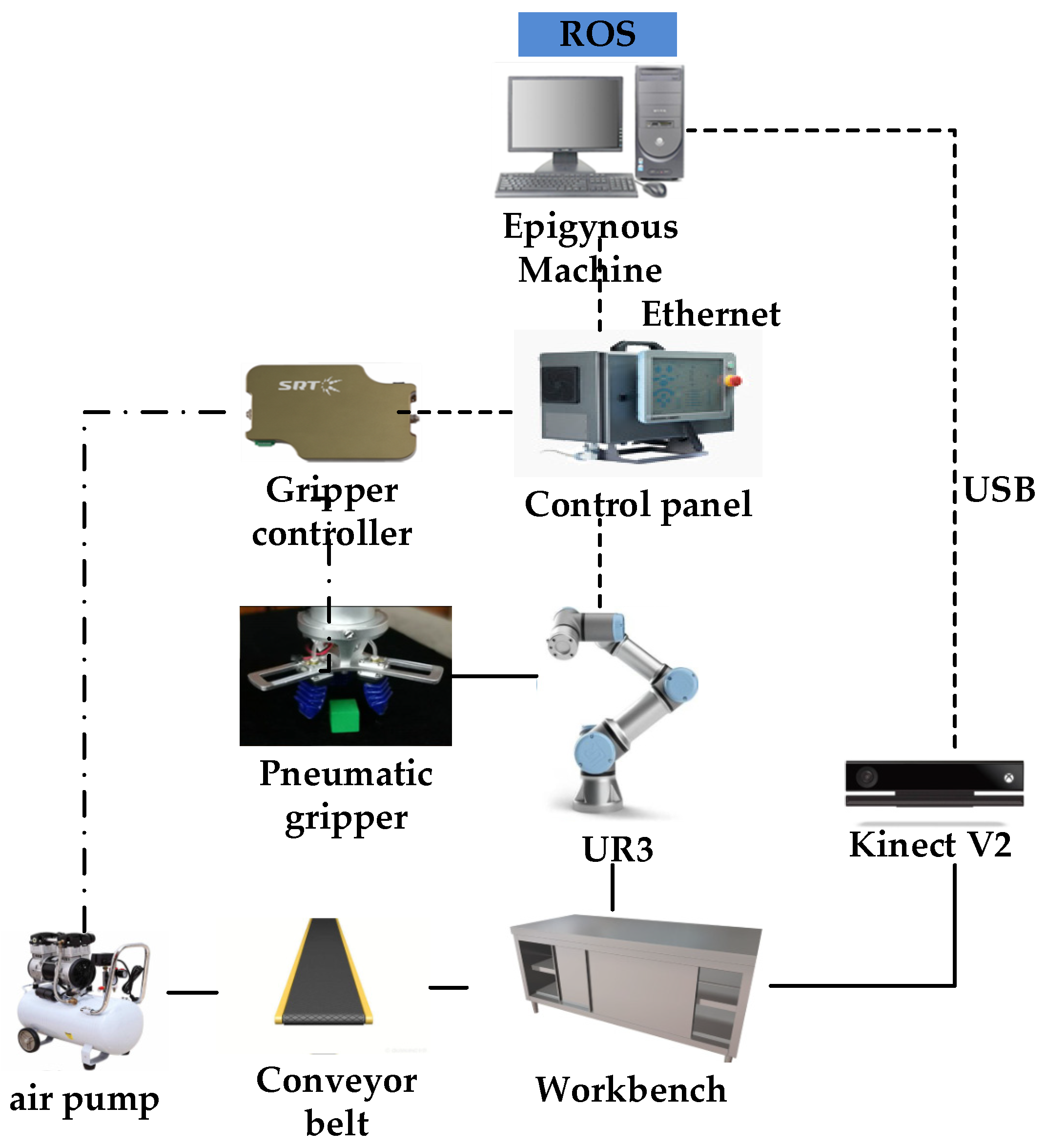
In this paper, the experimental platform is built according to the research needs. The robot’s dynamic tracking and the grasping system are shown in Figure 2. The system includes the upper computer, the UR3 robot, the control cabinet, the SRT pneumatic software gripper, the pneumatic control board, the air pump, and the Kinect2. It is composed of a camera, workbench, and conveyor belt.

The Kinect V2 depth camera collects the color image and depth image of the object. It sends the obtained image information to the upper computer. The hypogynous machine uses the Ubuntu16.04 operating system and the ROS robot system to process the image information obtained by the depth camera to provide preparation for the dynamic tracking algorithm. The upper computer combines the algorithm to send the UR3 robot controller through the TCP/IP protocol. The UR3 controller controls the robot to perform the grasping action.

4.2. Target Tracking Method Comparison Experiment

In order to compare the tracking performance of IGPF, GPF and PF, the TB-50 sequences in the OTB2015 dataset were used. These 50 video images contained 11 typical cases. They are occlusion (OCC), illumination variation (IV), low resolution (LR), motion blur (MB), fast motion (FM), out-of-view (OV), deformation (DEF), background clutter (BC), scale variation (SV), in-plane rotation (IPR) and out-of-plane rotation (OPR).

The evaluation indicators used are the distance precision (DP) and overlap success (OS) of the OTB platform. The time and space robustness of the algorithm are also key indicators. Hence, there are three different evaluation methods for DP and OS, respectively. They are one-time pass evaluation (OPE), time robustness evaluation (TRE) and space robustness evaluation (SRE). The DP refers to the difference between the center position of the target obtained by the tracking algorithm and the real position of the human mark, expressed in Euclidean distance, and its unit is a pixel. The OS is the area ratio of the intersection of the target bounding box obtained by the value tracking algorithm and the manually marked target bounding box of the data set and the area of the union set. It can be expressed by the following formula:

$$OS=\frac{\left|S_C{{\displaystyle \cap }}^{ }{S}_T\right|}{\left|S_C{{\displaystyle \cup }}^{ }{S}_T\right|}$$

(31)

Among them, CS represents the target bounding box obtained by the tracking algorithm, TS represents the true value of the manually marked target bounding box, the calculation of the intersection of the two bounding boxes, and the calculation of the union of the two bounding boxes.

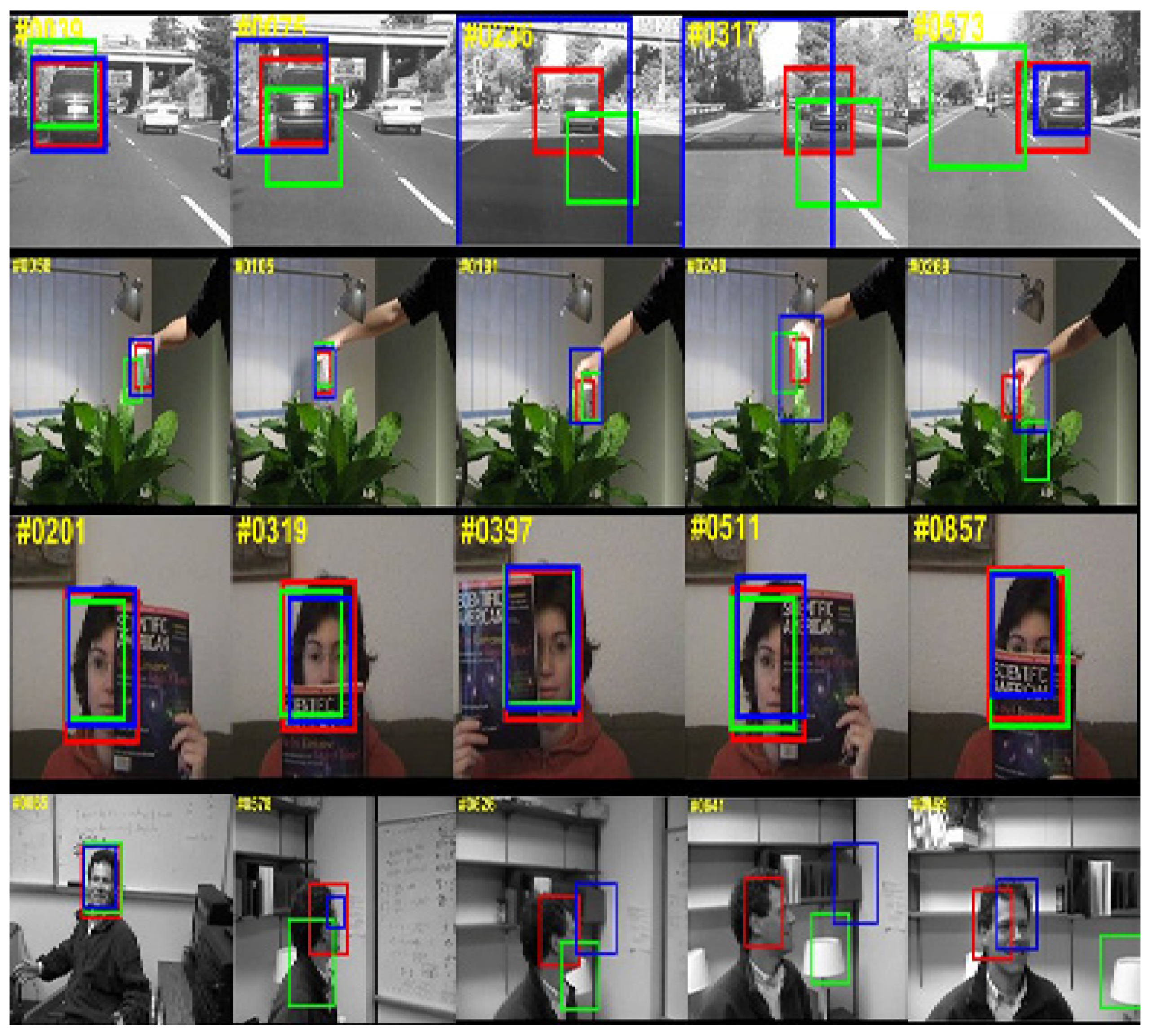
The three algorithms are compared according to the above evaluation method on the OTB2015-TB50 dataset. Screenshots of some video frames are selected to perform the comparison, as shown in Figure 3. From the figure, it can be seen that the IGPF algorithm represented by the red box has better tracking performance than GPF (blue box) and PF (green box) in grayscale and color images with occlusion and insufficient light.

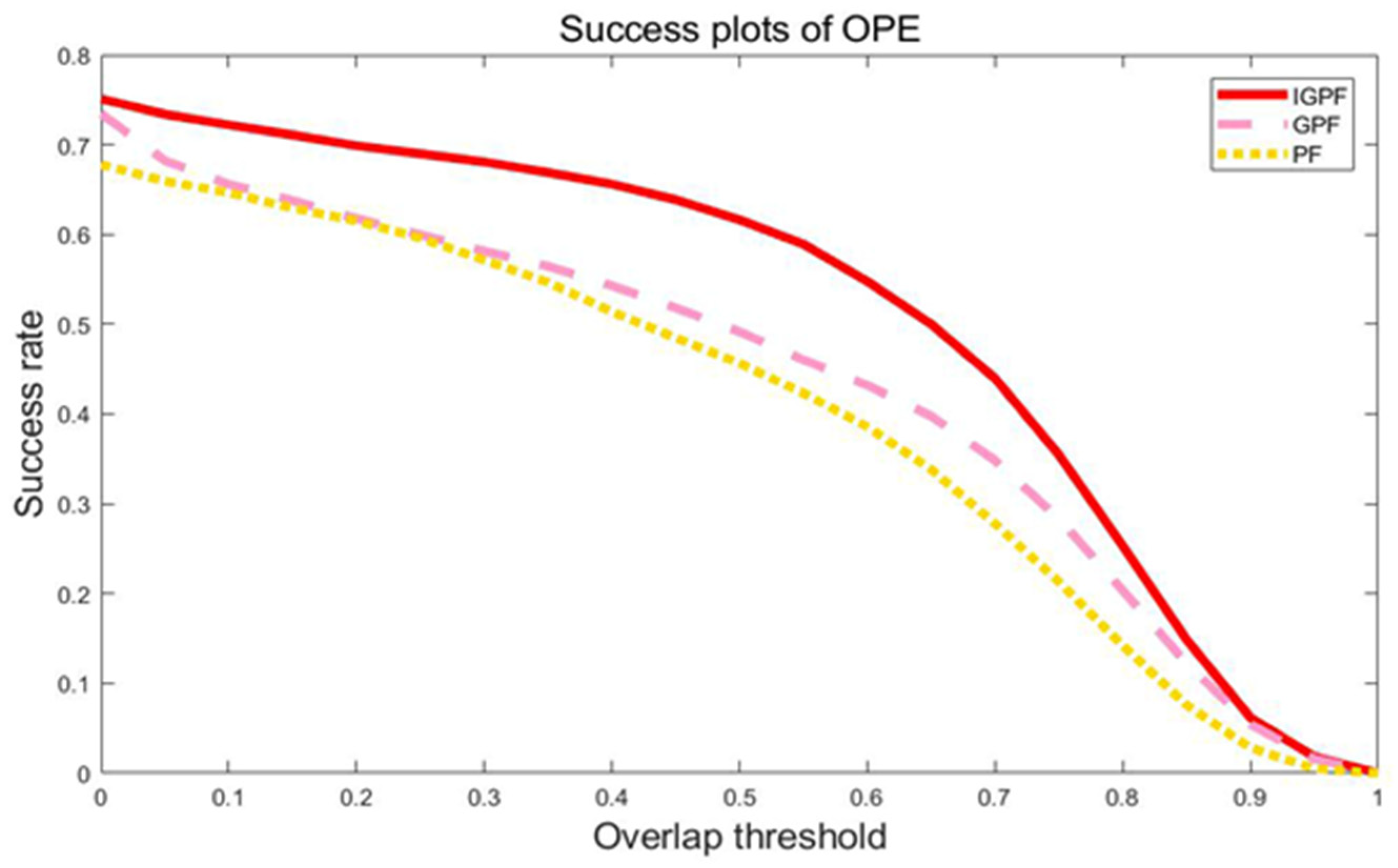
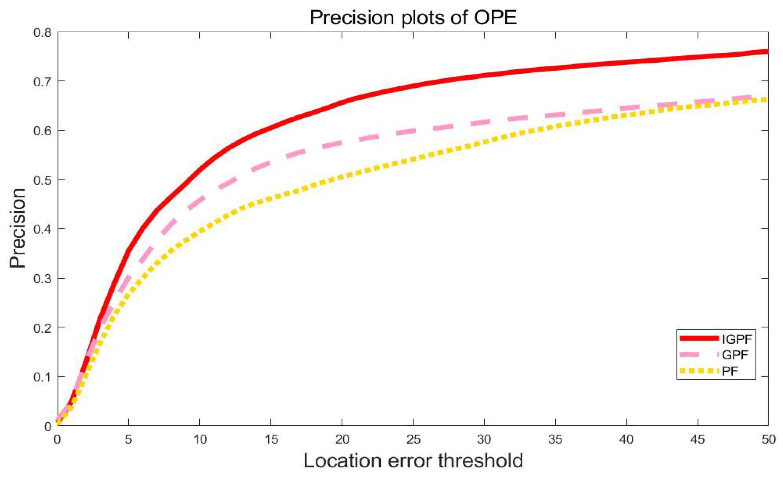
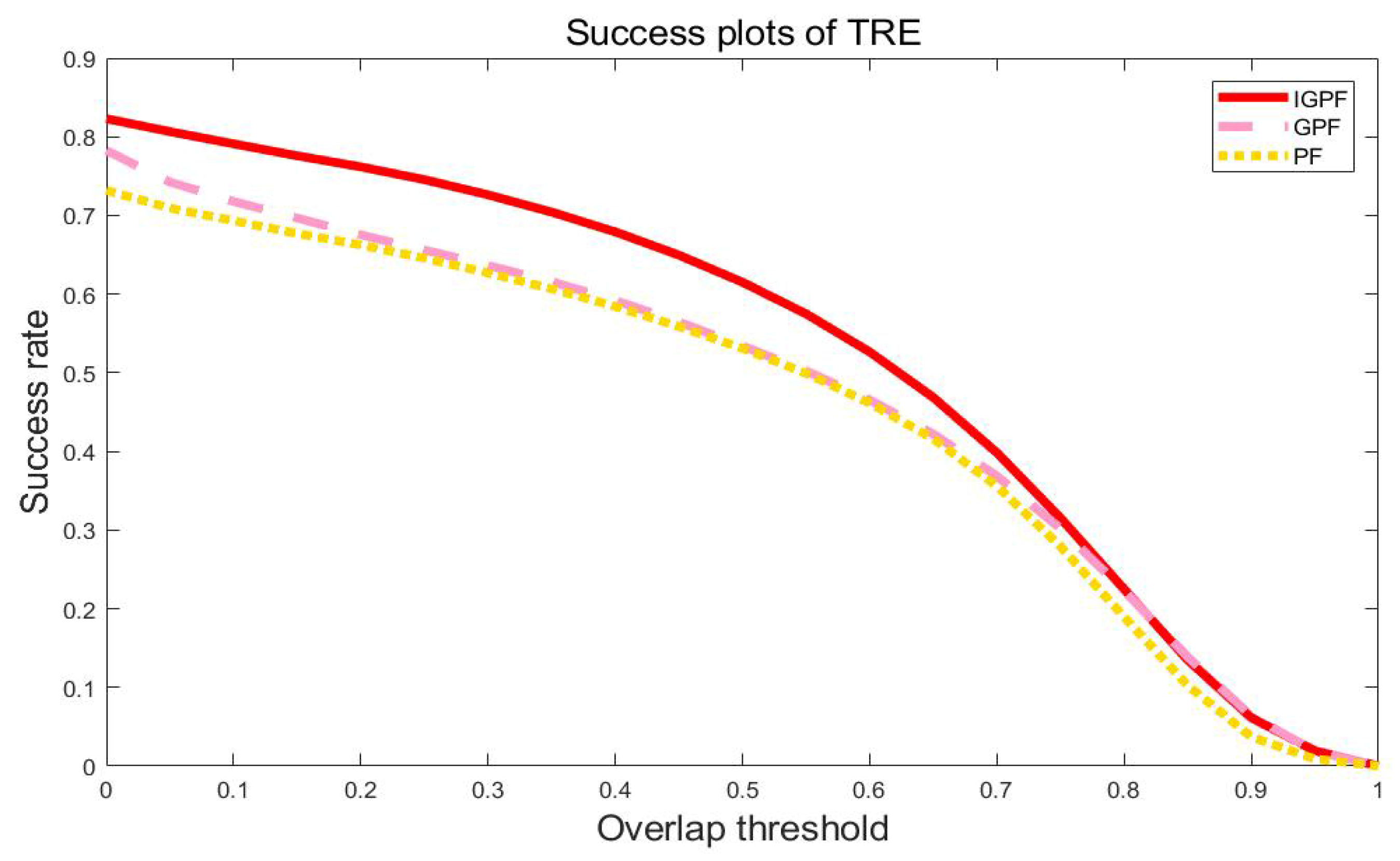
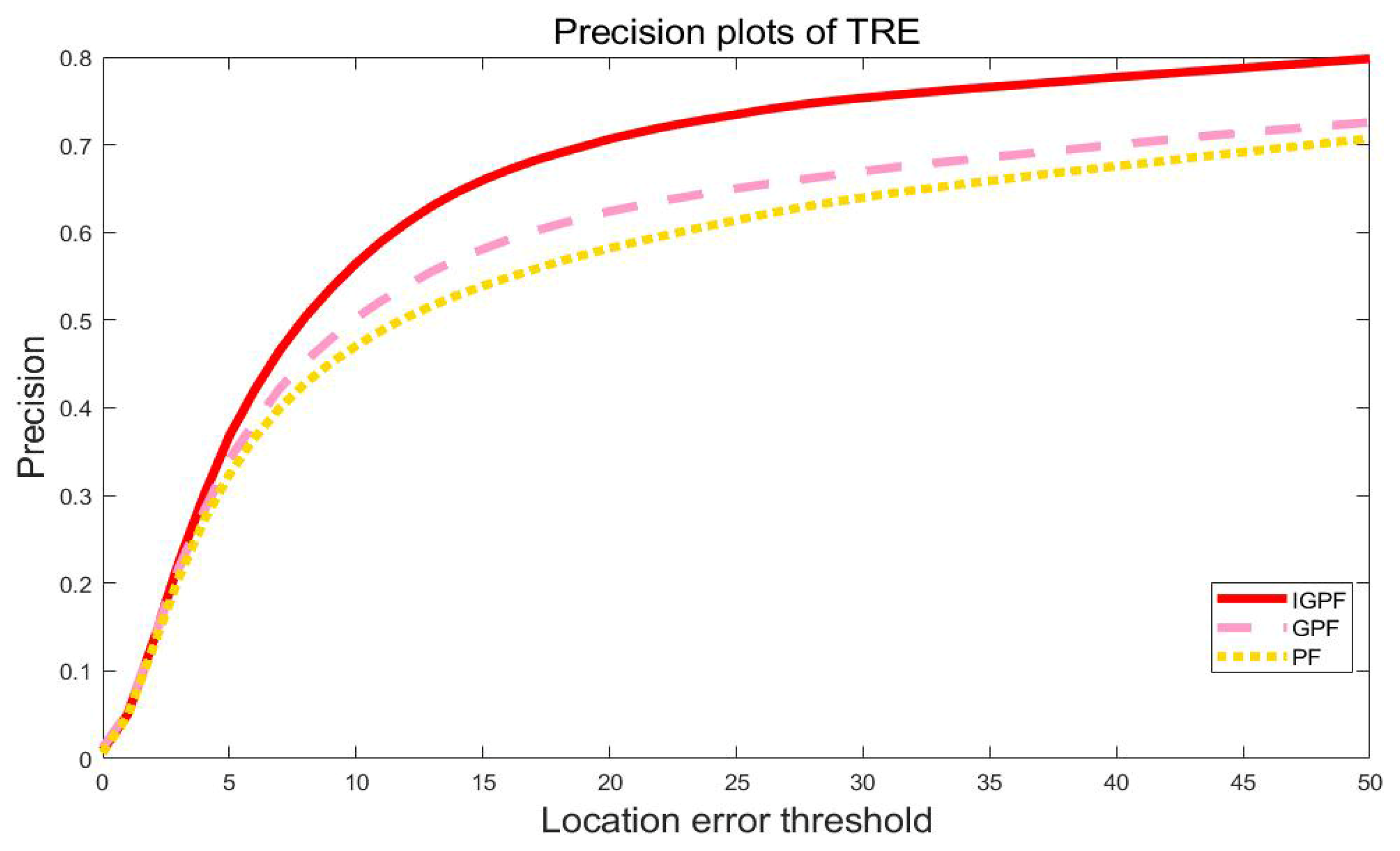
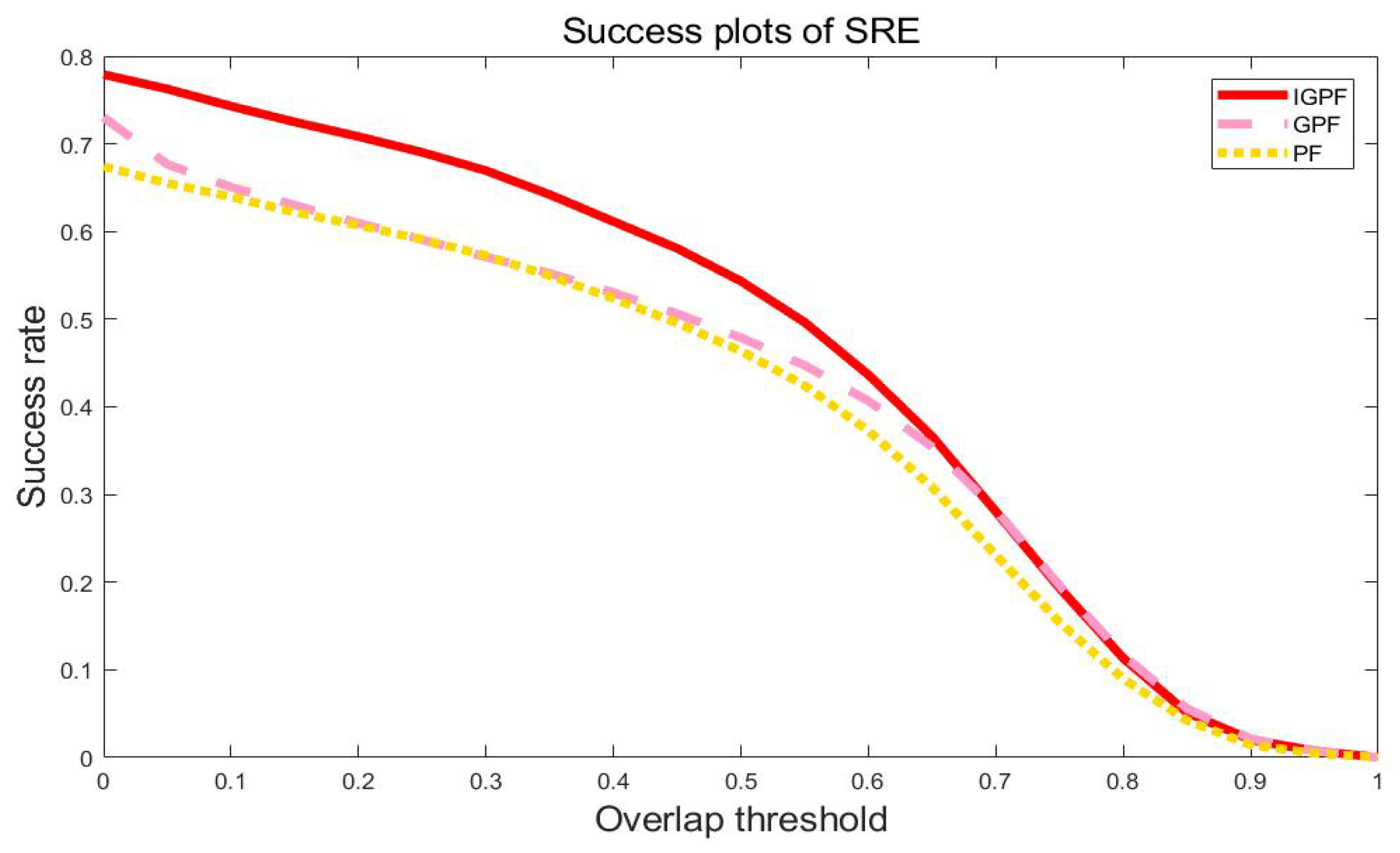
The obtained DP curve and OS curve are shown in Figure 4, Figure 5, Figure 6, Figure 7, Figure 8 and Figure 9. The improved GPF algorithm has better time robustness, space robustness and OS than the conventional PF algorithm and GPF algorithm. The OPE means that the tracking algorithm takes the first frame in the test image sequence as the initial frame and the real position of the first frame as the initial position and then tracks the subsequent images. The TRE refers to taking different frames in the image sequence as the initial frame and the real position of the frame as the initial position and then tracking the subsequent images. The TRE is usually performed 20 times. The images at different moments are initialized, and then the subsequent images are tracked. The SRE refers to taking the first frame in the test image sequence as the initial frame but changing the real position of the first frame as the initial position so that the initial position is not at the real position. Bottom, left, right, top left, top right, bottom left and bottom right are translated in eight directions. The amount of translation is 10% of the target size. In addition, it also contains four different scales of 0.8, 0.9, 1.1 and 1.2, totaling. After 12 tests, draw the center position error curve and the overlap success rate error curve.

The DP rate average and OS average of the three algorithms are calculated. The performance improvement rate of the IGPF algorithm relative to the GPF algorithm is also calculated. The results are shown in

Table 1. Initial parameter setting of algorithm.

	OPE Average	TRE Average	SRE Average
PF	0.540	0.447	0.494
GPF	0.618	0.556	0.530
IGPF	0.690	0.645	0.617
Improvement rate	11.65%	16.01%	16.42%

and

Table 2. OS comparison of the three algorithms.

	OPE Average	TRE Average	SRE Average
PF	0.561	0.501	0.565
GPF	0.664	0.613	0.638
IGPF	0.746	0.724	0.767

. It can be seen that the evaluation (OPE), robustness (TRE) and space robustness (SRE) are improved by more than 10%. Moreover, the differences between the TRE average and the OPE average of the DP and OS of the IGPF algorithm are significantly smaller. It indicates that IGPF is less affected by the start frame and initial position settings.

4.3. Robot Grasping Experiment

4.3.1. Experiments in a Normal Environment

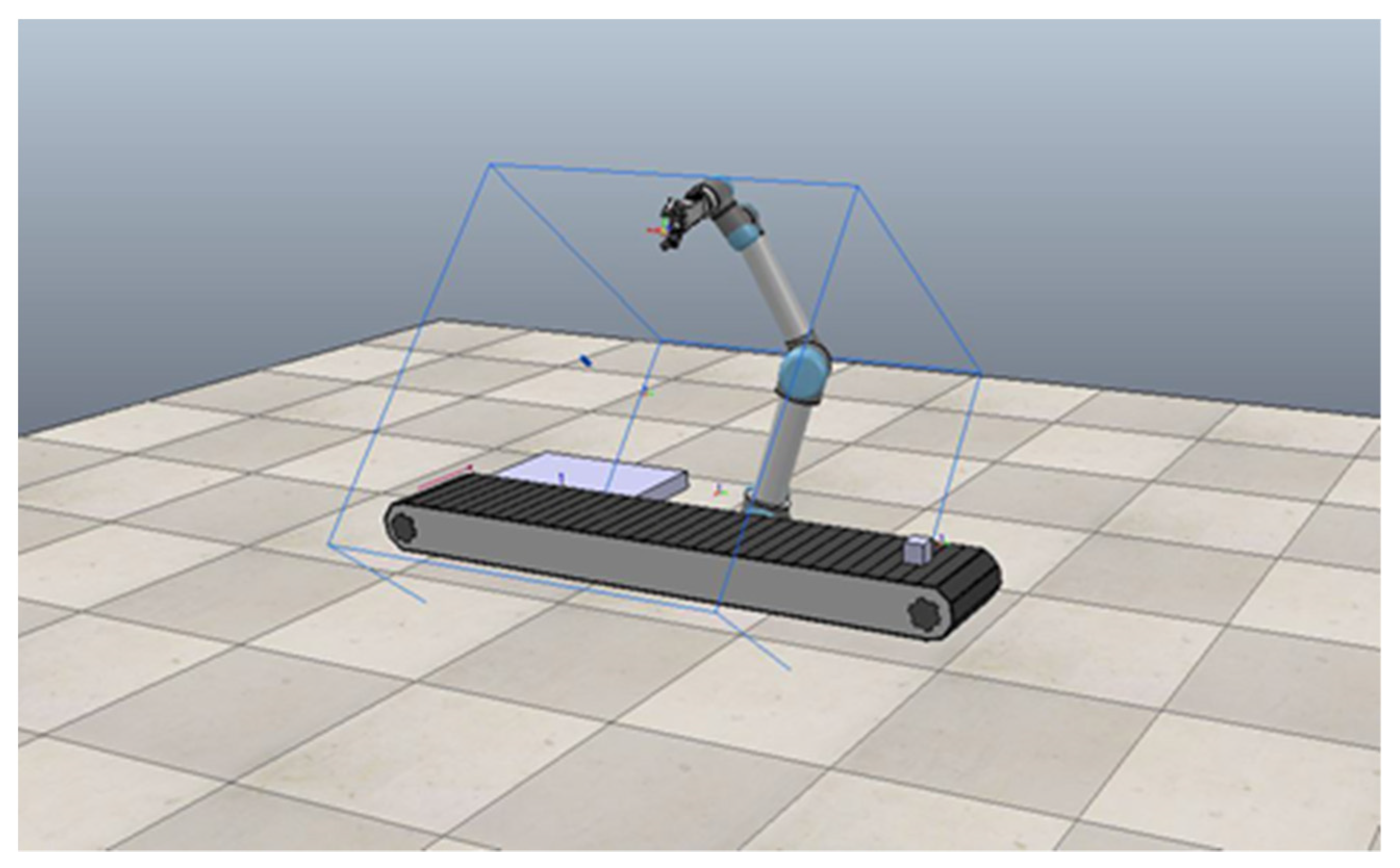
In order to verify the application feasibility of the algorithm in robot grasping, an experimental environment in CoppeliaSim is presented, as shown in Figure 10. It includes a UR5 robotic arm, RG2 gripper, conveyor belt and vision sensor. The objects used in the experiment are all the same ordinary cuboid. The cuboid is a rigid body whose size is 20 × 8 × 8 cm. The manipulator can track until the grabbed object leaves the conveyor belt and it is deemed successful.

Firstly, the conveyor belt is in a state of uniform linear motion. The target starts to move from the starting point of the conveyor belt. The repeated experiments are carried out at different speeds of the conveyor belt. The initial state of each experiment is the same. The continuous tracking image in the experiment is shown in Figure 11. The crawling success rate and average tracking time at different speeds are shown in

Table 3. Tracking and Grasping results of uniform linear moving target.

Velocity (m/s)	Number of Experiments	Success Rate (%)	Average Tracking Time (s)
0.1	50	88	1.2
0.15	50	82	2.5
0.25	50	76	3.0

.

According to Table 3, the algorithm has a higher success rate at 0.1 m/s, and after exceeding 0.15 m/s, the success rate drops more. As the speed increases, the tracking distance of the robotic arm increases.

The experimental platform in the real environment is similar to the simulation environment. It consists of UR3 robots, conveyor belts and cameras. Figure 12 shows the images continuously captured by the camera in the mobile production line tracking and grabbing experiment. The camera detects the target and the end pose of the robot starts to move. The pose of the target approaches, and the robotic arm tracks the target for synchronous follow-up until it meets the grasping conditions to achieve grasping.

Similar to the simulation experiment, the real environment experiment also sets different conveyor speeds to repeat the experiment. Each experiment ensures that the initial pose of the robotic arm is the same. The initial pose of the target is the same. The conveyor speed is set to 0.1 m/s, 0.15 m/s and 0.25 m/s, respectively. The 50 grasping experiments are carried out, respectively. The statistical experiment grasping success rate and average tracking time is proposed. The experimental results are shown in

Table 4. Real environment tracking and grasping results.

Velocity (m/s)	Number of Experiments	Success Rate (%)	Average Tracking Time (s)
0.1	50	84	2.4
0.15	50	78	3.7
0.25	50	74	4.4

.

Then, the experimental data were further analyzed. The Euclidean distance between the target and the robot at the same time is calculated in the base coordinate system as the error, which is the ordinate of the curve. The horizontal axis represents the experimental time for the error to converge below the threshold. The error curve at different speeds is proposed. In the experiment, the minimum velocity of 0.1 m/s and the maximum velocity of 0.25 m/s draw error curves, respectively, as shown in Figure 13. Both thresholds are 0.1.

As shown in the figures, the rate of change of the two-speed error curves shows a trend from large to small to large. It corresponds to the change from the acceleration of the robot’s motion to the final stable tracking during the robot tracking process. Finally, the error has converged to below the set threshold. It proves the effectiveness of the robot dynamic target capture algorithm based on affine group improved Gaussian resampling particle filter proposed in this paper.

Since we used the average error of 50 repeated experiments in Figure 13, the grasping error during the 50 experiments fluctuates. The error bars are shown in Figure 14. The left side is 0.1 m/s and the right side is 0.25 m/s. The position where the error fluctuates sharply is also the position where the error bar is large, basically at the stage where the reverse osmosis arm quickly approaches the target from the distal end. During this period, the error appears to fluctuate greatly due to the inverse kinematics solution and tracking algorithm. In the initial stage and the final crawling stage, the error bar is very small, which meets the experimental requirements.

4.3.2. Experiments in Extreme Environments

As the typical situation mentioned in Section 4.2, we selected two situations of low resolution (LR) and illumination variation (IV) to carry out tracking and grasping experiments. We completed the tracking and grabbing experiments at low resolution, as shown in Figure 15. Only part of the natural light was retained. The entire experiment was carried out in a low-light environment. In addition, we conducted an experiment on the resolution change of the indoor environment from good to dark during the tracking and capturing process, as shown in Figure 16.

The experiment settings were consistent with the previous experiments. The 50 crawling experiments were still carried out at different speeds. The crawling success rate and average tracking time in the two cases were counted. The experimental results are shown in

Table 5. Low resolution tracking and grasping results.

Velocity (m/s)	Number of Experiments	Success Rate (%)	Average Tracking Time (s)
0.1	50	80	3.4
0.15	50	76	4.5
0.25	50	70	5.2

and

Table 6. Illumination variation tracking and grasping results.

Velocity (m/s)	Number of Experiments	Success Rate (%)	Average Tracking Time (s)
0.1	50	82	3.0
0.15	50	78	4.2
0.25	50	74	4.8

.

From the Tables, it can be seen that both low resolution and illumination variation have an impact on the experimental result. It can be seen that the tracking algorithm based on the image input of the optical device is more sensitive to light. The success rate of illumination variation is slightly higher than that of low resolution. It indicates that the accuracy rate in the tracking process has a positive effect on the final capture success rate. Experimental results in both cases show the effectiveness of the proposed algorithm.

5. Conclusions and Discussion

This paper is oriented to robot tracking and grabbing of dynamic targets based on previous work and the GPF framework. The affine groups are proposed as particles. In response to the problem of insufficient particle diversity, the Gaussian resampling is fused in the resampling and improved. The low-weight particles and preliminary resampled particles are combined to reduce the difference in the particle probability distribution before and after resampling to improve particle diversity. It improves the tracking performance. The difference between the 3D pose of the dynamic target and the end 3D pose is calculated. The end of the robot is adjusted in real time to approach the dynamic target. A robot dynamic target tracking and grasping method are proposed based on the affine group and improved Gaussian resampling particle filter. Finally, the particle filter algorithm, geometric particle filter algorithm and the improved geometric particle filter algorithm are used to select suitable videos for experimental verification in an environment where a variety of robots are more closely grasped. The robot is used in the simulation environment and the actual environment to perform the robot against the dynamic target. A grabbing simulation and experiment were conducted to realize the robot’s prediction and grasping of dynamic targets. The simulation in the simulation environment proves that the algorithm spends less time on tracking and has high efficiency, and the experimental results prove the effectiveness of the proposed method.

The currently defined grasping posture is perpendicular to the target surface and for simple objects with regular shapes. There is no in-depth consideration of the posture planning of complex-shaped objects. The tracking algorithm is to track the two-dimensional plane of the target. The occurrence of occlusion will still affect the tracking effect, although the algorithm has actually improved the occlusion tracking. In the future, the existing limitations will be studied and improved.

The experiment did not observe the tracking of objects in three-dimensional space. The tracking algorithm only verified the simple movement of the two-dimensional plane in the real environment. When considering the three-dimensional pose of the object in a real-time state, the real-time performance of the algorithm and the solution of the hardware platform’s mathematical ability is a challenge. The future work will focus on three-dimensional object tracking and verify the generalization and effectiveness of the algorithm in extreme cases such as parabolic real-time tracking and occlusion in unstructured environments.