Fractional-Order PII^1/2DD^1/2 Control: Theoretical Aspects and Application to a Mechatronic Axis

Featured Application

PII^1/2DD^1/2 control can replace PID control in any application, enhancing its performance. In the present paper, the investigation is focused on the control of mechatronic systems, in particular actuated rotational joints, but the findings can be easily extended to actuated translational joints.

Abstract

Fractional Calculus is usually applied to control systems by means of the well-known PI^λD^μ scheme, which adopts integral and derivative components of non-integer orders λ and µ. An alternative approach is to add equally distributed fractional-order terms to the PID scheme instead of replacing the integer-order terms (Distributed Order PID, DOPID). This work analyzes the properties of the DOPID scheme with five terms, that is the PII^1/2DD^1/2 (the half-integral and the half-derivative components are added to the classical PID). The frequency domain responses of the PID, PI^λD^μ and PII^1/2DD^1/2 controllers are compared, then stability features of the PII^1/2DD^1/2 controller are discussed. A Bode plot-based tuning method for the PII^1/2DD^1/2 controller is proposed and then applied to the position control of a mechatronic axis. The closed-loop behaviours of PID and PII^1/2DD^1/2 are compared by simulation and by experimental tests. The results show that the PII^1/2DD^1/2 scheme with the proposed tuning criterium allows remarkable reduction in the position error with respect to the PID, with a similar control effort and maximum torque. For the considered mechatronic axis and trapezoidal speed law, the reduction in maximum tracking error is −71% and the reduction in mean tracking error is −77%, in correspondence to a limited increase in maximum torque (+5%) and in control effort (+4%).

1. Introduction

Fractional Calculus (FC) is the generalization of the concepts of derivative and integral from integer to non-integer order [1]. The origin of FC dates back even to the seventeenth century: as a matter of fact, it was discussed by De L′Hopital, Leibniz, Euler, Fourier, Liouville and Riemann. The birth and the historical development of FC are outlined in [2]. After a long period of being forgotten, in the last few decades there has been a renewed research interest in FC, also due to the discovered relationship with the chaos theory. Some real systems can be better modelled by Fractional Order (FO) equations than by Integer Order (IO) ones, in particular in the case of multi-scale problems, with wide dimensional or time scales, as found, for example, in viscoelasticity problems [3,4]. FC is used to provide more accurate models in mechanics [5], physics [6] and biology [7]. Recently, FC has been used to model the evolution of the COVID-19 pandemic [8,9].

Nowadays FC is not only used as modelling tool, but also in engineering applications, and in particular in the field of control system design. Most control algorithms are based on IO derivatives and integrals of the error; the extension to FO derivatives and integrals introduces additional parameters which can be tuned to improve the closed-loop system performance.

The most widespread approach to apply FC to control system design is the well-known PI^λD^μ scheme, which adopts integral and derivative terms of non-integer orders λ and µ [10]. Design techniques, optimization tools and practical applications of PI^λD^μ controllers are widely discussed in the scientific literature. Some approaches are derived from classical tuning criteria: in [11] tuning is obtained by modified Ziegler–Nichols and Astrom–Hagglund methods, while in [12] the classical isodamping condition is generalized for the PI^λD^μ controller. Other approaches are based on numerical optimization techniques, for example Artificial Bee Colony algorithms [13], Particle Swarm Optimization [14] or optimal shaping of the Bode plot to achieve robustness [15]. In [16] a population-based optimization approach named the Sine–Cosine Algorithm is applied to PI^λD^μ generation control in wind farms. In [17] an optimized PI^λD^μ controller is compared to the Linear Quadratic Gaussian and H∞ controllers. The robustness to parametric uncertainties and the rejection of external disturbances is considered in [18,19].

The application of PI^λD^μ can greatly improve the performance in the transient behavior for motion control applications, for example in case of mechatronic devices actuated by DC motors. In [20] PI^λD^μ is used for speed control of a buck converter-fed DC motor. In [21] an analog implementation exploiting the Operational Transconductance Amplifier is used for controlling a DC motor. In [22] PI^λD^μ is applied to speed control of a chopper-fed DC motor drive. Chaotic Atom Search Optimization [23] and Flower Pollination Algorithms [24] are proposed to tune the PI^λD^μ parameters for DC motor speed control. In [25] a methodology for the quantitative robustness evaluation of PI^λD^μ controllers employed in DC motors is proposed. In [26] an inertial load elastically connected to a DC motor is studied, comparing IO and FO controllers. Other works are related to the application of PI^λD^μ to different actuators, for example synchronous motors [27], linear motors [28,29], linear positioning systems [30].

Besides the PI^λD^μ scheme, FC can be profitably applied to control system design in different ways, for example for enhancing the performance of sliding mode control by applying a FO disturbance observer [31]. In [32], a sliding mode backstepping control method is proposed, which involves the use of a fractional-order command filter, a fuzzy logic system approximator, and a grey wolf and weighted whale optimization algorithm for multi-input multi-output nonlinear dynamic systems.

Instead of replacing the IO terms as in the PI^λD^μ scheme, an alternative way to apply FC to control systems is to add FO terms to the PID scheme. This approach was introduced in 2009 by Bruzzone et al. [33] with the PDD^1/2 scheme, in which a half-derivative term is added to the classical PD controller. In [34] the dynamic behavior of the PDD^1/2 control in combination with a purely inertial system is discussed, adopting a nondimensional approach. In [35] the PDD^1/2 scheme is applied in simulation to position control of a non-linear multi-input multi-output plant (a Parallel Kinematics Machine). The effectiveness of the PDD^1/2 scheme has been experimentally validated in the position control of a micrometric linear axis [36] and of a rotor [37]. In [38] the PD, PD^μ and PDD^1/2 controls of a purely inertial system are compared by simulation, and the results indicate that the two FO schemes have similar performance, but the PDD^1/2 is characterized by a slightly better readiness and a slightly higher overshoot. In [39] the comparison among PD, PD^μ and PDD^1/2 is validated by experimental tests, highlighting the benefits of the proposed control approach in real working conditions, not limited to the classical step response.

The proposed PDD^1/2 scheme did not include an integral action, as the focus of the research was the optimization of the transient behavior of the system. Compared to the PD performances, with the same control effort, the introduction of the half-derivative term reduces the transient tracking error, also in case of complex MIMO nonlinear mechanical systems, with possible applications in position, force or impedance control [40] of serial and parallel robots.

In 2017, a similar approach has been proposed by Jakovljevic et al. and named Distributed Order PID (DOPID) [41], and then applied to the control of permanent magnet synchronous motor drives [42,43]. In the DOPID_N, the control action is given by the linear combination of an odd number n (with n ≥ 3) of differintegrators of equally spaced orders ranging from −1 to +1. Accordingly, for n = 3, the DOPID₃ corresponds to the classical PID, since the three differintegration orders are −1, 0, +1. For n = 5, the DOPID₅ orders are −1, −1/2, 0, +1/2, +1, etc. The PDD^1/2 scheme is a subcase of DOPID₅ with null integral gains.

In the present paper the integral terms are added to the PDD^1/2 controller, to obtain a more general control scheme, capable of providing the required accuracy also in a steady state. Therefore, three control schemes are compared: the classical integer-order PID, the fractional-order PI^λD^μ and the PII^1/2DD^1/2, which corresponds to DOPID₅, while in [41,42,43] the DOPID₇ is mainly considered.

In the following of the paper:

-

the integro-differential operator and its discrete-time approximation are recalled in Section 2;

-

the formulation of the PII^1/2DD^1/2 control scheme is outlined and its transfer function is compared to the ones of PID and PI^λD^μ in Section 3;

-

the frequency domain response of the three controllers is discussed in Section 4;

-

Section 5 debates the stability properties of closed-loop systems with IO plant and PII^1/2DD^1/2 control;

-

a Bode plot-based tuning method for the PII^1/2DD^1/2 control is proposed (Section 6) and then applied to position control of a rotor, comparing the performances of PID and PII^1/2DD^1/2 by continuous-time simulation (Section 7);

-

for the same case study, the performances of the controllers are then compared considering a real implementation with finite sampling time and finite memory length of the digital filters; this analysis is carried out both by discrete-time simulation and by experimental tests (Section 8);

-

Section 9 and Section 10 outline conclusions, related work, and future developments.

2. The Integro-Differential Operator

In FC the same continuous integro-differential operator ${}_{a}D_t^{\alpha }$ represents both integration and differentiation to a non-integer order:

$${}_{a}D_t^{\alpha }=\{\begin{array}{cc}{d}^{\alpha }/d{t}^{\alpha }\hfill & \mathrm{Re}\left(\alpha \right)>0\hfill \\ 1\hfill & \mathrm{Re}\left(\alpha \right)=0\hfill \\ {\displaystyle \underset{a}{\overset{t}{\int }}{\left(d\tau \right)}^{-\alpha }}\hfill & \mathrm{Re}\left(\alpha \right)<0\hfill \end{array}$$

(1)

In Equation (1) a and t are the limits of the operation and α is the order, which can be real or complex; in the following, α ∈ R. In the scientific literature several definitions of the integro-differential operator have been proposed (Grünwald–Letnikov, Riemann–Liouville, Tustin, Simpson, Caputo, among the others) [2], but all of these are proved to be equivalent [44]. In the following the Grünwald–Letnikov definition is adopted, since it leads to a robust discrete-time implementation [45].

According to the Grünwald–Letnikov definition, the differentiation of fractional order α (if α > 0) or the integration of fractional order −α (if α < 0) of a function of time x(t) is defined as:

$${}_{a}D_t^{\alpha }x\left(t\right)=\underset{h\to 0}{\lim }[\frac{1}{h^{\alpha }}{\displaystyle \sum _{k=0}^{\left[\frac{t-a}{h}\right]}{\left(-1\right)}^k}\frac{\Gamma \left(\alpha +1\right)}{\Gamma \left(k+1\right)\Gamma \left(\alpha -k+1\right)}x\left(t-kh\right)]$$

(2)

where h is the time increment and Γ is the Gamma function, which extends the factorial function to real and complex numbers and is defined by the following equation:

$$\Gamma \left(z\right)={\displaystyle \underset{0}{\overset{\infty }{\int }}{t}^{z-1}{e}^{-t}dt}$$

(3)

In order to understand intuitively the meaning of FO derivatives and integrals, independently of their mathematical definition, we can consider the following properties:

-

similarly to IO derivatives and integrals, if an FO derivative/integral of order α is applied twice to a function of time, the resulting function is the derivative of order 2α; for example, the derivative of order 1/2 of the derivative of order 1/2 is the first-order derivative, and the integral of order 1/2 of the integral of order 1/2 is the first-order integral;

-

for sinusoidal functions, similarly to IO derivatives/integrals, FO derivatives/integrals of order α produce a phase shift of απ/2: for example, the first-order derivative causes a positive phase shift of π/2, while the derivative of order 1/2 causes a positive phase shift of π/4; the first-order integral causes a negative phase shift of π/2, while the integral of order 1/2 causes a negative phase shift of π/4.

In Equation (2) the number of terms of the sum tends towards infinity, since h tends towards zero; for a discrete-time numerical computation, Equation (2) can be rewritten adopting a small but finite sampling time T_s, in order to obtain the following discrete-time approximation [46]:

$$D_t^{\alpha }x\left(t\right)\cong D^{\alpha }{x}_k=\left[\frac{1}{T_s^{\alpha }}{\displaystyle \sum _{j=0}^k{w}_j^{\alpha }}x\left(t-j{T}_s\right)\right]$$

(4)

where k = (t − a)/T_s is the current step and:

$$\begin{array}{l}{w}_0^{\alpha }=1\\ w_j^{\alpha }=\left(1-\frac{\alpha +1}{j}\right)w_{j-1}^{\alpha } , j=1, 2, \dots \end{array}$$

(5)

For real-time implementation on a digital controller, for t >> a the number of addends becomes too large; therefore, it is necessary to limit the number of considered steps, in order to have a computational burden compatible with the controller CPU. Therefore, at each time step a fixed number n of previous steps is considered in (4), with n < k; this corresponds to the application of a nth order digital filter, which can be rewritten in terms of z-transfer notation:

$$D^{\alpha }\left(z\right)=\left[\frac{1}{T_s^{\alpha }}{\displaystyle \sum _{j=0}^n{w}_j^{\alpha }}{z}^{-j}\right]$$

(6)

The memory length of this filter, L = nT_s, is fixed; fortunately, as time advances, the oldest part of the history of the function x(t) becomes negligible for the short-memory principle [2], therefore taking into account only the recent past of the function, in the interval [t − L, t], which does not introduce relevant approximations in the evaluation of the FO derivatives and integrals.

3. The PII^1/2DD^1/2 Control Scheme

To introduce the proposed PII^1/2DD^1/2 control, let us consider a second-order plant (Figure 1). Many mechatronic systems in which friction can be considered viscous can be suitably modelled by a second-order linear system. In the following a rotor with inertia J and viscous coefficient B driven by a torque M commanded by the controller will be considered.

The open-loop plant dynamics is expressed by the following differential equation:

$$J\frac{d^2}{d{t}^2}\theta +B\frac{d}{dt}\theta =M\left(e_{\theta }\right)$$

(7)

where M is the controller output, calculated as a function of the error e_θ, difference between the set-point angle θ_r and the current angle θ.

In the following, for the closed-loop control scheme of Figure 1, three control laws will be considered: the integer-order PID, the fractional-order PI^λD^μ and the proposed PII^1/2DD^1/2.

The classical PID control law is based on the well-known proportional, integral and derivative gains K_p, K_i, K_d:

$$M\left(e_{\theta }\right)=(K_p+K_i{D}^{-1}+K_d{D}^1)e_{\theta }$$

(8)

In case of PI^λD^μ, the control law is given by:

$$M\left(e_{\theta }\right)=\left(K_p+K_{fi}{D}^{-\lambda }+K_{fd}{D}^{\mu }\right)e_{\theta }$$

(9)

where K_p, K_fi and K_fd are the proportional, fractional-order integral and fractional-order derivative gains, λ is the fractional integral order and µ is the fractional derivative order [10].

Similarly to the PDD^1/2 concept, in which the half-derivative term is added to the derivative one instead of replacing it with an FO derivative term, in the proposed PII^1/2DD^1/2 control the half-derivative and the half-integral terms are added to the PID; therefore, the PII^1/2DD^1/2 control law is:

$$M\left(e_{\theta }\right)=\left(K_p+K_i{D}^{-1}+K_{hi}{D}^{-1/2}+K_d{D}^1+K_{hd}{D}^{1/2}\right)e_{\theta }$$

(10)

where K_hd is the half-derivative gain and K_hi is the half-integral gain.

Applying a Laplace transform to Equations (8) to (10) with null initial condition, the transfer functions of the three controllers can be expressed by:

$$G_{c,PID}(s)=K_p+\frac{K_i}{s}+K_{d}s=K_i\frac{\left(1+\left(K_p/K_i\right)s+\left(K_d/K_i\right)s^2\right)}{s}$$

(11)

$$G_{c,P{I}^{\lambda }{D}^{\mu }}(s)=K_p+\frac{K_{fi}}{s^{\lambda }}+K_{fd}{s}^{\mu }=K_{fi}\frac{\left(1+\left(K_p/K_{fi}\right)s^{\lambda }+\left(K_{fd}/K_{fi}\right)s^{\lambda +\mu }\right)}{s^{\lambda }}$$

(12)

$$\begin{array}{l}{G}_{c,PI{I}^{1/2}D{D}^{1/2}}(s)=K_p+\frac{K_i}{s}+\frac{K_{hi}}{s^{1/2}}+K_{d}s+K_{hd}{s}^{1/2}=\\ =K_i\frac{1+\left(K_{hi}/K_i\right)s^{1/2}+\left(K_p/K_i\right)s+\left(K_{hd}/K_i\right)s^{3/2}+\left(K_d/K_i\right)s^2}{s}\end{array}$$

(13)

Let us note that while the PID has three degrees of freedom for tuning (the three gains), both the FO controls have five degrees of freedom for tuning: three gains and two orders for PI^λD^μ, five gains for PII^1/2DD^1/2.

4. Frequency Domain Response of PID, PI^λD^μ and PII^1/2DD^1/2 Controllers

4.1. Factorization of Commensurate-Order Fractional-Order System

If all the orders of differintegration of an FO system are integer multiples of a base order q, with q ∈ R⁺; the system is of commensurate-order q [47]. As for IO controllers, the frequency response of FO controllers can be obtained by evaluating the transfer function for s = jω, with ω ∈ (0, ∞). In particular, for systems with commensurate-order q it is possible to obtain Bode plots by addition of individual contributions of terms of order q resulting from the following factorization [47]:

$$G_c(s)=k\frac{{\displaystyle \prod _{i=0}^m\left(s^q-z_i\right)}}{{\displaystyle \prod _{j=0}^n\left(s^q-p_j\right)}}, z_i\ne p_i$$

(14)

For each term (s^q − r)^±1 with r ≠ 0, the magnitude plot has a slope which starts at zero and tends towards ±q20 dB/dec for frequencies higher than the corner frequency |r|^1/q, while the phase plot starts at 0 and tends towards ±qπ/2 for frequencies higher than |r|^1/q; there is resonance for q > 1.

Given these premises, let us compare the frequency response of PID, PI^λD^μ and PII^1/2DD^1/2.

4.2. PID Frequency Response

The integer-order PID controller can be considered a system with commensurate order q = 1. Usually, the three gains are selected in order to produce two real zeros; in this case, its transfer function (11) can be rewritten as follows:

$$G_{c,PID}(s)=k\frac{\left(s-z_1\right)\left(s-z_2\right)}{s}$$

(15)

Tuning the thee gains K_p, K_i and K_d, it is possible to modify the placement of the low frequency asymptotical slope and the two corner frequencies −z₁ and −z₂ of the magnitude plot, and consequently the phase plot. Figure 2 shows in blue the PID controller frequency response for k = 10⁻³, z₁ = −10 rad/s, z₂ = −1000 rad/s, as an example. In the range between the two corner frequencies (10 ÷ 1000 rad/s) the asymptotic magnitude plot is constant.

4.3. PI^λD^μ Frequency Response

In general, the PI^λD^μ controller is not a commensurate-order system, especially if λ and µ are obtained by optimization. However, even if the factorization (14) cannot be applied, for low frequencies the magnitude slope tends towards −λ20 dB/dec and the phase to −λπ/2 rad, while for high frequencies the magnitude slope tends towards +µ20 dB/dec and the phase towards +µπ/2 rad [47].

Tuning the three gains K_p, K_fi and K_fd and the two orders λ and µ it is possible to modify the magnitude plot, with independent slopes at low and high frequencies, and consequently the phase plot, with independent asymptotic values at low and high frequencies. Figure 2 shows in yellow the PI^λD^µ controller frequency response for K_p = 1, K_fi = 4, K_fd = 0.015, λ = 0.8 and µ = 0.6. These example parameters provide a frequency response which is comparable to the one of the PID of Section 4.2 (blue) in the range 10 ÷ 1000 rad/s, but with different magnitude slopes and asymptotic phase values outside this range.

4.4. PII^1/2DD^1/2 Frequency Response

The PII^1/2DD^1/2 controller is a commensurate-order system, with order q = 1/2, and this represents an advantage with respect to the PI^λD^μ. First of all, if this controller is used in combination with an IO plant, the closed-loop transfer function has also commensurate order q = 1/2; therefore, the Matignon′s stability theorem [48] can be applied and the roots location in the complex plane gives relevant information about the system behaviour, as it will be discussed in Section 5.

The transfer function (13), applying the factorization (14), can be rewritten as follows:

$$G_{c,PI{I}^{1/2}D{D}^{1/2}}(s)=k\frac{{\displaystyle \prod _{i=1}^4\left(s^{1/2}-z_i\right)}}{s}=\frac{K_i}{s}{\displaystyle \prod _{i=1}^4\left(1-\frac{s^{1/2}}{z_i}\right)}$$

(16)

The asymptotic Bode plot is characterized by an initial magnitude slope of −20 dB/dec and an initial phase of −π/2 rad at low frequencies; after each corner frequency ω_c,i = |z_i|² the magnitude slope increases by 10 dB/dec, therefore at frequencies over the highest corner frequency the magnitude slope tends towards +20 dB/dec; the phase increases by π/4 rad after each corner frequency, and tends towards π/2 at frequencies over the highest corner frequency.

Expanding the product of Equation (16), it is possible to find a relation between the half-zeros z_i and the controller gains:

$$K_{hi}=K_i\left(-\frac{1}{z_1}-\frac{1}{z_2}-\frac{1}{z_3}-\frac{1}{z_4}\right)$$

(17)

$$K_p=K_i\left(\frac{1}{z_1{z}_2}+\frac{1}{z_1{z}_3}+\frac{1}{z_1{z}_4}+\frac{1}{z_2{z}_3}+\frac{1}{z_2{z}_4}+\frac{1}{z_3{z}_4}\right)$$

(18)

$$K_{hd}=K_i\left(-\frac{1}{z_1{z}_2{z}_3}-\frac{1}{z_1{z}_2{z}_4}-\frac{1}{z_1{z}_3{z}_4}-\frac{1}{z_2{z}_3{z}_4}\right)$$

(19)

$$K_d=\frac{K_i}{z_1{z}_2{z}_3{z}_4}$$

(20)

Using Equations (17) to (20) it is possible to select K_i and ω_c,i, i = 1…4, and then to obtain the remaining four gains. Figure 2 shows in red the PII^1/2DD^1/2 controller frequency response for K_i = 1.6, ω_c,1 = 1 rad/s, ω_c,2 = 10 rad/s, ω_c,3 = 10³ rad/s, ω_c,4 = 10⁴ rad/s. Assuming these example parameters, the two central corner frequencies correspond to the two corner frequencies of the PID considered in Section 4.2 (blue); therefore, the two controllers have the same central range (10 ÷ 1000 rad/s) with a constant asymptotic magnitude plot.

Let us note that the PID frequency response is symmetrical with respect to 10² rad/s, since its two corner frequencies are placed at 10¹ rad/s and 10³ rad/s; furthermore, the PII^1/2DD^1/2 frequency response is symmetrical with respect to 10² rad/s, since its four corner frequencies are placed symmetrically with respect to this value in logarithmic scale.

In general, while the PID frequency response is always symmetric with respect to the middle frequency in logarithmic scale between the two zeros, the PI^λD^μ frequency response is symmetric only if λ = µ; as regards the PII^1/2DD^1/2 frequency response, it is evident that it is symmetric if the four corner frequencies are symmetrically placed in logarithmic scale; this condition is verified if:

$$\frac{{\omega }_{c,2}}{{\omega }_{c,1}}=\frac{{\omega }_{c,4}}{{\omega }_{c,3}}$$

(21)

5. Stability of Closed-Loop Systems with Integer-Order Plant and PII^1/2DD^1/2 Control

If the closed-loop control scheme of Figure 1 is implemented adopting a PII^1/2DD^1/2 controller in combination with an IO plant, it is easy to verify that the closed-loop transfer function has commensurate order q = 1/2. According to Matignon′s stability theorem [48], a fractional transfer function G(s) = Z(s)/P(s) of a linear time-invariant system with fractional commensurate order q is stable if and only if the following condition is satisfied in the σ-plane:

$$\left|\arg \left(\sigma \right)\right|>q\frac{\pi }{2},\forall \sigma \in C, P\left(\sigma \right)=0$$

(22)

For q = 1 (integer-order systems), this theorem defines the well-known requirement of pole location in the complex plane: for stability, no pole must be in the right half plane, and the stability boundary is the imaginary axis.

For q = 1/2, the region with $\left|\arg \left(\sigma \right)\right|>\frac{\pi }{4}$ corresponds to the stable behaviour; moreover, it is possible to demonstrate that [2]:

-

the region with $\frac{\pi }{4}<\left|\arg \left(\sigma \right)\right|<\frac{\pi }{2}$ corresponds to stable under-damped behaviour;

-

the pair of lines with $\left|\arg \left(\sigma \right)\right|=\frac{\pi }{2}$ correspond to stable over-damped behaviour;

-

the region with $\frac{\pi }{2}<\left|\arg \left(\sigma \right)\right|<\pi$ corresponds to stable hyper-damped behaviour;

-

the negative real axis ($\left|\arg \left(\sigma \right)\right|=\pi$) corresponds to stable ultra-damped behaviour.

Within the stability region, the time response is oscillatory if there are roots in the under-damped region. In the case of fractional order systems, the amount of damping cannot be quantified by only one dimensionless damping ratio, as for complex poles of integer-order systems; for example, in the implementation of the PII^1/2DD^1/2 control scheme, damping is associated both to the derivative term (damping of integer order 1) and to the half-derivative term (damping of order 1/2). The two dimensionless damping ratios related to these damping terms and their effects are discussed in [36,39].

The stability regions of fractional order systems with fractional commensurate order q = 1/2 are represented in Figure 3. This is a clear advantage of the PII^1/2DD^1/2 over the PI^λD^μ scheme, since the PII^1/2DD^1/2 in combination with IO plants always gives rise to systems with commensurate order 1/2, and therefore it is possible to use the map of Figure 3 to evaluate stability and type of behaviour of the closed-loop system. On the contrary, the determination of the stability conditions for non-commensurate order system is a more challenging problem [49].

6. Bode Plot Based Tuning of PII^1/2DD^1/2 Control

In order to assess the possible benefits of replacing a classical PID control with a PII^1/2DD^1/2, it is necessary to define a tuning criterium. A possible approach is to derive the PII^1/2DD^1/2 control parameters starting from the Bode plot of a given PID control.

In Figure 4 the asymptotic magnitude Bode plot of a generic PID controller with two real negative zeros is represented in blue. Comparing Equations (11) and (15) it is easy to obtain that the two PID zeros are given by the following expression:

$$z_{1,2}=-\frac{K_p\mp \sqrt{K_p^2-4K_d{K}_i}}{2K_d}$$

(23)

Equation (23) allows the attainment of the two corner frequencies of the PID magnitude plot of Figure 4, with ω_c1 = −z₁ < ω_c2 = −z₂. The plot is symmetrical with respect to the frequency ω_min = (ω_c1, ω_c2)^1/2, where the amplitude Bode diagram has its minimum min_PID (Figure 4).

The asymptotic Bode magnitude plot of a PII^1/2DD^1/2 controller is characterized by five zones with slopes of −20 dB/dec, −10 dB/dec, 0 dB/dec, +10 dB/dec and +20 dB/dec, as discussed in Section 4.4.

A viable tuning criterium (C_H) to derive the PII^1/2DD^1/2 control parameters from the parameters of a given PID is to impose:

-

symmetry of the magnitude plot with respect to ω_min;

-

the coincidence of the initial and final asymptotes, with slopes of −20 dB/dec and +20 dB/dec;

-

the amplitude of the central zone with null slope.

This is shown in Figure 4, where the PII^1/2DD^1/2 Bode plot with tuning C_H is represented in red.

Since an equal distance between two frequencies in the logarithmic scale corresponds to an equal ratio between them, the Bode magnitude plot of a PII^1/2DD^1/2 controller is symmetric when the condition expressed by Equation (21) is verified. Observing the blue and red plots of Figure 4, it is possible to note that the PII^1/2DD^1/2 plot with tuning C_H can be obtained from the PID by imposing:

-

the same integral gain of the PID controller,

-

the following relations between the corner frequencies:

$${\omega }_{c1}^{\prime }=\frac{{\omega }_{c1}}{\rho }; {\omega }_{c2}^{\prime }=\rho {\omega }_{c1}; {\omega }_{c3}^{\prime }=\frac{{\omega }_{c2}}{\rho }; {\omega }_{c4}^{\prime }=\rho {\omega }_{c2}$$

(24)

with 1 < ρ < ρ_max = (ω_c2/ω_c1)^1/2; for ρ = ρ_max, ω’_c2 = ω’_c3 = ω_min.

Therefore, once the ratio ρ is selected, the four corner frequencies of the PII^1/2DD^1/2 control can be calculated by Equation (24) and then, considering that z_i = −(ω’_c,i)^1/2, it is possible to obtain the half-zeros and then the gains K_p, K_hi, K_d, K_hd by Equations (17)–(20). The influence of the parameter ρ on the controller frequency response will be discussed in Section 7.2.

As shown in Figure 4, the asymptotic gain of the PII^1/2DD^1/2 controller with tuning C_H is higher than the one of the PID in two ranges of frequencies (ω’_c1 < ω < ω’_c2 and ω’_c3 < ω < ω’_c4) and this results in a higher minimum magnitude min_PIIDD of the exact gain; thus, a second conceivable tuning criterium (C_L) is to lower the PII^1/2DD^1/2 plot obtained by the tuning C_H by multiplying all the control gains by the ratio min_PID/min_PIIDD; the resulting PII^1/2DD^1/2 controller has the same minimum magnitude of the PID controller, as shown in Figure 4.

Therefore, the procedure for the proposed tuning methods of the PII^1/2DD^1/2 controller can be summarized as follows:

(1)

tune the PID gains starting from the given plant to obtain a closed-loop behaviour with adequate bandwidth and phase margin;

(2)

obtain the two PID corner frequencies ω_c1 and ω_c2 by equation (23);

(3)

select ρ, with 1 < ρ < ρ_max = (ω_c2/ω_c1)^1/2, and obtain the four PII^1/2DD^1/2 corner frequencies by equation (24);

(4)

set the PII^1/2DD^1/2 integral gain K_i to the same value of the PID integral gain tuned at step 1)

(5)

obtain the remaining gains K_p, K_hi, K_d, K_hd by Equations (17)–(20);

(6)

if (tuning criterium = C_H) tuning is complete, else multiply all the five PII^1/2DD^1/2 gains (K_p, K_i, K_hi, K_d, K_hd) by the ratio min_PID/min_PIIDD to obtain the gains with tuning C_L.

In the rest of the paper, the PID and the PII^1/2DD^1/2 with tuning C_H and C_L will be compared considering the closed-loop system of Figure 1 in terms of their frequency and step responses (Section 7); then the control performance will be tested on a real mechatronic system (Section 8).

7. Case Study: Position Control of a Rotor by PII^1/2DD^1/2 Control

7.1. Comparison of PID and PII^1/2DD^1/2 Control in Frequency Domain and Time Domain

Let us consider the position control of a rotor with inertia J and viscous coefficient B, according to the closed-loop scheme of Section 3. The numerical values of J = 1.04 × 10⁻³ kg·m² and B = 1.45 × 10⁻³ Nms/rad are related to the test bench that will be used in the experimental tests (Section 8). Let us start from the following PID control gains: K_p = 0.25 Nm/rad, K_i = 0.005 Nm/rad·s, K_d = 0.035 Nms/rad, which provide a closed-loop stable behavior, with a phase margin of 80.5° and a bandwidth of 34 rad/s. The two zeros of the PID transfer function can be calculated by Equation (23) and their opposites are the corner frequencies ω_c1 = 2.01 × 10⁻² rad/s and ω_c2 = 7.12 rad/s; according to the considerations developed in the next section, we choose ρ = 4, and consequently the four corner frequencies of the PII^1/2DD^1/2 control can be calculated by equations (24): ω’_c1 = 5 × 10⁻³ rad/s, ω’_c2 = 8.04 × 10⁻² rad/s, ω’_c3 =1.78 rad/s, ω’_c4 = 28.5 rad/s, and are equal for the two tuning criteria C_H and C_L.

The gains of the controllers for the two tuning criteria have been calculated by the procedure discussed in Section 6 and are collected in

Table 1. PII^1/2DD^1/2 control parameters.

	Kp (Nm/rad)	Ki (Nm/rad·s)	Khi (Nm/rad·s1/2)	Kd (Nms/rad)	Khd (Nms1/2/rad)
Tuning CH	3.3 × 10−1	5.0 × 10−3	9.3 × 10−2	3.5 × 10−2	2.5 × 10−1
Tuning CL	1.5 × 10−1	2.3 × 10−3	4.2 × 10−2	1.6 × 10−2	1.1 × 10−1

.

Figure 5, Figure 6 and Figure 7 compare the three controllers: PID (blue), PII^1/2DD^1/2 with tuning C_H (PII^1/2DD^1/2_H, red), PII^1/2DD^1/2 with tuning C_L (PII^1/2DD^1/2_L, green). The Bode plots of the controllers are represented in Figure 5. All the plots of the controller as symmetrical with respect to the frequency ω_min = 3.78 × 10⁻¹ rad/s. The two PII^1/2DD^1/2 controllers have the same phase plots since their transfer functions are only shifted in magnitude.

Figure 6 shows the Bode plot of the closed-loop system; both the PII^1/2DD^1/2 controllers exhibit a larger bandwidth, which is correlated to an improved readiness in the time domain, as shown by the step response (Figure 7). This is well understandable for the PII^1/2DD^1/2_H, which has a higher gain at all the frequencies (Figure 5), but not so obvious for the PII^1/2DD^1/2_L.

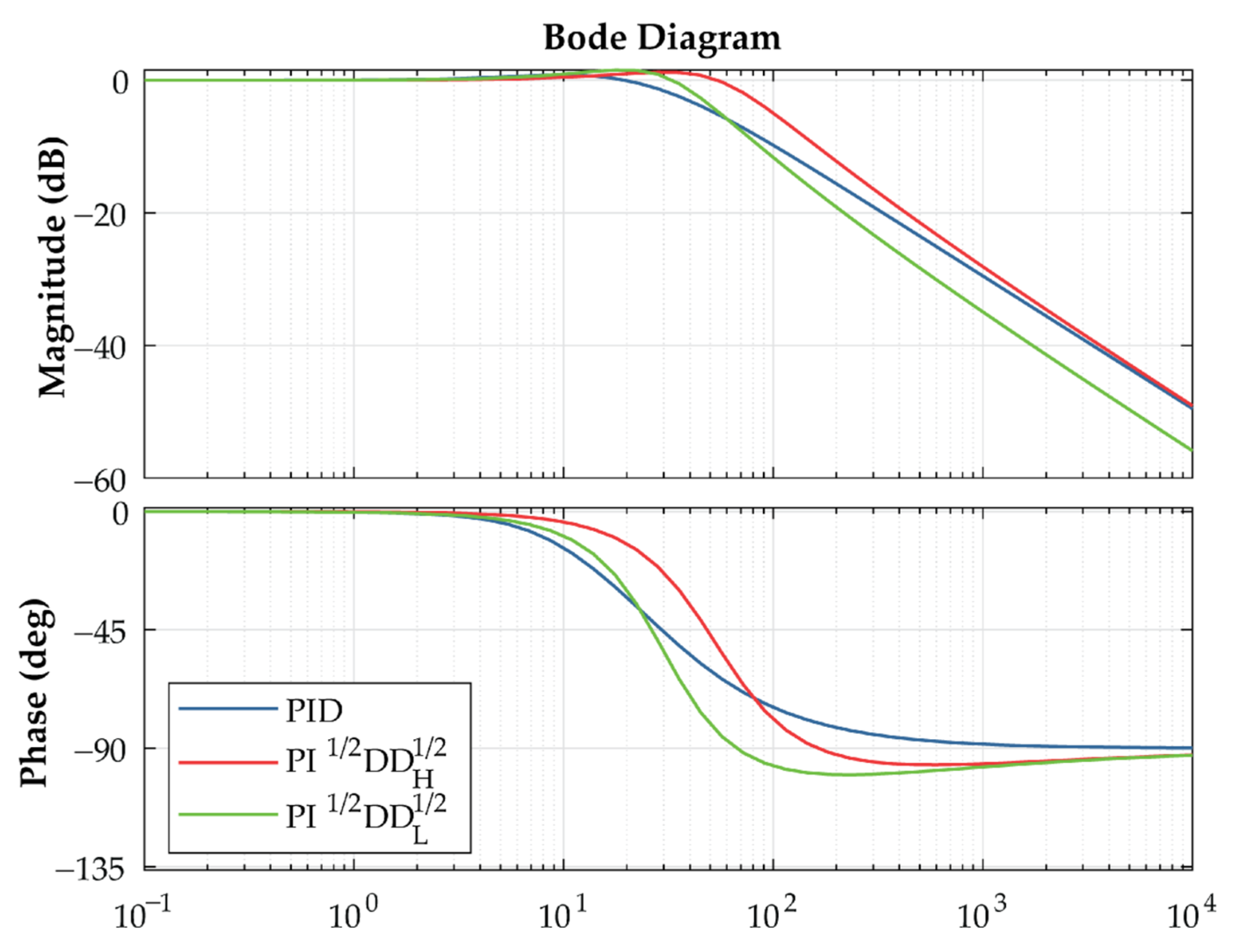
7.2. Influence of the Ratio ρ on the PII^1/2DD^1/2 Controller Frequency Response

In Section 7.1, a ratio ρ = 4 was chosen to evaluate the four corner frequencies from Equation (24). Figure 8 shows the influence of this ratio on the controller response frequency for the case study of Section 7.1. This figure shows the Bode plots of the PID controller and of the PII^1/2DD^1/2_H controllers with ρ = 1, 4, 10, 50, 200, ρ_max = 355.1. The PII^1/2DD^1/2_L controllers are not represented since the phase plot is the same and the magnitude plot is simply shifted to have the same minimum of the PID controller.

It is possible to note that:

-

the influence on the frequency response of ρ for 1 < ρ < 10 is moderate; therefore, in the example of Section 7.1, a value in the middle of this range was selected;

-

the PII^1/2DD^1/2_H with ρ = 1 does not correspond to the PID, even if its corner frequencies are paired two by two and correspond to the ones of the PID (ω’_c1 = ω’_c2 = ω_c1; ω’_c3 = ω’_c4 = ω_c2), and consequently the asymptotic bode plots are the same (the −10 dB/dec and +10 dB/dec sections have null length).

The second point may seem counterintuitive, as it comes from the fact that, as indicated by the following equation,

$$\left(1+\frac{s^{1/2}}{{\omega }_c^{1/2}}\right)\left(1+\frac{s^{1/2}}{{\omega }_c^{1/2}}\right)\ne \left(1+\frac{s}{{\omega }_c}\right)$$

(25)

two half-zero terms with the same corner frequency ω_c do not have the same transfer function and frequency response of a zero term with corner frequency ω_c, even if the asymptotic Bode plots are the same, with a change of slope from 0 dB/dec to +20 dB/dec in ω_c.

For example, Figure 9 shows the Bode plots of (i) a half-zero term with corner frequency of 100 rad/s (blue); (ii) two half-zero terms with corner frequency of 100 rad/s (red); (iii) a zero term with corner frequency of 100 rad/s (yellow). It is possible to note that the first and third plots have the same asymptotic trends for magnitude and phase, but the plot of the zero term is closer to the asymptotic plots than the one of the two half-zeros. This explains why the gain of the PII^1/2DD^1/2 with ρ = 1 is higher than the one of the PID in Figure 8.

8. Case Study: Position Control of a Rotor by PII^1/2DD^1/2 Control in Discrete Time

8.1. Digital Implementation of the PII^1/2DD^1/2 Position Control

In Section 7.1, the comparison of the controllers in the time domain (step response, Figure 7) has been carried out considering continuous-time systems (continuous-time simulation, CTS). In real applications, control algorithms are implemented digitally in discrete time with sampling time T_s; in particular, FO derivatives and integrals are evaluated by digital filters with finite memory length n by Equation (6), with T_s and n limited by the computing performance of the controller. In this section the real performance of the controllers will be compared in two steps: by carrying out simulations with discrete-time and limited memory implementations of the controllers (discrete-time simulations, DTS, Section 8.2), and by experimental tests on the physical prototype (ET, Section 8.3).

Moreover, finite displacements of position-controlled mechatronic devices are never performed using step inputs for the position set point, to avoid an abrupt increase in the error and the subsequent saturation of the control output. On the contrary, a trapezoidal speed law of the position set-point is usually adopted: a first phase with constant acceleration, then a second phase with constant speed, and finally a third phase with constant deceleration. Therefore, a trapezoidal position reference will be considered in the rest of the section.

8.2. Comparison of PID and PII^1/2DD^1/2 Controls in Discrete-Time Simulation

Let us consider the same closed-loop system discussed in Section 7.1, with the same values of J and B, and the same control gains for the three controllers (PID, PII^1/2DD^1/2_H and PII^1/2DD^1/2_L). For the discrete-time implementation of the controllers, the half-derivatives and the half-integrals are calculated by means of sixth order digital filters, according to Equation (6), adopting a sampling time T_s = 0.006 s. These values of filter order and sampling time are compatible with the computational capability of the digital controller used for the experimental validation (Section 8.3).

The considered trapezoidal position reference is characterized by: (i) a first phase with acceleration of 500 rad/s² and duration of 0.2 s, (ii) a second phase with a constant speed of 100 rad/s and duration of 0.6 s, and (iii) a third phase with deceleration of −500 rad/s² and duration of 0.2 s; consequently, the setpoint varies from 0 to 80 rad in 1 s.

The discrete-time simulations, performed by Simulink, confirm that the PII^1/2DD^1/2 controllers exhibit a better readiness than the PID control, as already shown by the continuous-time step response (Figure 7). Figure 10 represents the time histories of the angle θ, of the error e_θ and of the motor torque M. These results will be validated by experimental tests (Section 8.3) and then discussed (Section 8.4).

8.3. Comparison of PID and PII^1/2DD^1/2 Controls by Experimental Tests

The simulation results of Section 8.2 were verified by means of the experimental set-up in Figure 11a, composed of a flywheel (inertial load) directly connected to a DC motor Kollmorgen AKM42G, with maximum continuous torque of 3.4 Nm. The overall moment of inertia of the rotor, composed of the motor rotor, joint, shaft, and flywheel, is J = 1.04 × 10⁻³ kg·m². The no-load torque/speed characteristics of the rotor (i.e., the torque necessary to drive the rotor at constant speed) was measured and approximated by a linear characteristic with coefficient B = 1.45 × 10⁻³ Nms/rad. Therefore, the experimental setup is characterized by the same values of J and B considered in the simulations.

The three controllers discussed in the previous sections were implemented in Simulink Desktop Real Time running on a PC. The same Simulink model performs the DTS and the ET by means of two parallel subsystems (Figure 11b). The overall control layout is shown in Figure 12: a National Instrument PCI-6259 DAQ card, driven by Simulink Desktop Real Time, reads the encoder signal θ and generates the reference torque signal M, which is sent to a Kollmorgen driver AKD-P00606; the current reference is obtained dividing M by the torque constant k_t, and then used in the driver current loop.

Figure 13 collects the time histories of the angle θ, of the error e_θ and of the motor torque M, comparting ET (continuous lines) and DTS (dashed lines).

Table 2. Comparison of simulation results with PD, PII^1/2DD^1/2_H, and PII^1/2DD^1/2_L; for PII^1/2DD^1/2_H, and PII^1/2DD^1/2_L the variations with respect to PID are reported.

		eθ,max (rad)	eθ,mean (rad)	Mmax (Nm)	Ec (N2m2s)
PID	DTS	1.903	0.532	0.693	0.1400
	ET	1.661	0.445	0.617	0.1040
PII1/2DD1/2H	DTS	0.556	0.126	0.759	0.1437
		−70.78%	−76.32%	+9.52%	+2.61%
	ET	0.478	0.101	0.649	0.1086
		−71.22%	−77.30%	+5.19%	+4.39%
PII1/2DD1/2L	DTS	1.266	0.284	0.753	0.1545
		−33.47%	−46.62%	+8.66%	+10.30%
	ET	1.102	0.225	0.681	0.1181
		−33.65%	−49.44%	+10.37%	+13.55%

summarizes the main results in terms of maximum and mean tracking error (e_θ,max and e_θ,mean), maximum torque (M_max), and control effort (E_c): e_θ,max and is the maximum absolute value of the error, e_θ,mean is the average absolute value of the error, and E_c is defined according to the following equation:

$$E_c={\displaystyle \underset{0}{\overset{\infty }{\int }}{M}^2}dt$$

(26)

8.4. Discussion of the Results

Starting from the results presented in Section 8.2 and Section 8.3 we can draw the following conclusions:

-

The DTS and ET experimental results are in good agreement; therefore, DTS can be considered a valuable tool for the tuning of mechatronic systems with FO controllers.

-

Both the PII^1/2DD^1/2 controllers decrease the tracking error remarkably (Table 2, ET, maximum tracking error: −71% for PII^1/2DD^1/2_H and −34%for PII^1/2DD^1/2_L with respect to PID; mean tracking error: −77% for PII^1/2DD^1/2_H and −49% for PII^1/2DD^1/2_L with respect to PID), even if the increase in maximum torque and control effort is limited (ET, maximum torque: +5% for PII^1/2DD^1/2_H and +10% for PII^1/2DD^1/2_L with respect to PID; control effort: +4% for PII^1/2DD^1/2_H and +14% for PII^1/2DD^1/2_L).

-

The error reduction is higher with the tuning C_H, which is not surprising, since the gains are higher, but surprisingly the maximum torque and control effort are lower with the tuning C_H. As a matter of fact, observing the torque time histories (Figure 10 and Figure 13) it is possible to note that, with the addition of the half-order terms, the torque is delivered with lower delay even with the discrete-time calculation, consequently reducing the tracking error. This positive effect of the half-order terms is higher with the PII^1/2DD^1/2_H tuning: observing the detail zooms of Figure 13c, it is possible to notice that the torque peaks are more anticipated with the PII^1/2DD^1/2_H tuning with respect to the PII^1/2DD^1/2_L tuning.

-

This confirms the better control readiness of the PII^1/2DD^1/2 controller, already shown by the continuous-time simulations of Section 7.

9. Conclusions

In the paper, the properties of the PII^1/2DD^1/2 controller are analyzed. Then, the controller was applied to position control of a second-order plant (inertial load with viscous friction). The frequency responses of the PID, PI^λD^μ and PII^1/2DD^1/2 controllers and their asymptotic Bode plots are compared. Then, the advantages of the PII^1/2DD^1/2 controller (which is of commensurate order 1/2) over the PI^λD^μ in the stability evaluation by means of the Matignon′s theorem are highlighted.

A method for tuning the PII^1/2DD^1/2 controller is proposed. It is based on the derivation of the PII^1/2DD^1/2 asymptotic Bode plot starting from the one of a reference PID. The closed-loop frequency response, the continuous-time step response, the discrete-time simulations and the experimental tests with trapezoidal speed law demonstrate that replacement of the PID with the derived PII^1/2DD^1/2 can bring remarkable benefits in terms of system readiness and tracking error, with a limited increase in maximum torque and control effort. For the considered mechatronic axis and trapezoidal speed law, the reduction in maximum tracking error is −71% and the reduction in mean tracking error is −77% with the PII^1/2DD^1/2_H tuning, in correspondence with a limited increase in maximum torque (+5%) and control effort (+4%).

In particular, the experimental validation demonstrated that the PII^1/2DD^1/2 scheme does not require a high computational burden (the half-integral and half-derivative terms are evaluated by sixth order digital filters), and therefore can be considered as an effective and almost cost-free solution to improve the trajectory-tracking performance of position-controlled mechatronic devices, easily implementable on commercial motion control drives.

10. Related Work and Future Developments

The main limitation of this study is the lack of generality due to the fact that the performance improvement obtained by means of the PII^1/2DD^1/2 scheme with respect to PID was evaluated only for a case study with specific system parameters and starting from an arbitrary initial set of PID gains. In the work that follows, the comparison among the PID, PII^1/2DD^1/2 and PI^λD^μ controllers will be performed using a non-dimensional approach, as already done in [39] for the PD, PDD^1/2 and PD^μ controllers, without integral actions. This will provide more general results and indications on possible tuning criteria for the control of second-order linear systems, a category which may include with good approximation of many automation devices.

Moreover, in the present work only second-order plants with inertial and viscous terms and null stiffness are considered, since this linear model is adequate for most mechatronic axes; nevertheless, a possible extension is the application of the proposed control to second-order plants with non-null stiffness.

As discussed in the previous section, the proposed scheme can replace the classical PID in position control of automatic machines without significant hardware modifications; therefore, the potential field of application is very wide. In the following work, the PII^1/2DD^1/2 scheme will be applied not only to a single motor, but to more complex, multi-axis machines: CNC machine tools, industrial robots, and service robots, for example Unmanned Underwater Vehicles. For this kind of automatic vehicle, motion control strategies based on Deterministic Artificial Intelligence have been proposed [50], and a possible research direction is the application of FO algorithms in combination with these adaptive control techniques.

The discussed methodology and future directions of the work are outlined in the block diagram of Figure 14, where the green and red blocks represent, respectively, the present achievements and the prospective developments.

References

1. Miller, K.S.; Ross, B. An Introduction to the Fractional Calculus and Fractional Differential Equations; John Wiley & Sons: New York, NY, USA, 1993. [Google Scholar]
2. Das, S. Functional Fractional Calculus; Springer: Berlin/Heidelberg, Germany, 2011. [Google Scholar]
3. Sasso, M.; Palmieri, G.; Amodio, D. Application of fractional derivative models in linear viscoelastic problems. Mech. Time-Dependent Mater. 2011, 15, 367–387. [Google Scholar] [CrossRef]
4. Meral, F.C.; Royston, T.J.; Magin, R. Fractional calculus in viscoelasticity: An experimental study. Commun. Nonlinear Sci. Numer. Simul. 2010, 15, 939–945. [Google Scholar] [CrossRef]
5. Atanacković, T.M.; Pilipović, S.; Stanković, B.; Zorica, D. Fractional Calculus with Applications in Mechanics: Wave Propagation, Impact and Variational Principles; Wiley: New Jersey, NY, USA, 2014. [Google Scholar]
6. Hilfer, R. Applications of Fractional Calculus in Physics; World Scientific: Singapore, 2000. [Google Scholar]
7. Rihan, F.A. Numerical Modeling of Fractional-Order Biological Systems. Abstr. Appl. Anal. 2013, 2013, 816803. [Google Scholar] [CrossRef] [Green Version]
8. Shaikh, A.S.; Shaikh, I.N.; Nisar, K.S. A mathematical model of COVID-19 using fractional derivative: Outbreak in India with dynamics of transmission and control. Adv. Differ. Equ. 2020, 2020, 373. [Google Scholar] [CrossRef] [PubMed]
9. Kozioł, K.; Stanisławski, R.; Bialic, G. Fractional-Order SIR Epidemic Model for Transmission Prediction of COVID-19 Disease. Appl. Sci. 2020, 10, 8316. [Google Scholar] [CrossRef]
10. Podlubny, I. Fractional-order systems and PIλDμ controllers. IEEE Trans. Autom. Control. 1999, 44, 208–213. [Google Scholar] [CrossRef]
11. Yeroglu, C.; Tan, N. Note on fractional-order proportional-integral-differential controller design. IET Control. Theory Appl. 2012, 5, 1978–1989. [Google Scholar] [CrossRef]
12. Beschi, M.; Padula, F.; Visioli, A. The generalised isodamping approach for robust fractional PID controllers design. Int. J. Control. 2015, 90, 1157–1164. [Google Scholar] [CrossRef]
13. Kesarkar, A.A.; Selvaganesan, N. Tuning of optimal fractional-order PID controller using an artificial bee colony algorithm. Syst. Sci. Control. Eng. 2015, 3, 99–105. [Google Scholar] [CrossRef] [Green Version]
14. Norsahperi, N.M.H.; Danapalasingam, K.A. Particle swarm-based and neuro-based FOPID controllers for a Twin Rotor System with improved tracking performance and energy reduction. ISA Trans. 2020, 102, 230–244. [Google Scholar] [CrossRef]
15. Saidi, B.; Amairi, M.; Najar, S.; Aoun, M. Bode shaping-based design methods of a fractional order PID controller for uncertain systems. Nonlinear Dyn. 2015, 80, 1817–1838. [Google Scholar] [CrossRef]
16. Oshnoei, A.; Khezri, R.; Muyeen, S.M.; Blaabjerg, F. On the Contribution of Wind Farms in Automatic Generation Control: Review and New Control Approach. Appl. Sci. 2018, 8, 1848. [Google Scholar] [CrossRef] [Green Version]
17. Anantachaisilp, P.; Lin, Z. Fractional Order PID control of rotor suspension by active magnetic bearings. Actuators 2017, 6, 4. [Google Scholar] [CrossRef] [Green Version]
18. Sondhi, S.; Hote, Y.V. Fractional order PID controller for perturbed load frequency control using Kharitonov’s theorem. Electr. Power Energy Syst. 2016, 78, 884–896. [Google Scholar] [CrossRef]
19. Yang, B.; Wang, J.; Wang, J.; Shu, H.; Li, D.; Zeng, C.; Chen, Y.; Zhang, X.; Yu, T. Robust fractional-order PID control of supercapacitor energy storage systems for distribution network applications: A perturbation compensation based approach. J. Clean. Prod. 2021, 279, 123362. [Google Scholar] [CrossRef]
20. Khubalkar, S.; Chopade, A.; Junghare, A.; Aware, M.; Das, S. Design and realization of stand-alone digital Fractional Order PID controller for buck converter fed DC Motor. Circuits Syst. Signal. Process. 2016, 35, 2189–2211. [Google Scholar] [CrossRef]
21. Dimeas, I.; Petras, I.; Psychalinos, C. New analog implementation technique for fractional-order controller: A DC motor control. AEU Int. J. Electron. Commun. 2017, 78, 192–200. [Google Scholar] [CrossRef]
22. Haji, V.; Monje, C. Fractional-order PID control of a chopper-fed DC motor drive using a novel firefly algorithm with dynamic control mechanism. Soft Comput. 2018, 22, 6135–6146. [Google Scholar] [CrossRef]
23. Hekimoglu, B. Optimal Tuning of Fractional Order PID Controller for DC Motor Speed Control via Chaotic Atom Search Optimization Algorithm. IEEE Access 2019, 7, 38100–38114. [Google Scholar] [CrossRef]
24. Puangdownreong, D. Fractional order PID controller design for DC motor speed control system via flower pollination algorithm. Trans. Electr. Eng. Electron. Commun. 2019, 17, 14–23. [Google Scholar] [CrossRef]
25. Viola, J.; Angel, L.; Sebastian, J.M. Design and robust performance evaluation of a Fractional Order PID controller applied to a DC Motor. IEEE/CAA J. Autom. Sin. 2017, 4, 304–314. [Google Scholar] [CrossRef]
26. Olejnik, P.; Adamski, P.; Batory, D.; Awrejcewicz, J. Adaptive Tracking PID and FOPID Speed Control of an Elastically Attached Load Driven by a DC Motor at Almost Step Disturbance of Loading Torque and Parametric Excitation. Appl. Sci. 2021, 11, 679. [Google Scholar] [CrossRef]
27. Zheng, W.; Luo, Y.; Pi, Y.; Chen, Y. Improved frequency-domain design method for the fractional order proportional-integral-derivative controller optimal design: A case study of permanent magnet synchronous motor speed control. IET Control. Theory Appl. 2018, 12, 2478–2487. [Google Scholar] [CrossRef]
28. Sun, G.; Ma, Z.; Yu, J. Discrete-Time Fractional Order Terminal Sliding Mode Tracking Control for Linear Motor. IEEE Trans. Ind. Electron. 2018, 65, 3386–3394. [Google Scholar] [CrossRef]
29. Chen, S.Y.; Li, T.H.; Chang, C.H. Intelligent fractional-order backstepping control for an ironless linear synchronous motor with uncertain nonlinear dynamics. ISA Trans. 2019, 89, 218–232. [Google Scholar] [CrossRef]
30. Lino, P.; Maione, G. Cascade Fractional-Order PI Control of a Linear Positioning System. IFAC PapersOnLine 2018, 51, 557–562. [Google Scholar] [CrossRef]
31. Wang, Z.; Wang, X.; Xia, J.; Shen, H.; Meng, B. Adaptive sliding mode output tracking control based-FODOB for a class of uncertain fractional-order nonlinear time-delayed systems. Sci. China Technol. Sci. 2020, 63, 1854–1862. [Google Scholar] [CrossRef]
32. Han, S. Grey Wolf and Weighted Whale Algorithm Optimized IT2 Fuzzy Sliding Mode Backstepping Control with Fractional-Order Command Filter for a Nonlinear Dynamic System. Appl. Sci. 2021, 11, 489. [Google Scholar] [CrossRef]
33. Bruzzone, L.; Bozzini, G. Application of the PDD1/2 algorithm to position control of serial robots. In Proceedings of the 28th IASTED International Conference Modelling, Identification and Control (MIC 2009), Innsbruck, Austria, 16–18 February 2009; pp. 225–230. [Google Scholar]
34. Bruzzone, L.; Bozzini, G. PDD1/2 control of purely inertial systems: Nondimensional analysis of the ramp response. In Proceedings of the 30th IASTED International Conference Modelling, Identification, and Control (MIC 2011), Innsbruck, Austria, 14–16 February 2011; pp. 308–315. [Google Scholar] [CrossRef]
35. Bruzzone, L.; Fanghella, P. Fractional order control of the 3-CPU parallel kinematics Machine. In Proceedings of the 32nd IASTED International Conference Modelling, Identification and Control (MIC 2013), Innsbruck, Austria, 11–13 February 2013; pp. 286–292. [Google Scholar] [CrossRef]
36. Bruzzone, L.; Fanghella, P. Fractional-order control of a micrometric linear axis. J. Control. Sci. Eng. 2013, 2013, 947428. [Google Scholar] [CrossRef] [Green Version]
37. Corinaldi, D.; Palpacelli, M.; Carbonari, L.; Bruzzone, L.; Palmieri, G. Experimental analysis of a fractional-order control applied to a second order linear system. In Proceedings of the 10th IEEE/ASME International Conference on Mechatronic and Embedded Systems and Applications (MESA 2014), Senigallia, Italy, 10–12 September 2014; p. 108901. [Google Scholar] [CrossRef]
38. Bruzzone, L.; Fanghella, P. Comparison of PDD1/2 and PDμ position controls of a second order linear system. In Proceedings of the 33rd IASTED International Conference on Modelling, Identification and Control (MIC 2014), Innsbruck, Austria, 17–19 February 2014; pp. 182–188. [Google Scholar] [CrossRef]
39. Bruzzone, L.; Fanghella, P.; Baggetta, M. Experimental assessment of Fractional-Order PDD1/2 control of a brushless DC motor with inertial load. Actuators 2020, 9, 13. [Google Scholar] [CrossRef] [Green Version]
40. Bruzzone, L.E.; Molfino, R.M.; Zoppi, M. An impedance-controlled parallel robot for high-speed assembly of white goods. Ind. Robot. 2005, 32, 226–233. [Google Scholar] [CrossRef]
41. Jakovljevic, B.B.; Sekara, T.B.; Rapaic, M.R.; Jelicic, Z.D. On the distributed order PID controller. Int. J. Electron. Commun. 2017, 79, 94–101. [Google Scholar] [CrossRef]
42. Jakovljevic, B.B.; Lino, P.; Maione, G. Fractional and Distributed Order PID Controllers for PMSM Drives. In Proceedings of the 18th European Control Conference (ECC), Napoli, Italy, 25–28 June 2019; pp. 4100–4105. [Google Scholar]
43. Jakovljevic, B.B.; Lino, P.; Maione, G. Control of double-loop permanent magnet synchronous motor drives by optimized fractional and distributed-order PID controllers. Eur. J. Control 2021, 58, 232–244. [Google Scholar] [CrossRef]
44. Podlubny, I. Fractional Differential Equations; Academic Press: New York, NY, USA, 1999. [Google Scholar]
45. Machado, J.T. Fractional-order derivative approximations in discrete-time control systems. J. Syst. Anal. Model. Simul. 1999, 34, 419–434. [Google Scholar]
46. Chen, Y.Q.; Petras, I.; Xue, D. Fractional Order Control—A Tutorial. In Proceedings of the 2009 American Control Conference, St. Louis, MO, USA, 10–12 June 2009; pp. 1397–1411. [Google Scholar]
47. Monje, C.A.; Chen, Y.Q.; Vinagre, B.M.; Xue, D.; Feliu, V. Fractional-Order Systems and Controls; Springer: London, UK, 2010. [Google Scholar]
48. Matignon, D. Generalized Fractional Differential and Difference Equations: Stability Properties and Modelling Issues. In Proceedings of the Mathematical Theory of Networks and Systems Symposium, Padova, Italy, 6–10 July 1998. [Google Scholar]
49. Tavazoei, M.; Asemani, M.H. On robust stability of incommensurate fractional-order systems. Commun. Nonlinear Sci. Numer. Simulat. 2020, 90, 105344. [Google Scholar] [CrossRef]
50. Sands, T. Control of DC Motors to Guide Unmanned Underwater Vehicles. Appl. Sci. 2021, 11, 2144. [Google Scholar] [CrossRef]
Figure 1. Closed-loop system with a second-order plant.
Applsci 11 03631 g001
Figure 2. Example frequency responses of PID (blue), PIλDμ (yellow) and PII1/2DD1/2 (red) controllers.
Applsci 11 03631 g002
Figure 3. Stability regions of fractional order systems with fractional commensurate order q = 1/2.
Applsci 11 03631 g003
Figure 4. Derivation of the PII1/2DD1/2 control parameters from the PID control Bode plot: PID (blue); PII1/2DD1/2 with tuning CH (red); PII1/2DD1/2 with tuning CL (green).
Applsci 11 03631 g004
Figure 5. Comparison of the controller Bode plots: PID (blue); PII1/2DD1/2H (red); PII1/2DD1/2L (green); the phase plots of the two PII1/2DD1/2 controllers are equal.
Applsci 11 03631 g005
Figure 6. Comparison of the closed-loop system Bode plots: PID (blue); PII1/2DD1/2H (red); PII1/2DD1/2L (green).
Applsci 11 03631 g006
Figure 7. Comparison of the unit step responses of the closed-loop systems: PID (blue); PII1/2DD1/2H (red); PII1/2DD1/2L (green).
Applsci 11 03631 g007
Figure 8. Influence of the ratio ρ of the controller Bode plots: PID (blue) and PII1/2DD1/2H (red), for ρ = 1, 4, 10, 50, 200, ρmax = 355.1.
Applsci 11 03631 g008
Figure 9. Bode plots of: a half-zero term with corner frequency of 100 rad/s (blue); two half-zero terms with corner frequency of 100 rad/s (red); a zero term with corner frequency of 100 rad/s (yellow).
Applsci 11 03631 g009
Figure 10. Trapezoidal speed law response, discrete-time simulation: angle θ (a), error eθ (b) and motor torque M (c); PID: blue; PII1/2DD1/2H: red; PII1/2DD1/2L: green; set-point: black.
Applsci 11 03631 g010
Figure 11. Experimental layout: flywheel directly actuated by the brushless DC motor (a) and Simulink Desktop Real Time control scheme (b).
Applsci 11 03631 g011
Figure 12. Overall control scheme of the experimental layout.
Applsci 11 03631 g012
Figure 13. Trapezoidal speed law response, comparison of ET (continuous line) and DTS (dashed line): angle θ (a), error eθ (b) and motor torque M (c); PID: blue; PII1/2DD1/2H: red; PII1/2DD1/2L: green; set-point: black.
Applsci 11 03631 g013
Figure 14. Block diagram of the research methodology and future research directions (green blocks: present achievements; red blocks: prospective developments).
Applsci 11 03631 g014