Optimization of Well Placement in Carbon Capture and Storage (CCS): Bayesian Optimization Framework under Permutation Invariance

Abstract

Carbon Capture and Storage (CCS) stands as a pivotal technological stride toward a sustainable future, with the practice of injecting supercritical CO₂ into subsurface formations being already an established practice for enhanced oil recovery operations. The overarching objective of CCS is to protract the operational viability and sustainability of platforms and oilfields, thereby facilitating a seamless transition towards sustainable practices. This study introduces a comprehensive framework for optimizing well placement in CCS operations, employing a derivative-free method known as Bayesian Optimization. The development plan is tailored for scenarios featuring aquifers devoid of flow boundaries, incorporating production wells tasked with controlling pressure buildup and injection wells dedicated to CO₂ sequestration. Notably, the wells operate under group control, signifying predefined injection and production targets and constraints that must be adhered to throughout the project’s lifespan. As a result, the objective function remains invariant under specific permutations of the well locations. Our investigation delves into the efficacy of Bayesian Optimization under the introduced permutation invariance. The results reveal that it demonstrates critical efficiency in handling the optimization task extremely fast. In essence, this study advocates for the efficacy of Bayesian Optimization in the context of optimizing well placement for CCS operations, emphasizing its potential as a preferred methodology for enhancing sustainability in the energy sector.

1. Introduction

In recent years, the discourse surrounding climate change has intensified, with a growing consensus on the imperative need to transition the global economy towards achieving net-zero greenhouse gas emissions by mid-century. This ambitious goal, essential to averting dangerous anthropogenic interference with the climate system, requires rapid investment increase in near-zero emission technologies across all sectors [1]. Among these technologies, Carbon Capture and Storage (CCS), also referred to as CCUS, where “U” stands for utilization, shows to be a pivotal solution to reducing carbon emissions, addressing climate change, and facilitating the transition to a carbon-neutral future [2,3]. Its significance lies in its potential to address emissions from various sources, including power-generating plants, hard-to-abate industries (such as cement and refineries), and hydrogen production. CCUS is the only technology capable of guiding industries to absolute net neutrality by capturing and treating emissions.

Once CO₂ is captured, it undergoes compression and transport to be permanently stored in geological formations, acting as a “sink” through injection. These geological formations must possess certain key characteristics [4]. Essential conditions for a formation to be considered a suitable carbon storage site include the formation of a pore unit with sufficient capacity to store the intended CO₂ volume; pore interconnectivity allowing injection at the required rate; and the presence of an extensive cap rock or barrier at the top of the formation to retain the injected CO₂, prevent unwanted migration, and ensure long-term containment [5]. Saline water-bearing formations [6,7,8] are widely regarded as the most mature options for CO₂ storage, as demonstrated by numerous projects worldwide. Additionally, depleted oil and gas fields have recently emerged as potential storage sites, benefitting from operational experience gained through CO₂-EOR operations [9,10,11].

Deploying CCUS technology on a large scale in saline aquifers or hydrocarbon fields necessitates accurate characterization of the storage site and reservoir, involving a complex process, from screening to deep geological and geophysical characterization [12]. Numerical simulation and modeling using computational fluid dynamics (CFD), possibly coupled with reactive transport simulations, are employed to address complex subsurface geology, simulating the flow behavior of the injected and the in situ fluids. The goal of such models is to estimate the field sequestration capacity of the injected CO₂ under different trapping mechanisms, such as structural, dissolution, residual, and mineral storage, during all project phases [13,14].

Reservoir simulation is a crucial tool in the field of petroleum engineering that aids in modeling and predicting fluid flow behavior within subsurface reservoirs. The primary objective is to simulate the complex interactions among various components, such as rock, fluids, and wells. One of the fundamental principles underlying reservoir simulation is Darcy’s law, which describes the flow of fluids through porous media. The Darcy equation (Equation (1)) relates fluid velocity to pressure gradient, permeability, and fluid viscosity [15]. The simulator employs numerical methods to solve the mass, momentum, and energy differential equations governing fluid flow (2) in the porous medium. The most widely used flow model in reservoir simulation is the black-oil one [16]. In the black-oil formulation [17], the model is considered to consist of three separate fluid phases or pseudocomponents (water, oil, and gas). Mixing among phases is allowed, and the amount of how much each phase is dissolved in the others and how it affects flow properties need to be kept tracked of.

$${\mathbf{v}}_a=-{\lambda }_a\mathbf{K}(\nabla p_a-{\rho }_a\mathbf{g})$$

(1)

$$\frac{\partial }{\partial t}\left(\varphi A_a\right)+\nabla {\mathbf{u}}_a+q_a=0$$

(2)

where the subscript a denotes the pseudocomponent oil (o), gas (g), or water (w). For each one, the variables are defined as follows: ${\mathbf{v}}_a$ is the phase flux, and ${\lambda }_a$ is the mobility of the phase. This is defined as ${\lambda }_a=\frac{k_{r,a}}{{\mu }_a}$, where ${\mu }_a$ and $k_{r,a}$ are the viscosity and the relative permeability of each phase, respectively. In short, relative permeability is a measure of the effective permeability reduction of a phase in the presence of other phases and is a function of saturation. $p_a$ is the pressure, ${\rho }_a$ is the density, and $q_a$ is the well outflux/influx of each phase, i.e., the volumetric flow rate at which each pseudocomponent is produced/injected from the system. $A_a=f(b_w,b_o,b_g,s_w,s_o,s_g)$ are accumulation terms dependent on phase saturation ($s_a$) and shrinkage phase factors ($b_a$). The flux terms ${\mathbf{u}}_a=f({\mathbf{v}}_w,{\mathbf{v}}_o,{\mathbf{v}}_g,b_w,b_o,b_g)$ are known functions of shrinkage factor and phase fluxes. Finally, the terms $\varphi$ and $\mathbf{K}$ are the porosity and permeability, respectively.

The other popular simulation model is the compositional one [18,19]. The difference between the black-oil and compositional models lies in that the former traces the flow of each separate phase; hence, it only considers single-phase (gas, oil, and water) density and compressibility effects, as well as dissolution of gas in the oil phase. The fact that the volumetric and dissolution factors can be easily described by simple functions of the pressure is based on the assumption that the overall composition does not change significantly during reservoir depletion or waterflooding. On the other hand, compositional modeling, facilitated by means of an EoS model, is used when some “alien” composition is incorporated in the reservoir fluids. This is the typical case when handling EOR cases of CO₂, natural or acid gas injection, and injection of dry gas in gas condensate reservoirs.

Equations (1) and (2) are combined in a second-order partial differential equation (PDE) which can be analytically solved under simplifying assumptions (incompressible, single-phase system with constant porosity and permeability). However, when trying to model realistic subsurface formations, these assumptions do not hold. In this case, the discretization of the equation through linearization is a key step in numerical reservoir simulation. This process involves dividing the reservoir into a grid to represent the spatial distribution of rock properties and fluid flow and using a linearization scheme [20]. Common methods for discretization include finite differences, finite volumes, and finite elements. Finite volumes [21], in particular, are widely used in reservoir simulation due to their simplicity and efficiency. Gridding plays a vital role in the discretization process, involving defining the size and shape of the cells within the reservoir grid. Various types of grids, such as Cartesian, corner-point, and unstructured grids, are used based on the geological complexity of the reservoir. The choice of grid impacts the accuracy and computational efficiency of the simulation.

Petrophysical and fluid properties, such as porosity, permeability, fluid saturation, compressibility, and relative permeability, are crucial inputs for reservoir simulation [22,23]. Accurate characterization of these properties is essential for realistic simulation results. Furthermore, incorporating phase behavior models is essential to accurately representing the complex interactions among different phases of fluids and dissolved particles in multi-phase flow simulations. For instance, in CCS simulations, it is crucial to capture the dynamics of CO₂ dissolution, which significantly depends on the concentration of salts in the aquifer [24].

Building upon the foundation of accurate simulation models, the optimization of well placement becomes paramount to maximizing the sequestration potential of the aquifer in CCS endeavors [25,26]. The primary objective of CCS projects is to maximize CO₂ storage while adhering to constraints and technical policies [27,28]. In its most commonly employed form, the CCS plan requires that brine producers be closed off once significant CO₂ breakthrough occurs, whereas the injectors rate is reduced when the bottomhole pressure reaches the safety limit. Consequently, optimal well placement significantly influences the overall success of the sequestration project by delaying the breakthrough time. The objective function maximization in this context is defined as achieving the highest attainable CO₂ storage, considering the spatial distribution of the injection and brine withdrawal wells. This multi-dimensional function has an unknown functional form and its point values are expensive to compute since each one requires a fully implicit simulation to be run. Therefore, it needs to be treated as a black-box function.

Well placement decisions cannot rely solely on static properties, since geological variables are mostly non-linearly correlated to production performance. This is demonstrated in Figure 1, where the objective function of oil production in the form of the expected net present value (NPV) is evaluated for the placement of a single oil producer in each cell. The complexity and non-linearity in CCS projects parallel those encountered in oil production, underscoring the importance of optimized well placement for maximizing storage efficiency while considering factors such as CO₂ dissolution dynamics and aquifer characteristics. In general, well placement optimization poses a formidable challenge due to the large number of the decision variables involved, the high non-linearity of the system response, the abundance of local optima, and the well placement constraints. Due to the discontinuities and the inherent non-smoothness of the objective, research has been mostly focused on derivative-free optimization methods such as Genetic Algorithms [29] and Particle Swarm Optimization [30] combined with various heuristics.

Guyaguler et al. (2002) [31] developed and applied the Hybrid Genetic Algorithm (HGA) [32] to determine the optimal location and number of vertical wells, while Badru et al. (2003) [33] extended this work to also include horizontal wells. In essence, HGA comprises Genetic Algorithm (GA), the polytope algorithm for selecting the fittest individuals and a kriging proxy to expedite the optimization process. The results showed that after a few simulation runs, the method was able to optimize the production’s NPV compared with the base case. In another work, Emerick et al. (2009) [34] designed a tool for well placement optimization using a GA with non-linear constraints. They applied the GENOCOP III algorithm [35] which utilizes two separate populations where the evolution in one influences the evaluation of the other. The first population, named the “search population”, consists of individuals that satisfy the linear constraints, whereas the second, called the “reference population”, consists only of those that satisfy both linear and non-linear constraints. By using this procedure, the research team developed a tool that handled a total of eight decision variables per well (six in total that define the heel and toe coordinates of the well, one binary for producer or injector, and one defining active or inactive well). The results showed a significant increase in the NPV of the production plan in comparison with the base case proposed plans. Stopa et al. (2016) [36] applied both GA and PSO to optimize well placement and well rates. Their approach was different in that they utilized an objective function that measures the ratio of the volume of mobile CO₂ phase (plume) over the volume of CO₂ injected after 10 years of injection and 80 years of monitoring. Their goal was to minimize this ratio, since by minimizing the plume, leakage risk is also reduced. In essence, they tried to find configurations that maximized the residual and solubility trapping of CO₂. In their work, PSO was able to find the optimal value of 12.5% in 500 simulation runs, while GA needed more than 850. Similarly, Goda and Sato (2013) [37] utilized a similar objective function by using a global sampling method known as Latin Hypercube Sampling (LHS) [38]. Notably, in their work, they enhanced the definition of immobile CO₂ by taking into account the irreducibility of relative permeability curves. Besides the mentioned landmark works, there have been dozens more published on this optimization problem. Islam et al. (2020) [39] provided a detailed review of research conducted on the well placement optimization problem, focusing mostly on derivative-free and machine learning regression methods.

Bayesian Optimization (BO) [40] is a global optimization method that efficiently constructs and updates surrogate models representing black-box objective functions, rendering it suitable for addressing the well placement optimization problem. In this work, our goal is to apply this method to optimize the carbon sequestration capabilities of a saline aquifer. BO represents a cutting-edge methodology that dynamically balances the exploration of the solution space with the exploitation of promising regions to efficiently discover well placement that can lead to the global optimum configuration. BO relies on constructing a probabilistic surrogate model, often a Gaussian Process (GP), to approximate the underlying objective function, which, in this context, measures total carbon storage. This surrogate model not only captures the observed data but also quantifies the uncertainty associated with predictions, allowing for the incorporation of prior knowledge and continuous refinement as new information becomes available through successive simulation runs. By iteratively selecting well locations based on the surrogate model’s predictions and subsequently updating the model with the actual reservoir response, BO intelligently adapts its search strategy. This adaptive nature makes it particularly well suited for navigating the high-dimensional and uncertain parameter space, providing a systematic and data-driven means of identifying optimal well configurations for enhanced carbon sequestration.

BO for well placement optimization was implemented in the work of Balabaeva et al. (2020) [41]. In their work, the researchers attempted to optimize well locations by maximizing the cumulative drainage area of wells by using various derivative-free methods, with BO being one of them. In another work, Bordas et al. (2020) [42] utilized a BO framework for field development planning while quantifying the effect of geological uncertainty. They generated a surrogate model that was able to identify well placement positions that maximized NPV while accounting for uncertainty. Kumar [43,44] also presented works on novel BO realizations, such as trust region BO [45] and sparse-axis-aligned subspaces BO (SAASBO) [46]. BO has additionally been investigated for optimizing various decision variables crucial in reservoir exploitation besides well placement. Lu et al. (2022) [47] utilized BO to optimize the time cycle of gas/surfactant injection in Water Alternating Gas (WAG) schemes. Their study conducted at the Cranfield reservoir site resulted in a 16% increase in gas storage volume and a 56% reduction in water/surfactant usage compared with the baseline WAG schedule. In an MSc thesis, Javed [48] employed a BO framework to optimize deviated well trajectories in a synthetic reservoir model located in the North Sea. The optimized trajectories led to a 28% enhancement in the objective function compared with the base case. Additionally, Wang and Chen (2017) [49] investigated the Cardium tight formation, where they successfully optimized fracturing design parameters by using BO, achieving a notable 55% improvement in the objective function. These studies prove BO to be a suitable framework in reservoir engineering. However, to our knowledge, BO has not been studied for the well placement optimization problem in CCS specifically.

The rest of the paper is organized as follows: In Section 2, we delve into a comprehensive explanation of the Bayesian Optimization method. Following that, Section 3 offers a detailed description of the specific problem, elucidating how BO was strategically applied to address the challenges encountered, such as non-linear constraints and permutation invariance in the input space. In Section 4, we present results stemming from various implementations of the BO method, comparing the performance of various acquisition functions and inspecting the exploration–exploitation trade-off. Section 5 initiates an expansive discussion of the obtained results. Finally, Section 6 draws insightful conclusions based on the findings and discussions presented throughout the study.

Figure 1. NPV evaluation for oil production with a single well [50].

Figure 1. NPV evaluation for oil production with a single well [50].

2. Bayesian Optimization

2.1. Gaussian Process (GP) Regression

In order to properly understand BO, the GP framework needs to be explained in detail. The complete treatment of GP can be found in Rasmussen and Williams (2006) [51]. Most of the material in this section has been inspired by Frazier (2018) [40] and Dou (2015) [52] and the articles by Distill [53,54], which provide visual and interactive explanations of the materials discussed here.

Multivariate Gaussian distributions (MVN) [55] act as the building blocks of GP. They express the distribution of multiple random variables that are distributed normally and whose joint distribution is also Gaussian. They are defined by a mean vector $\mathbf{\mu }$, which describes the expected value of the distribution, and a positive semidefinite covariance matrix Σ, which models the variance along each dimension and determines how the different random variables are correlated. The diagonal elements of Σ express the variance of each random variable. The off-diagonal elements ${\Sigma }_{i,j}$ describe the correlation between the ith and jth random variables. The probability density of an MVN in d dimensions is shown in Equation (3).

$$N\left(\mathbf{x}\right|\mathbf{\mu },\mathbf{\Sigma })={\displaystyle \frac{1}{{\left(2\pi \right)}^{d/2}{\left|\mathbf{\Sigma }\right|}^{1/2}}}exp\left[-\frac{1}{2}{(\mathbf{x}-\mathbf{\mu })}^T{\mathbf{\Sigma }}^{-1}(\mathbf{x}-\mathbf{\mu })\right]$$

(3)

where $\mathbf{\mu }$ is the $d\times 1$ mean vector and Σ is the $d\times d$ covariance matrix. A GP is the extension of this MVN to the space of functions, defining a probability measure on a function space. This function space acts as the probabilistic surrogate objective function, which will eventually converge to the actual objective function through sampling and utilization of the GP regression algorithm. At first, the probability measure is interpreted as our prior knowledge about the unknown objective function before data are seen. A GP is defined via its mean and covariance just like the MVN; however, those now represent functions. Given a finite collection of q points ${\mathbf{x}}_{1:q}\in {\mathbb{R}}^d$ that appropriately discretize the d-dimensional input space, the objective function’s values $\mathbf{f}\left({\mathbf{x}}_{1:q}\right)$ are assumed to be drawn by an MVN.

$$\mathbf{f}\left({\mathbf{x}}_{1:q}\right)\sim N(\mathbf{m}\left({\mathbf{x}}_{1:q}\right),\mathbf{K}({\mathbf{x}}_{1:q},{\mathbf{x}}_{1:q}))$$

(4)

Compared with a multivariate normal, we have the following:

• A random function vector $\mathbf{f}(·)$ instead of a random vector $\mathbf{x}$;
• A mean function vector $\mathbf{m}(·)$ instead of a mean vector $\mathbf{\mu }$;
• A covariance (kernel) function matrix $\mathbf{K}(·,·)$ instead of a covariance matrix Σ.

Above, $\mathbf{K}(·,·)=\left\{k({\mathbf{x}}_i,{\mathbf{x}}_j)\right\}$ and $k({\mathbf{x}}_i,{\mathbf{x}}_j)$ is the kernel function discussed below.

Equation (4) states that the vector of functions conditional on inputs ${\mathbf{x}}_{1:q}$ and the mean and covariance functions follows a q-dimensional MVN distribution. To avoid confusion, it needs to be stated that no assumption has been made on the distribution of the inputs. So far, the prior Gaussian distribution of the objective function has been defined. Function values selected in the prior are commonly referred to in the literature as the test data.

In the prior distribution, it is common to set the mean function to a constant value of zero. This is a reasonable assumption since no prior knowledge is assumed. If prior knowledge can be assumed to exist, then the mean function can be set to Equation (5).

$$m\left(\mathbf{x}\right)={\mu }_0+\sum _{i=1}^p{\beta }_i{\Psi }_i\left(\mathbf{x}\right)$$

(5)

where ${\Psi }_i$ are often parametric, low-order polynomials which summarize our prior knowledge on the objective function.

When it comes to choosing a kernel function, it is typically necessary to select it based on certain properties. First of all, kernel functions need to be positive semidefinite. Secondly, it is important that points closer in the input space are more strongly correlated, i.e., if $\left|\right|\mathbf{x}-{\mathbf{x}}^{\prime }\left|\right|<\left|\right|\mathbf{x}-{\mathbf{x}}^{″}\left|\right|$, then $k(\mathbf{x},{\mathbf{x}}^{\prime })>k(\mathbf{x},{\mathbf{x}}^{″})$. There are many kernel functions commonly used in BO; however, the Matérn kernel [56] will be the main focus, since it is a more general form of kernel functions.

$$k(\mathbf{x},{\mathbf{x}}^{\prime })={\alpha }_0{\displaystyle \frac{2^{1-\nu }}{\Gamma \left(\nu \right)}}{\left(\sqrt{2\nu }\left|\right|\mathbf{x}-{\mathbf{x}}^{\prime }\left|\right|\right)}^{\nu }{K}_{\nu }(\sqrt{2\nu }\left|\right|\mathbf{x}-{\mathbf{x}}^{\prime }\left|\right|)$$

(6)

where $K_{\nu }$ is the modified Bessel function [57], $\Gamma \left(\nu \right)$ is the Gamma function, and ${\alpha }_0$ is a hyperparamter [58]. Certain values of $\nu$ in Equation (6) reduce the equation to other popular kernels, including the following:

• Radial basis function (RBF) kernel [59] for $\nu \to inf$;
• Absolute exponential kernel for $\nu =0.5$;
• Once-differentiable functions for $\nu =1.5$;
• Twice-differentiable functions for $\nu =2.5$.

So far, the prior distribution of functions has been constructed, but no observed information has been introduced to the model yet. To do so, the objective function’s value has to be measured at some points, which are denoted by ${\mathbf{y}}_{1:n}$. These points, commonly referred to as training data, are observed by sampling the black-box objective function. By incorporating this information into our model, the posterior distribution can be defined. First of all, the distribution of $\mathbf{f}({\mathbf{x}}_{1:q},{\mathbf{y}}_{1:n})$ is now a $(q+n)$-dimensional MVN. To acquire the posterior distribution on a certain point of ${\mathbf{x}}_{1:q}$, conditioning and marginalization have to be applied. By using the Bayes rule, Equation (7) is obtained.

$$f\left(\mathbf{x}\right)|\mathbf{f}\left({\mathbf{y}}_{1:n}\right)\sim N({\mu }_n\left(\mathbf{x}\right),{\sigma }_n^2\left(\mathbf{x}\right))$$

(7)

where the mean value ${\mu }_n\left(\mathbf{x}\right)$ is given by Equation (8) and represents a weighted average between the prior and an estimate based on the training data.

$${\mu }_n\left(\mathbf{x}\right)=\mathbf{k}(\mathbf{x},{\mathbf{y}}_{1:n})\mathbf{K}{({\mathbf{y}}_{1:n},{\mathbf{y}}_{1:n})}^{-1}\left(\mathbf{f}\left({\mathbf{y}}_{1:n}\right)-{\mathbf{\mu }}_0\left({\mathbf{y}}_{1:n}\right)\right)+{\mu }_0\left(\mathbf{x}\right)$$

(8)

and the posterior variance ${\sigma }_n^2\left(\mathbf{x}\right)$ seen in Equation (9) is equal to the previous covariance, minus a term that corresponds to the variance removed by observing the training data.

$${\sigma }_n^2\left(\mathbf{x}\right)=k(\mathbf{x},\mathbf{x})-\mathbf{k}(\mathbf{x},{\mathbf{y}}_{1:n})\mathbf{K}{({\mathbf{y}}_{1:n},{\mathbf{y}}_{1:n})}^{-1}\mathbf{k}({\mathbf{y}}_{1:n},\mathbf{x})$$

(9)

This regression process updates the surrogate objective function’s values by conditioning on the training data.

2.2. Kernel Functions

Kernel functions are essential in BO since they define the shape of the prior and posterior distributions. For a function to be a valid kernel, it needs to satisfy Mercer’s theorem [60].

A symmetric function $k(\mathbf{x},\mathbf{y})$ defined on $\mathcal{X}\times \mathcal{X}$, where $\mathcal{X}$ is some input space, is a valid kernel function if and only if it satisfies the following conditions:

• Symmetry: $k(\mathbf{x},\mathbf{y})=k(\mathbf{y},\mathbf{x})$ for all $\mathbf{x},\mathbf{y}\in \mathcal{X}$.
• Positive semidefiniteness: For any finite set of points ${\mathbf{x}}_1,{\mathbf{x}}_2,\dots ,{\mathbf{x}}_n\in \mathcal{X}$, where $i,j\in \{1,...,n\}$, the corresponding kernel matrix $\mathbf{K}({\mathbf{x}}_i,{\mathbf{x}}_j)$ is positive semidefinite.

If there exists a mapping function $\varphi \left(\mathbf{x}\right)$ that maps $\mathbf{x}$ to a higher-dimensional space such that the inner product in that space is equivalent to the kernel function $k(\mathbf{x},\mathbf{y})=<\varphi \left(\mathbf{x}\right),\varphi \left(\mathbf{y}\right)>$, then according to Mercer’s theorem, $k(\mathbf{x},\mathbf{y})$ is a valid kernel function. Kernel functions have important properties commonly used to modify and non-linearly combine existing kernels to obtain new ones better suited for handling specific problems, such as the following:

• Linearity: If $k_1(\mathbf{x},\mathbf{y})$ and $k_2(\mathbf{x},\mathbf{y})$ are valid kernel functions, then for any constants $a,b\ge 0$, the linear combination $a·k_1(\mathbf{x},\mathbf{y})+b·k_2(\mathbf{x},\mathbf{y})$ is also a valid kernel function.
• Product: If $k_1(\mathbf{x},\mathbf{y})$ and $k_2(\mathbf{x},\mathbf{y})$ are valid kernel functions, then their product $k(\mathbf{x},\mathbf{y})=k_1(\mathbf{x},\mathbf{y})·k_2(\mathbf{x},\mathbf{y})$ is also a valid kernel function.
• Exponential: If $k(\mathbf{x},\mathbf{y})$ is a valid kernel function, then $exp\left(k\right(\mathbf{x},\mathbf{y}\left)\right)$ is also a valid kernel function.
• Function: If $k(\mathbf{x},\mathbf{y})$ is a valid kernel and $f:\mathcal{X}\to \mathcal{R}$, then $g(\mathbf{x},\mathbf{y})=f\left(\mathbf{x}\right)k(\mathbf{x},\mathbf{y})f\left(\mathbf{y}\right)$ is also a valid kernel.

2.3. Acquisition Functions

So far, the GP framework within which BO operates has been defined. This of course does not constitute a complete optimization algorithm since an iterative solution update rule is yet to be defined. This is where acquisition functions come into play. The main idea is for BO to utilize the posterior GP to determine a new point of high expected value and make an additional valuable observation on that point. Subsequently, the posterior GP is conditioned against the new information, and the procedure is repeated until there is enough confidence that the algorithm has converged to the global optimum.

BO is specifically tailored to problems where data acquisition is considered computationally intractable. Therefore, BO’s goal is to find good sequential acquisition policies which converge to the optimum in as few objective function evaluations as possible. These policies inherently include the exploration–exploitation trade-off. In BO, exploration is related to looking for the next iteration estimate in areas of the solution space where the variance is high, while exploitation is related to searching areas where the current maximum is located and trying to find even better solutions.

Given a posterior distribution based on n observed function values, the goal is to find the most valuable point ${\mathbf{x}}_{n+1}$ for receiving the next objective function calculation. The proposed solution is founded on the concept of the value of information [61]. Let us assume that a hypothetical new observation at $\mathbf{x}$ has an objective function value of y. The value of making this observation is denoted by $v(\mathbf{x},y;f\left({\mathbf{x}}_{1:n}\right))$. By integrating y out of the picture by using the point predictive distribution of the posterior GP, we can define the expected value of observing $\mathbf{x}$ (Equation (10)).

$$v(\mathbf{x};f\left({\mathbf{x}}_{1:n}\right))={\mathbb{E}}_{y|\mathbf{x};f({\mathbf{x}}_{1:n})}\left[v(\mathbf{x},y;f\left({\mathbf{x}}_{1:n}\right))\right]$$

(10)

As a result, the data acquisition policy is defined by solving the optimization problem ${\mathbf{x}}_{n+1}=arg{max}_{\mathbf{x}}v(\mathbf{x};f\left({\mathbf{x}}_{1:n}\right))$, i.e., the next trial point should be the one exhibiting the maximum expected value. A natural stopping criterion for such a policy is to stop when the maximum expected value of the current iteration is smaller than a threshold $v({\mathbf{x}}_{n+1};f\left({\mathbf{x}}_{1:n}\right))<ϵ$. There are many choices for the value function but the following three in particular are the most commonly utilized ones:

• Probability of improvement (PI): PI (Equation (11)) picks the point that is most likely to yield an improvement over the current maximum ${\widehat{y}}_n$ [62].

  $$v(\mathbf{x};f\left({\mathbf{x}}_{1:n}\right))=PI\left(\mathbf{x}\right)=P[f\left(\mathbf{x}\right)\ge {\widehat{y}}_n]=\Phi \left({\displaystyle \frac{{\widehat{y}}_n-m_n\left(\mathbf{x}\right)}{{\sigma }_n}}\right)$$

  (11)
  This is considered to be an exploitation-oriented policy.
• Expected improvement (EI): EI (Equation (12)) involves computing how much improvement we expect, especially over a highly uncertain domain [63]. It picks the point with the highest expectation of difference between predicted function value and current maximum.

  $$\begin{array}{cc}\hfill v(\mathbf{x};f\left({\mathbf{x}}_{1:n}\right))=EI\left(\mathbf{x}\right)& =\mathbb{E}\left[max(0,y-{\widehat{y}}_n)\right]=\hfill \\ \hfill & ={\sigma }_n\left(\mathbf{x}\right)\phi \left({\displaystyle \frac{m_n\left(\mathbf{x}\right)-{\widehat{y}}_n}{{\sigma }_n\left(\mathbf{x}\right)}}\right)+(m_n\left(\mathbf{x}\right)-{\widehat{y}}_n)\Phi \left({\displaystyle \frac{m_n\left(\mathbf{x}\right)-{\widehat{y}}_n}{{\sigma }_n\left(\mathbf{x}\right)}}\right)\hfill \end{array}$$

  (12)

  where $\phi$ and $\Phi$ are the normal density and cumulative distribution.
• Upper confidence bound (UCB): UCB (Equation (13)) is one of the simplest acquisition functions, with a tunable parameter ($\lambda$) designed to favor either exploration or exploitation.

  $$v(\mathbf{x};f\left({\mathbf{x}}_{1:n}\right))=UCB\left(\mathbf{x}\right)=\mu \left(\mathbf{x}\right)+\lambda \sigma \left(\mathbf{x}\right)$$

  (13)

3. Problem Description

3.1. Reservoir System

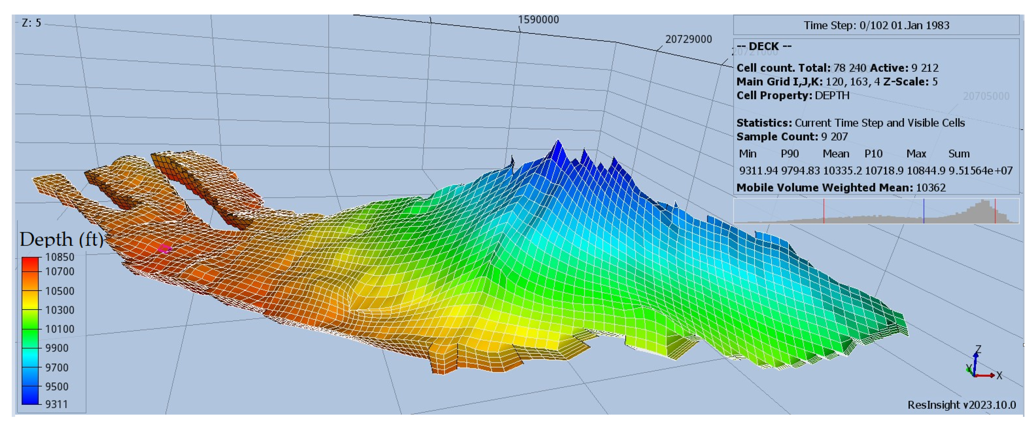
In this study, the sequestration potential of a deep and highly permeable synthetic aquifer (Figure 2) is investigated. The aquifer exhibits an inclined profile, with a pronounced steepness near the crest resembling an anticline, expanding horizontally across a wide area, and comprises four sedimentary layers, each one with varying average permeability values. There is no apparent faulting or fracturing in the formation, and it is assumed to be sealed tightly by shales. The aquifer’s salinity is about 65,000 ppm. Furthermore, it maintains a temperature profile consistent with typical thermal gradient expectations at the reservoir depth. The characteristics of the aquifer can be seen in

Table 1. Aquifer characteristics.

Parameter	Value	Unit
Average pressure (P)	5000	Psi
Temperature (T)	200	° F
Porosity ($\varphi$)	0.25
Average depth (D)	$10,180$	ft
Average xy permeability (k)	300	mD
Bulk volume (V)	$2.4·{10}^{11}$	scf
Water in place	$1.7·{10}^9$	STB

. Due to its high permeability, the pressure distribution within the aquifer adheres to the pressure gradient, remaining isotropic on the x-y plane. The aquifer is considered to be slightly overpressurized, prompting the simultaneous production of brine during CCS operations to postpone reaching the pressure upper safety limit indicated by the technical and safety policies in place as 9000 psi. The significance of this approach is underscored by the zero-flow conditions at the aquifer’s sides, as dictated by no-flow boundary conditions in the simulation model [64].

3.2. BO Framework

To formulate a BO framework, the objective function, its constraints, and the decision variables have to be defined. The target is to maximize the total amount of CO₂ sequestered in the aquifer after continuous injection for 40 years and concurrent brine production with constant target rates. This is handled by introducing two types of groups, injectors and producers, with each group consisting of a number of identical wells.

Constraints are set to the maximum and minimum bottomhole pressure thresholds, as well as to the maximum afforded breakthrough rate of CO₂ recycling. High non-linearity is introduced to the problem by the effect of the wells’ location on the objective function and of the dynamic schedule changes occurring when operational constraints are violated. If, for example, an injector is placed close to a producer, then it is likely that CO₂ breakthrough will occur way sooner than otherwise. Subsequently, the producer will be closed off, and pressure will build up at a faster rate so that the constraint of maximum bottomhole pressure for the injector will be reached sooner, resulting in reduced sequestration. The depth at which each well is situated also plays a huge part in the breakthrough time. Since CO₂ tends to migrate upwards, CO₂ travels faster to a producer situated near the crest. In contrast, if the producer is situated closer to the reservoir bottom, CO₂ breakthrough is delayed. The theoretical maximum amount of CO₂ stored is easily calculated as the target rate of the injectors over the timespan of injection. However, this maximum may be unobtainable due to the constraints already mentioned.

The well placement optimization problem can be formulated as shown in Equation (14).

$$\begin{array}{cccc}\hfill & \underset{\mathbf{x}}{\mathrm{maximize}}\hfill & \hfill & f\left(\mathbf{x}\right)\hfill \\ \hfill & \mathrm{subject}\mathrm{to}\hfill & \hfill & g_i\left(\mathbf{x}\right)\le 0,i=1,2,\dots ,m\hfill \end{array}$$

(14)

where $f\left(\mathbf{x}\right)$ corresponds to the CO₂ mass sequestered, which can be sampled by simulation runs, and $g_i\left(\mathbf{x}\right)\le 0$ are the scheduling constraints, where $\mathbf{x}$ represents the decision variables, which, in this case, are the coordinates $(x,y)$ of each vertical well. Most commercial and research reservoir simulators can embed scheduling constraints into their runs, thus ensuring that the simulation is operationally feasible. This way, the scheduling constraints are handled by the simulator and thus do not need to be explicitly handled by the optimizer. There are, however, additional constraints related to the feasibility of the input space, as discussed in the next subsection. For the optimization process, the python package Bayesian Optimization [65] was utilized.

3.3. Decision Variables and Constraints

Constraints need to be imposed on the input space to define the feasible region of the objective function. For a CCS system with N wells, the input space consists of $2N$ decision variables and the wells’ location may be written as in Equation (15).

$$\mathbf{x}=(x_1,y_1,x_2,y_2,\dots ,x_N,y_N)$$

(15)

The first constraint to be imposed on the input space is that two wells cannot take up the same cells on the grid, since the simulator issues a simulation error instantly. As such, the optimizer is instructed to penalize such cases by giving a very negative value for the objective function when the simulator crashes.

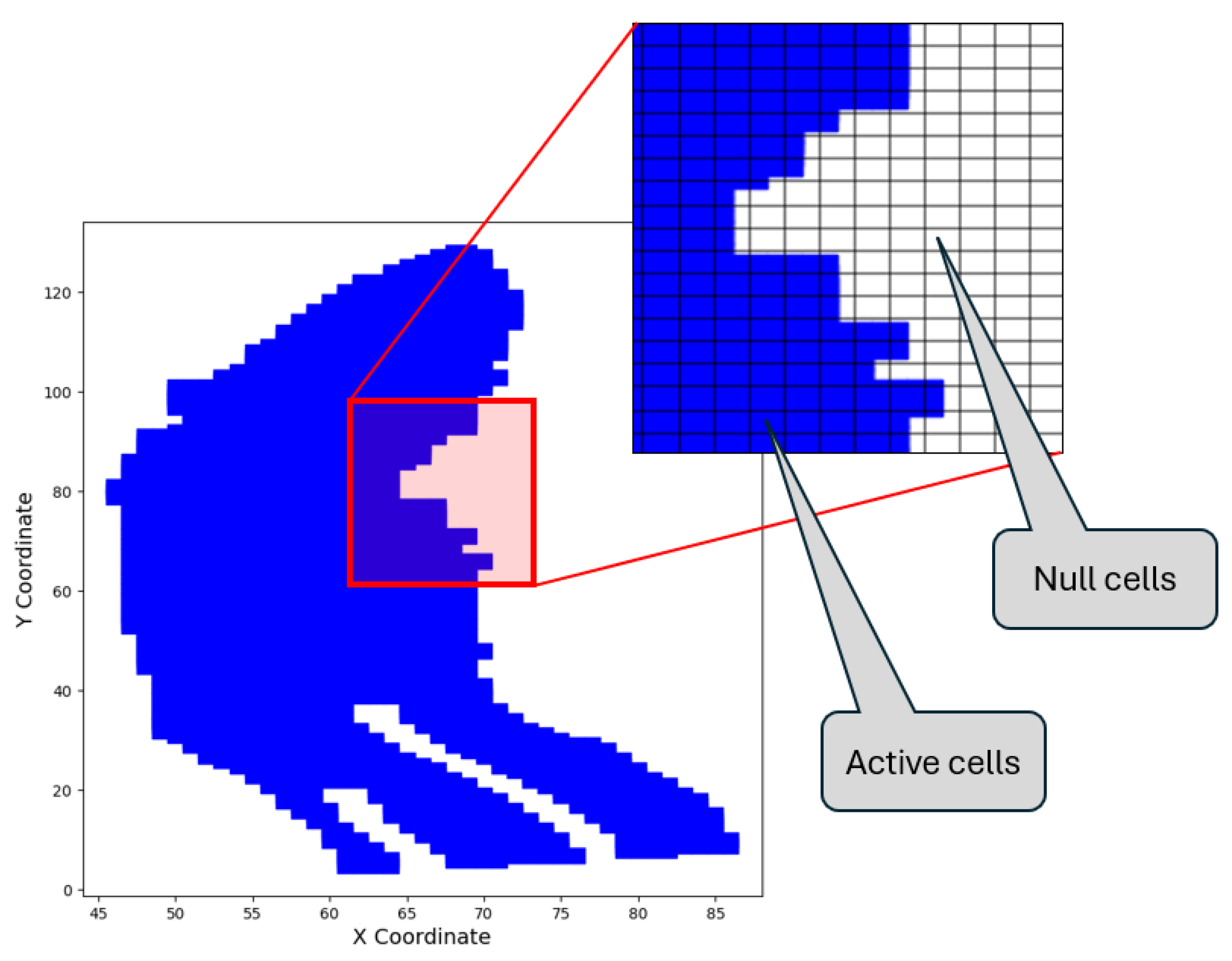
The second and much more troublesome-to-handle constraint is the one regarding the valid position of each well. Since the aquifer’s shape is not a square box, there are coordinate values within the grid-enclosing volume that correspond to null (non-existent) grid cells, as seen in Figure 3. The recommended solution would be to add a severe penalty term by introducing a large negative objective function value for inputs in the infeasible area. For a reservoir with an active-to-total-cell ratio of $50\%$, this ratio corresponds to the probability of a well being placed within the feasible area. If the location of a single well were sought, the optimizer would be able to map the infeasible area quite quickly. However, when N wells have to be placed rather than just one, the probability of selecting all of them inside the feasible space is only ${\left(0.5\right)}^N$. Clearly, the timeframe for the determination of the feasible area increases exponentially with the number of wells selected.

To overcome this challenge, a mapping from this 2D input space to a 1D space is employed while maintaining a one-to-one relationship, using a transformation based on the cell distance from the origin. Subsequently, an ascending-order-sorting operation is applied to the Euclidean norms of each cell to arrange them. Algorithm 1 of the map can be seen below.

Algorithm 1: Mapping function $f:{\mathbb{R}}^2\to \mathbb{R}$.

This mapping is one to one (1-1) because each point $(x,y)\in {\mathbb{R}}^2$ is uniquely associated with a real number $f(x,y)\in \mathbb{R}$. Note that this is not a homeomorphism, as it does not preserve topological properties such as closeness of points.

This mapping allows for dimensionality reduction from a $2N$-dimensional input space to an N-dimensional one. Furthermore, all values in the new input space represent the feasible region, so no more constraints on the input region need to be handled. The mapped values of each cell are shown in Figure 4.

3.4. Permutation Invariance of Input Space

As mentioned earlier, the simulator splits wells into two groups, injectors and producers, managing them collectively under group control policies. Targets and constraints are set for each group, with an embedded optimizer in the simulator responsible for adjusting schedule parameters for individual wells within each group. Essentially, a group comprises wells of the same type, distinguished solely by their location on the grid. On the other hand, the wells’ locations serve as input variables in the BO framework, ordered in a vector. Therefore, the simulator handles the wells’ positions as two sets of unordered objects, partitioned on the respective group, while BO treats them as a vector. Consequently, for the simulator, the input space is invariant under permutations for well positions within a group, whereas for BO, it is not.

Let us consider a scenario following the mapping described in Algorithm 1. If variables m and n represent the positions of injectors and producers, respectively, the input space’s invariance implies that a sampled input exerts the same effect on the simulator, thus also on the objective function, across $m!·n!$ vectors, generated by all of the permutations of the inputs within the same group.

To illustrate this concept, let us consider a simple case with two wells of the same type placed on a $3\times 3$ Cartesian grid (refer to Figure 5). In this scenario, the top-left cell is denoted as [1,1]. Moving right from [1,1] brings us to [1,2], while moving downwards from [1,1] leads to [2,1]. This structure mirrors the conventions of matrix elements, facilitating a straightforward understanding of the grid’s layout. The coordinates for the left sample are $\mathbf{x}=\left(f\right([2,1]),f([3,2]\left)\right)$, and for the right sample, $\mathbf{x}=\left(f\right([3,2]),f([2,1]\left)\right)$, where f is the mapping defined by Algorithm 1. Despite the differing configurations, the simulator produces identical outputs for both samples, since they belong to the same group, and the simulator handles them as a set, regardless of their order. Each sample has its counterpart, or “doppelganger”. As the number of wells increases, the number of potential configurations grows exponentially, since for N wells, each unordered configuration can result from $N!$ different orderings. This example highlights the fundamental principle of group control and the resultant invariance in the input space, offering insights into the system’s behavior regardless of the specific arrangement of wells.

3.5. Modified Kernel Function

The observation of permutation invariance is crucial to better acknowledging the principal idea introduced in this work. Since the black-box function of the BO framework (i.e., the simulator) considers the inputs to be sets, it would be extremely beneficial for this to also be incorporated in the BO framework. By sampling an input vector, information is obtained not only regarding what its objective function value is but also regarding all input vectors that are derived from same-group permutations of its elements. For instance, in the N-dimensional input space, where $N=n+m$, and n and m correspond to the dimensions of the groups, a single sample would give information about $n!·m!$ vectors. It is now obvious that incorporating this information in BO would greatly benefit its efficiency.

To incorporate this in BO, we need to recall that BO builds a surrogate objective function that is mostly influenced by samples and the covariance matrix which is derived from a kernel function. Modifying the kernel function is a clear pathway for improving the efficiency of BO. The kernel function calculates the covariance between points of the input space and acts as a measure of how similar the surrogate objective function’s values are based on the distance between inputs. The Matérn kernel utilized in this work is a stationary kernel, i.e., invariant to translations where the covariance of two input vectors is only dependent on their relative position $k(\mathbf{x},\mathbf{y})=k\left(\right||\mathbf{x}-\mathbf{y}|\left|\right)$. Inputs have high covariance when their distance approaches zero, whereas it decreases as they move further apart.

The modified input space generated by the mapping of Algorithm 1 is useful for generating inputs inside the feasible region, but the caveat is that it is not homogeneous. Points that are close in the modified input space might be very far apart when translated to the original input space. The lack of preservation of this closeness property in the modified input space can be expressed as follows:

$$\mathrm{If}\left|\right|{\mathbf{c}}_1-{\mathbf{c}}_2\left|\right|\le \left|\right|{\mathbf{c}}_1-{\mathbf{c}}_3\left|\right|$$

$$\mathrm{it}\mathrm{does}\mathrm{not}\mathrm{necessarily}\mathrm{imply}\mathrm{that}\left|\right|f\left({\mathbf{c}}_1\right)-f\left({\mathbf{c}}_2\right)\left|\right|\le \left|\right|f\left({\mathbf{c}}_1\right)-f\left({\mathbf{c}}_3\right)\left|\right|.$$

where ${\mathbf{c}}_i$ are cells coordinates and f is the mapping from Algorithm 1. In other words, the mapping function is not an increasing function of the well distance. It follows that if the kernel function utilizes the distances of the mapped input space directly, there will likely be a discrepancy between the calculated covariance and the actual covariance between inputs when this translates to the original input space.

To overcome this problem, the kernel function was modified so that covariance is calculated based on the inverse mapping of the input space, i.e., from the N-dimensional input space to the $2N$-dimensional one which now represents the actual distance between two cells $(\mathbf{x},\mathbf{y})=k\left(\right||f^{-1}\left(\mathbf{x}\right)-f^{-1}\left(\mathbf{y}\right)\left|\right|)$, where $f^{-1}\left(\mathbf{x}\right)=(f^{-1}\left(x_1\right),f^{-1}\left(x_2\right),...f^{-1}\left(x_{11}\right))$. By utilizing this technique, the kernel function now considers the actual distance between two cells.

The last issue to be addressed is the permutation invariance. Since each input vector is invariant under $m!·n!$ permutations, to calculate the representative covariance between two inputs, the permutation ordering that minimizes the distance of the one input to the other needs to be applied. This is a key modification that transforms BO from considering inputs as vectors to now view them as sets. By permuting, it is now able to minimize the distance between sets rather than vectors.

To solve this, a matrix $\mathbf{D}$ is generated, with each value $d_{ij}$ representing the distance of the ith well in $\mathbf{x}$ from the jth well in $\mathbf{y}$, as given by Equation (16).

$$\mathbf{D}=d_{ij}=\left\{\right||f^{-1}\left(x_i\right)-f^{-1}\left(y_j\right)\left|\right|\}$$

(16)

Since the goal is to find the permutation that minimizes the distance between wells in the two samples, the problem can be expressed as finding the permutation of rows (or columns) that minimizes the trace of matrix $\mathbf{D}$, shown in

Table 2. Distance matrix $\mathbf{D}$.

	$y_1$	$y_2$	⋯	$y_n$
$x_1$	$d_{11}$	$d_{12}$	⋯	$d_{1n}$
$x_2$	$d_{21}$	$d_{22}$	⋯	$d_{2n}$
⋮	⋮	⋮	⋱	⋮
$x_n$	$d_{n1}$	$d_{n2}$	⋯	$d_{nn}$

, which has complexity $O(N!)$. Since permutation invariance only affects injectors and producers separately, the problem can be reduced to the two counterparts, i.e., finding the right ordering of the injectors which has complexity $O(m!)$ and finding the right ordering of the producers with complexity $O(n!)$. This is a very well-known problem in the literature called the assignment problem. Algorithm A1 (Appendix A), known as the Hungarian method [66], or Munkres algorithm [67], is commonly utilized to reduce its complexity to the order of $O\left(N^3\right)$, or in our case, $O\left(m^3\right)+O\left(n^3\right)$, saving valuable computational time. Algorithm 2, describing the full Kernel modification, is shown below.

Algorithm 2: Covariance calculation.

    The modified kernel function is represented by a functional form, $k(\mathbf{x},\mathbf{y})=k\left({min}_m\right||$$f^{-1}\left(\mathbf{x}\right)-f^{-1}\left({\mathbf{P}}_m\mathbf{y}\right)\left|\right|)$, where ${\mathbf{P}}_m$ denotes the permutation matrix. This functional form introduces significant non-linearity, due to the involvement of inverse mapping $f^{-1}$ and permutation matrix ${\mathbf{P}}_m$. This non-linearity poses challenges in directly establishing a proof of satisfaction of Mercer’s conditions, which typically rely on simpler, more linear forms of kernel functions. However, despite the inherent complexity introduced by the functional form, extensive sampling efforts across a large number of input samples consistently yield a positive semidefinite covariance matrix. This empirical observation is crucial, as it provides compelling evidence supporting the validity of the modified kernel function. To elaborate, the positive semi-definite covariance matrix implies that the resulting kernel function preserves important properties required for Mercer’s conditions, such as symmetry and non-negativity. The positive semi-definite nature of the covariance matrix indicates that any linear combination of kernel evaluations over the sampled inputs remains non-negative, thus aligning with the requirements of Mercer’s theorem. Furthermore, although direct analytical proof may be challenging due to the non-linearity of the modified kernel, the empirical validation through covariance matrix analysis corroborates the functional form’s adherence to Mercer’s conditions. This empirical evidence, coupled with the observed positive semi-definite covariance matrix, lends strong support to the validity of the modified kernel function despite its inherent non-linearity.

Importantly, due to the permutation invariance inherent in the function, it can be construed as a kernel function operating between sets rather than individual vectors. Algorithm 3 delineates the primary workflow of the Bayesian Optimization (BO) framework employed in this study.

Algorithm 3: Bayesian Optimization framework.

4. Case Study

To properly solve the multi-phase compressible fluid flow problem, reservoir simulation is utilized through OPM’s open-source Flow software v2023.10 [16] (https://opm-project.org/?page_id=19, (accessed on 17 April 2024)). The aquifer is detailed in Section 3.1, while the BO framework is delineated in Section 3.2, Section 3.3, Section 3.4 and Section 3.5. Specifically, $m=3$ injectors and $n=8$ producers are selected. The injector selection is based on the chosen target rates, aligning with commonly utilized practices in CCS projects [68,69]. Conversely, the decision to increase the number of producers is motivated by the requirement for pressure maintenance, particularly in a closed system. This assumption is pragmatic, as it is anticipated that most producers function as lateral extensions of a few multi-segment horizontal wells. A safety upper limit for pressure buildup is set to 9000 psi, while a lower limit of 3000 psi is set to mitigate the need for costly pumping procedures.

4.1. Exploration–Exploitation Trade-Off

The first phase of testing the BO algorithm involves the utilization of all three candidate acquisition functions introduced in Section 2.3, shown in Equations (11)–(13). Each function is utilized twice, once with explorative hyperparameters values and once with exploitative ones. In total, six BO models are generated, with each one being trained through 50 iterations, by an equivalent amount of simulation runs conducted for each model to refine the surrogate objective function. Details of the selected schedule are outlined in

Table 3. Schedule targets and constraints.

Parameter	Value
(Target) Injection rate (CO2)	110 MMscf/day
(Target) Production rate (water)	50 Mstb/day
(Constraint) Max production rate (CO2)	5 MMscf/day
(Constraint) Max bottomhole pressure	9000 psi
(Constraint) Min bottomhole pressure	3000 psi
Duration	$\approx 40$ years
Theoretical maximum sequestration volume (CO2)	$1.58$ Tscf

.

In the table above, “M” denotes 1000, “MM” denotes ${10}^6$, and “T” corresponds to ${10}^{12}$ while “stb” and “scf” represent units of volume, i.e., stock tank barrel and standard cubic feet, respectively, measured under surface conditions. The theoretical maximum volume shown in Table 3 was calculated by multiplying the target injection rate with the duration of the simulation and represents the target value for the optimizer to reach. However, it is crucial to note that this value may not be feasible without violating the imposed constraints; therefore, it may not be achievable under any set of well configurations. Mass-wise, the target injection CO₂ rates correspond to $2.3$ MMtn/yr and the maximum sequestration volume to 90 MMtn.

At first, the performance of all six models is compared in terms of maximum storage value attained by timestep, as seen in Figure 6.

The first component of the series names signifies the hyperparameter value selection guiding the model towards either exploration (XPR) or exploitation (XPT), while the second component indicates the acquisition function employed (see Equations (11)–(13)). It is notable that all models approach a storage result close to the theoretical maximum already by iteration 15. Certain models (XPT EI, XPT PI, and XPR PI) are fortunate to nearly achieve their optimum value early on, possibly due to a lucky initial guess. This suggests that the targeted objectives of the schedule are relatively easy to maintain throughout the simulation. In contrast to other exploitative models, XPT UCB attains an optimal value by the third iteration. Both XPT EI and XPT UCB demonstrate their ability to refine their predictions in later iterations. However, XPT PI peaks at the 10th iteration but fails to reach the $1.5·{10}^9$ mark, likely because PI inherently leans towards exploitation. In contrast, XPR PI continues to exhibit improvements even after 20 iterations. Notably, both XPR UCB and XPR EI consistently find enhancements throughout the iterations, owing to their explorative nature as well as initially exploring sub-optimal regions.

Since the results produced for the max value seem to be heavily reliant on the initial estimation, the distribution of the storage results that each model generated at every iteration is investigated, as illustrated in Figure 7, to offer valuable insights into the impact of the strategy on model performance. Notably, exploratory strategies (illustrated in the right-hand-side plots) demonstrate a higher susceptibility to unfavorable outputs, which arises from their emphasis on exploring uncharted territories within the input space. This trend is clearly evidenced by the elongated tail of the distribution estimation line (kde) and the behavior of the 20th percentile line (dashed green) of the distribution, indicating that these strategies occasionally obtain sub-optimal outcomes. Conversely, exploitative strategies, as indicated by the 80th percentile line (dashed blue), tend to sample inputs that enable them to remain in proximity to the maximum value. However, an exception emerges with XPT PI, which appears to have become stuck in a local optimum, failing to fully capitalize on potential improvements. This divergence underscores the nuanced interplay between exploitation and exploration strategies and their respective impacts on model behavior and performance.

Finally, to give a measure of the well location change per iteration, in Figure 8, the ${\mathcal{L}}_1$ norm between the locations in subsequent iterations is depicted as “Vector Distances” defined as the trace of matrix $\mathbf{D}$, as shown in Table 2, aiming to offer insights into the level of exploration across the models. However, since distance alone is not the optimal metric due to permutation invariance, akin to the modification of the kernel function, the “Set Distances” value between subsequent runs is calculated, utilizing Algorithm A1 on $\mathbf{D}$ to yield the minimum distance. This approach offers a more accurate depiction of the exploration dynamics among the models, mitigating the limitations associated with the traditional distance metric.

The median of the “Vector Distances” series of exploration strategies is clearly higher than that of exploitation ones, as exploration inherently involves probing a wider range of input space. However, it is noteworthy that due to the acquisition function not being directly dependent on the kernel, the Set Distances value between the inputs is considerably higher in exploitative strategies. This observation suggests that exploitative strategies ultimately explore the space more efficiently. In essence, while exploration strategies cover more ground in terms of distance, exploitative strategies manage to navigate the space effectively, potentially due to their focused search around promising areas guided by the acquisition function.

4.2. Kernel Comparisons

To further evaluate the performance of the proposed method, a comparison between the modified kernel against the original Matérn kernel and an approach that randomly selects well positions is presented. This test is performed on a more strenuous schedule having a higher target injection rate, increased by more than 50%, as seen in

Table 4. Schedule targets and constraints.

Parameter	Value
(Target) Injection rate (CO2)	170 MMscf/day
(Target) Production rate (water)	77 Mstb/day
(Constraint) Max production rate (CO2)	5 MMscf/day
(Constraint) Max bottomhole pressure	9000 psi
(Constraint) Min bottomhole pressure	3000 psi
Duration	≈40 years
Theoretical maximum sequestration volume (CO2)	$2.44$ Tscf

. The target injection rate now corresponds to $3.6$ MMtn/yr and the maximum sequestration volume to 142 MMtn.

This comparison aims to elucidate the impact of the two modifications made to the kernel described in Section 3 on the final outcome. Specifically, we seek to understand their influence on the end result, as well as their ability to expedite the optimization process. The acquisition function utilized is EI with moderate hyperparameter values, striking a balance between exploration and exploitation. By evaluating these aspects, valuable insights can be gained into the efficacy and efficiency of the proposed modified kernel in comparison with both the original kernel and a random selection strategy.

As illustrated in Figure 9, the modified kernel surpasses the two alternatives in terms of maximum CO₂ sequestered. Furthermore, it demonstrates consistent improvement, initiating enhancement as early as at the third timestep and continuing to refine its performance a total of four times before the 15th timestep. In contrast, the original kernel demonstrates improvement only twice, and its performance is comparable only to that of the random process. This stark discrepancy underscores the critical importance of effectively managing kernel functions. Failure to comprehend and address the nuances of optimization caveats would have hindered our ability to achieve such promising outcomes.

Notably, the original kernel function’s performance is akin to that of a random process. This outcome is attributable not only to improper distance calculations based on the 1D modified input space in the covariance but also to the lack of comprehensive information regarding permutation invariance and the need to manage a considerably larger input space as a consequence. Figure 10 further supports this argument by demonstrating that the density distribution of the results of the original kernel and the random optimization are very close, as opposed to the modified kernel’s results, where the density function is clearly skewed towards the optimal value.

5. Discussion

To facilitate a broad discussion on the modifications and the results presented so far, a brief synopsis of what has transpired thus far needs to be presented. The objective of this work is to apply a BO framework to optimize well placement in a CCS project. Rather than applying BO in a “out of the shelf” straightforward fashion, several key modifications and analyses outlined throughout Section 3 were employed, aiming at enhancing optimization efficiency and effectiveness. Firstly, by utilizing a formation with complex geometry rather than a simple “sugar box”, the issue of infeasible areas within the input space emerged and had to be addressed by implementing a transformation technique. This step allowed us to circumvent infeasible regions that took up the majority of the original input space.

This modification was not tax-free, as it introduced a severe issue to the kernel. The non-homeomorphic nature of the map implied that kernel closeness of points in the new modified input space did not translate to the same closeness on the original, thus violating the need for the kernel function to calculate the covariance properly. To address this, modifications were further introduced to the Matérn kernel, utilizing inverse mapping to capture real distances between well positions. By recalculating covariances based on actual distances, this adapted kernel accurately represented the spatial relationships crucial for optimal well placement.

A significant advancement in the proposed methodology was the integration of our knowledge of permutation invariance into the kernel function. From a mathematical point of view, this innovation enabled the kernel to operate on sets rather than conventional vectors, effectively considering the minimum distances between well positions under permutations. The resulting kernel showed to be instrumental in improving optimization outcomes, as demonstrated through rigorous experimentation in Section 4.2, where BO was run with and without the proposed modifications, with the results being significantly better in the modified case.

Clearly, the modified kernel exhibited superior performance, highlighting its pivotal role in driving significant improvements in well placement optimization outcomes. It is our strong belief that a solid foundation has been laid for future research endeavors aimed at optimizing the well placement problem with enhanced precision and efficiency. The proposed method is generalizable to other applications of well placement optimization, not necessarily restricted to a BO framework as long as wells operate under group control, making the input space invariant under permutations. These modifications can also find applications in other learning algorithms characterized by permutation invariant inputs.

In addition to the comparisons presented thus far, it is important to address the optimal placement identified by the algorithms and consider what insights engineers’ intuition could offer. Generally, in a closed system, producers and injectors should be positioned as far apart as possible. For this aquifer, an alternative configuration could involve injecting CO₂ at the crest and placing the producers around the periphery, which would potentially enforce the resulting plume to remain relatively stationary and not descend as rapidly. 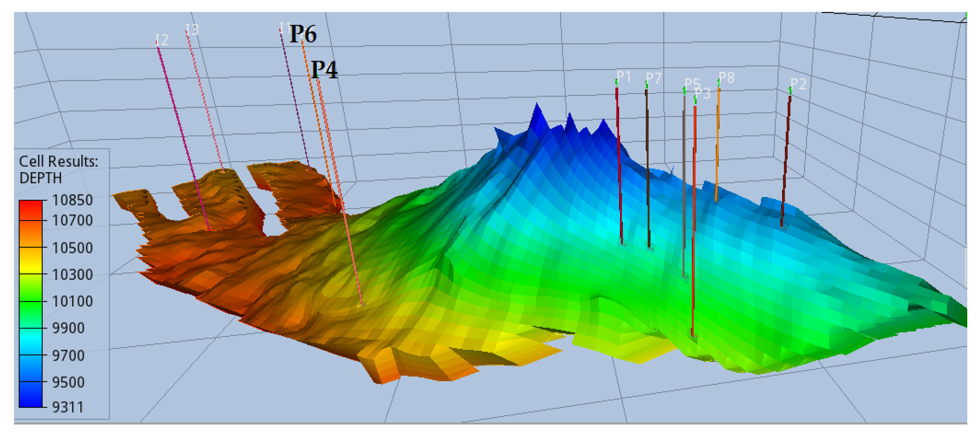As depicted in Figure 11, the solution derived by the BO algorithm reflects a blend of both engineering perspectives and considerations.

Injectors are strategically positioned as far away as possible from the majority of the producers, situated in the region resembling a fork at the base of the aquifer. Conversely, most producers are sited on the opposing side of the crest that resembles a “hill”. CO₂ naturally migrates upwards, facilitated by a clear pathway to the crest. It is reasonable to assume that producer P6 is strategically placed along the anticipated path of the plume for pressure maintenance, given the substantial injection rate from day 1. Producer P4 is strategically located to ensure a uniformly distributed plume. Considering the gravitational pressure differential that causes CO₂ to migrate towards the crest, the advancement of the resulting plume’s front would be uneven. However, P4 counteracts this by moderating the pressure in its vicinity, resulting in even plume migration by the end of the CCS period, as illustrated in Figure 12.

Finally, the remaining six producers are positioned behind the crest, in accordance with the second intuition, that is, the deceleration of the CO₂ plume once it reaches the crest, primarily due to density differences between CO₂ and the brine. At this juncture, breakthrough to the producers becomes inevitable, marking the conclusion of the injection period. It is noteworthy that the simulation ran successfully for approximately 40 years, during which the injection rate naturally decelerated due to pressure buildup. However, as depicted in Figure 13, the plume had not yet reached the producers by this point.

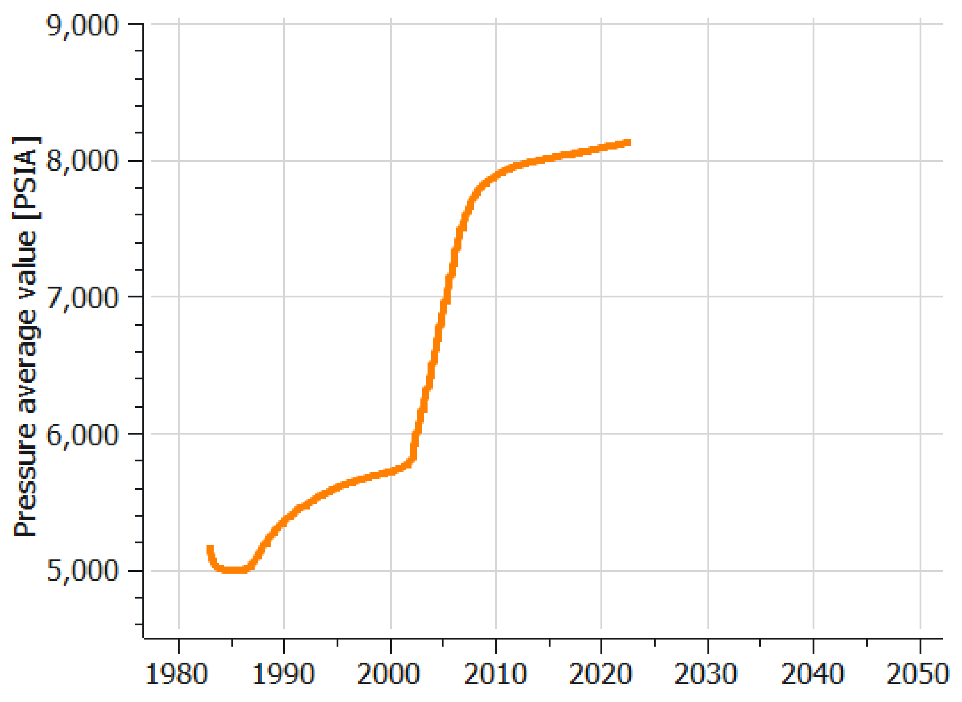
   Field pressure, depicted in Figure 14, is shown to emphasize that even after 40 years of continuous development, the aquifer has not yet reached the safety limit pressure. Pressure gradient varies due to the constraints imposed on production/injection and breakthrough rates.

   Overall, BO optimization successfully captured, without any explicit guidance and in a very limited number of simulation runs, the need for producers and injectors to be spaced as further apart as possible, while positioning the producers below the crest to slow down CO₂ plume breakthrough. These are the two primary insights crucial for injection optimization, which an experienced engineer would typically independently deduce. Configurations deviating from these principles are deemed sub-optimal, leading to earlier CO₂ breakthrough in producers. Consequently, producers are prematurely closed off, pressure builds up faster, and injection rates decline sooner, resulting in reduced total CO₂ injection and less effective plume sweep efficiency. This trend is illustrated in Figure 15, where the optimal case’s injection rate (blue line) is compared to a sub-optimal one (red line). Despite the optimal case having a notably higher target injection rate, it maintains this rate for over a decade longer and exhibits a more gradual decline compared with the sub-optimal scenario. In the latter, injectors are not efficiently spaced with respect to the producers; therefore, the pressure reaches the safety limit of 9000 psi in less than a decade of development. The number of producers and injectors, as well as the aquifer system, are identical in both cases.

Given the engineering-oriented approach of the optimizer’s solution, there is a high degree of confidence that the proposed solution is indeed optimal. However, it is essential to acknowledge the complexity introduced by the multi-dimensional nature of the input space. While the solution obtained represents a significant achievement, it is plausible that there exist alternative configurations capable of matching or even surpassing this optimal value. Furthermore, an interesting consideration arises from the spatial proximity of the six producers. Given their close positioning, there is potential for aggregation into one or two total producers during the project’s design phase. Consolidating these producers could streamline operational logistics and potentially optimize resource utilization, contributing to further efficiency gains. After performing multiple simulations, aggregating the six wells into one or two and considering the rates of the optimized case, it was seen that the total volume of sequestered CO₂ slightly dropped by 3–7%, which could of course be negated by the reduced costs of drilling so many wells. However, a complete evaluation of this trade-off is beyond the scope of this work.

6. Conclusions

In this study, the well placement optimization problem was handled as a Bayesian Optimization one. To our knowledge, this was the first attempt of applying BO in a well placement CCS setting. The analysis focused on several key modifications and comparisons to enhance the efficiency and effectiveness of the optimization process. Firstly, the issue of the input space’s infeasible area was addressed by introducing a mapping to a modified input space. This adjustment allowed the algorithm not to be concerned with exploring the infeasible regions by itself, a process which would require hundreds of thousands of iterations. Furthermore, a novel kernel modification was proposed, aiming at achieving invariance under permutations of the input vectors. This adaptation not only enhanced the robustness of the optimization process but also ensured that the model’s performance remained consistent across different permutations, a crucial consideration in real-world well optimization.

Subsequently, comprehensive analyses were conducted by using various acquisition functions, including expected improvement (EI), upper confidence bound (UCB), and probability of improvement (POI). Through comparative graphs, the performance differences among these functions was illustrated, providing valuable insights into their respective strengths and limitations in the context of CCS well placement optimization. One of the primary contributions of this study was the comparative evaluation of the developed modified kernel against its unmodified counterpart and a random function. The obtained findings unequivocally demonstrated the substantial impact of the modified kernel on optimization efficacy.

After extensive testing, we successfully optimized the sequestration of CO₂ in a saline aquifer. The resulting scenario reflects both intuitive engineering principles and computational efficiency. Our efforts culminated in a comprehensive case study outlining the optimal sequestration of 115 million tons of CO₂ over a four-decade period. This achievement represents 80% of the theoretically maximum value of 142 million tons, signifying exceptional efficiency within a closed system. Typically, breakthrough and pressure buildup pose significant challenges in such processes, often limiting their duration and effectiveness.

In conclusion, this study significantly enriches the ongoing discourse surrounding Bayesian Optimization and its practical implementation in complex domains like CCS. Through the introduction of bespoke modifications and comprehensive comparative analyses, a solid foundation for future progress in optimization methodologies has been established, tailored specifically to the nuanced challenges of real-world scenarios. Our efforts pave the way for further refinement and expansion of these techniques, bringing us ever closer to harnessing the complete capabilities of Bayesian Optimization in addressing the intricate well placement problem. Moving forward, the exploration of advanced exotic Bayesian Optimization procedures and frameworks becomes a priority, thereby pushing the boundaries of optimization capabilities in CCS and related fields. This includes extending our methodology to accommodate various types of wells, such as horizontal, inclined, and multi-segment wells, which pose unique challenges due to their non-traditional geometries and flow characteristics. Additionally, the importance of addressing geological uncertainty and the complexities of diverse formations is recognized; thus, future research endeavors will focus on incorporating these factors into the optimization framework. Furthermore, to enhance the industry relevance and real-life applicability of this research, the integration of a net present value (NPV) objective function into the optimization model is intended to be incorporated. This addition will enable the direct optimization of well placement decisions based on economic considerations, aligning our approach more closely with the priorities and objectives of stakeholders in the CCS industry. By integrating NPV considerations, we can ensure that our optimization solutions not only meet technical requirements but also deliver optimal economic outcomes, thereby facilitating more informed decision making in real-world CCS projects.