1. Introduction
Technologies that efficiently harness the power of ocean waves are now emerging, setting the stage for ocean waves to become a new major renewable energy source [
1,
2]. These technologies have great potential and can be used in tandem, with other renewable energy sources, such as wind and solar, to cater to peak energy demands. Various groups have successfully developed several types of wave energy converters (WECs) at the lab scale, and several models have now been installed in the oceans for commercial testing [
3,
4].
In order to permit analytic development, the optimization procedure and control strategy should be considered. The optimization is to determine the parameters of the model geometry and the physical component under constraints [
5,
6,
7,
8,
9]. In addition, the control strategy for how to tune the power take-off (PTO) needs to be determined to maximize the consistency of the extracted power in response to the wave variation in height and frequency due to changes in the ocean environment condition from hourly to annually. Initial studies employing the control strategy for WECs revealed that impedance matching provides the theoretical maximum useful energy for a body oscillating in one mode [
10,
11,
12]. However, this strategy requires a preemptive knowledge of the body’s velocity and/or excitation force of the waves, making it impossible to implement in practice. Furthermore, it requires an ideal (or close to ideal) PTO, which must be able to readily switch between the functional roles of a generator and actuator with high converting efficiency. This in turn would allow control over the sign and magnitude of the hydrodynamic stiffness and the damping coefficient [
13,
14].
One of the control techniques that requires a relatively low level of WEC’s hydrodynamic information with a reactive energy flow is latching control. This method was first applied to a single heaving buoy [
15] and was later also applied to two-body systems [
16,
17]. This technique only requires the stopper and not the actuator function of the PTO. However, it does require information regarding peak moments of upcoming ocean waves.
Oscillating water column (OWC)-WECs have also been widely studied. OWC-WEC, which is simpler in terms of configuration, was first designed for use in marine navigation [
18,
19,
20]. Later, OWC-WEC research mainly focused on fixed systems along the coast [
21,
22,
23] and floating systems on the open sea [
7,
8,
24,
25,
26].
OWC-WECs essentially consist of a capture chamber, a turbine and an electrical generator. Compared to the moving body types, they have a relatively simple mechanical structure, since there is no mechanical elements, such as a hinge, shaft or linear guide. Incident waves cause the inner water surface level of the capture chamber to oscillate. The reciprocating air flow resulting from the pressure fluctuations in the chamber drives the turbine. The electric generator connected to a turbine rotor then converts the rotational kinetic energy into electricity. The direction and speed of the air flow supplied to the turbine are frequently changed via movement of the waves. As such, an impulse turbine [
27,
28] or Wells turbine [
29], which rotates in one direction regardless of the direction of air flow, is commonly fitted to circumvent the air to the electricity energy conversion problem in OWC-WEC systems.
Efforts have been made to improve the efficiency of OWC-WECs by using a control strategy. However, as an impedance matching control, the PTO module itself acts as an ideal actuator. In OWC-WEC, the self-rectifying air turbine, which functions as the PTO module is unable to work as an actuator. As a result, in order for the impedance matching control to be applied to OWC-WEC, a highly-efficient compressor must be introduced to make its application impractical [
30,
31,
32]. Jefferys et al. [
33] presented a latching control strategy for OWC-WEC, which considers air compressibility. Hoskin et al. [
34] were the first to apply a phase controller to the OWC-WEC by making the damping coefficient proportional to the device’s velocity. These studies all aimed at developing strategies to maximize the conversion efficiencies in the chamber stage (first stage). However, since OWC’s overall efficiency is also influenced by the turbine stage (second stage), control strategies to ensure the turbine’s efficiency would also be of benefit to the system. The power of air flow induced by the water column oscillation is transferred to the turbine, and the resultant turbine rotation in turn affects the motion of the water column. Thus, control strategies that consider the entire system including the turbine stage were introduced in [
6,
35,
36,
37,
38,
39].
In [
6,
35,
36], the frequency domain analysis is introduced to calculate a large number of simulations that consider various ocean states. It is assumed, however, that the turbine rotational speed remains constant, thereby resulting in a large rotational inertia. However, under these conditions, the turbine cannot respond in a low level of sea energy state. In addition, since this analysis is done in the frequency domain, the moment controller strategies in the time domain were not allowed.
In [
37,
38,
39], control strategies to avoid stalling were introduced, since when using the Wells turbine, stalling drastically reduces the efficiency. These analyses were based on the Newtonian mechanics, so performed in the time domain, and analyzing the effect of the control strategy impact on the turbine stage was carried out. Because the effect of turbine stage on the chamber stage is not taken into account, the effect of control strategy impact on the overall system efficiency was not analyzed.
In summary on the previous studies on the optimization and control theory of OWC-WECs including turbine aerodynamics, it can be mainly categorized as the frequency domain analysis and time domain analysis; they have their own pros and cons. The analysis of the frequency domain takes into account the compressibility of air and provides the direct substitution of the wave spectrum into the analysis, but the turbine aerodynamics based on the Newtonian mechanics is impossible, which brings the assumption of the turbine’s constant angular speed [
6,
35,
36]. Otherwise, the time domain analysis is able to address the angular acceleration of the turbine rotor since it is based on the Newtonian mechanics [
27,
28,
37,
38,
39]. Therefore, it is not necessary to assume the constant angular speed of the turbine rotor.
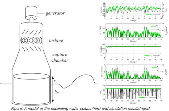
We choose the time domain analysis in order to develop a real-time control law for OWEC-WECs considering turbine aerodynamics. We investigate a system that combines the hydrodynamics of the chamber, the aerodynamics of the impulse turbine and the modeling of an ideal DC generator, as shown in
Figure 1. Unlike the analysis in the frequency domain, analysis in the time domain is based on the Newtonian mechanics, and it considers the angular acceleration of the turbine rotor. In the turbine aerodynamics, the pressure on the turbine, induced torque from the electric generator and turbine rotor inertia are taken into account and determine the angular acceleration of the turbine rotor in real time. Accordingly, it requires no assumption of constant rotor angular speed for the frequency domain, and rotor inertia acts as an important variable.
We put forth two strategies for the controller. First is a strategy that maximizes the turbine’s instant efficiency. The second strategy attempts to maintain the rotational speed at a constant rate. These two methods are differentiated by the definition of the reference angular velocity and can be induced by the Lyapunov stability theory [
40,
41,
42,
43]. The aforementioned controllers can be implemented by a load control that is attached to the ideal DC generator. We investigate the performance of the controllers through simulation in the time domain under irregular waves. Furthermore, we run simulations in various wave periods and heights and compare and analyze the performance of the strategies with and without the controller.
3. Controller Design and Stability Analysis
3.1. Control Design Objective
A majority of research on control strategies for WECs has focused on the first stage of the system [
17,
34,
47]. Here, we will only focus on that of the turbine stage. Previous studies have dealt with control strategies of an OWC-WEC with the turbine module [
9,
35,
36]. These papers assume that blade inertia is large enough for the turbine angular speed to remain constant. However, these studies do not cover the effects of electric generator load on the turbine system in the time domain.
In the previous section, our turbine modeling provides the input states ( and ) and the outputs (Ω and (or )). Here, we emphasize that is the only controllable parameter. Thus, this study presents control strategies for the impulse turbine where the control input is .
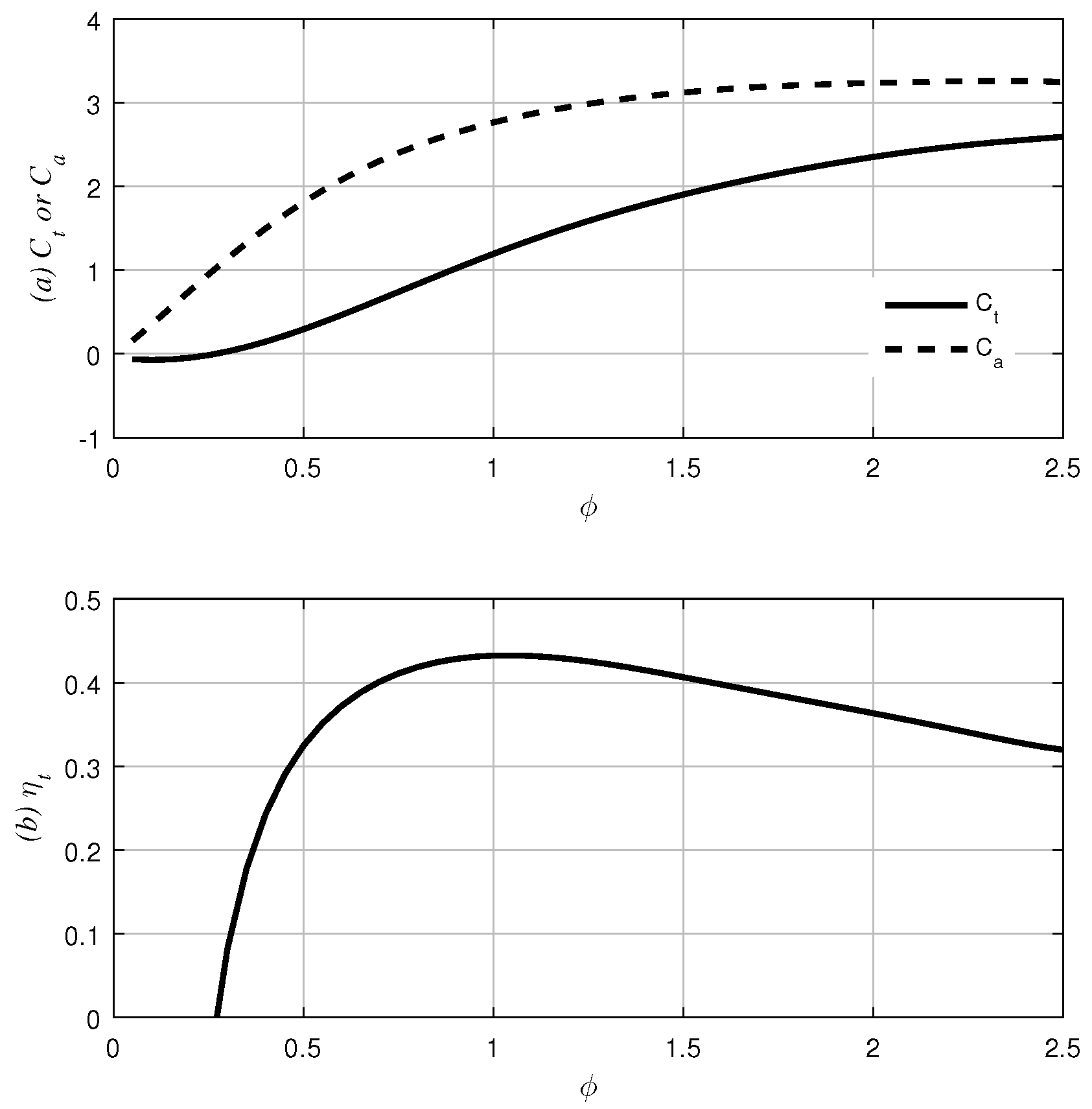
Two major issues arise when considering the turbine’s characteristics and power quality. These issues relate to (1) the maximum turbine efficiency and (2) the constancy of the output voltage. As shown in
Figure 2, the efficiency of the turbine is a function of
ϕ and has a single peak point. This optimal point will herein be referred to as
. For the first issue, it can be determined from (
7) that the reference rotor angular velocity (or desired angular velocity)
becomes a function of time varying state
as:
Consequently, the control objective for the maximum turbine efficiency is to make Ω track the time-varying desired angular velocity .
Furthermore, a constant supply of voltage is important for the quality of generated electric power. It is hugely advantageous to provide a constant voltage in terms of usability and workability while providing irregular current. Whether charging a battery directly or connecting it to the converter, electricity with a constant voltage is more utilizable than that with a constant current. Equation (
14) states that the output voltage is proportional to the rotor speed. As such, generating a constant output voltage relies heavily on maintaining a constant rotor speed. Thus, for the second issue, the control objective is to make Ω converge to the constant desired angular velocity
.
It should be noted, however, that maximum turbine efficiency and constant output voltage cannot be simultaneously achieved. Hence, upon reaching maximum turbine efficiency, the output voltage must be swung according to . Conversely, if a constant voltage output is achieved, the turbine efficiency will subsequently be sub-optimal. Nonetheless, both parameters are determined by Ω, and consequently, choosing will determine the control purpose. From this point, the former will be referred to as the i-MET (instantaneous-maximum efficiency tracking) control and the latter as the CAV (constant angular velocity) control, respectively.
3.2. Stability Analysis
We present the i-MET and CAV controllers using stability analysis based on Lyapunov’s theory [
40,
41,
42,
43]. We use the damping coefficient of the generator
as a control input. This value must be positive since it is assumed that the electric generator can only convert kinetic energy to electric energy, while the reverse process is not possible. Thus, our analysis assumes that this controller only performs with a positive
value. As mentioned above, both controllers share the objective of tracking
. However,
for the i-MET strategy is time varying, whilst
for the CAV strategy remains constant.
Consider the dynamic equation of the system obtained from (
12) and (
13) as:
With tracking error
, the control law can be designed as:
where
,
and
is a switching variable with
and
.
In order to derive the control law, let us define the Lyapunov candidate as:
The time derivative of (
21) with substituting (
20) yields:
Using the following the hyperbolic tangent function property (
ζ: real number):
yields:
where
.
Multiplying (
24) by
and integrating over
provides:
Therefore, disappears in as time increases and converges with a boundary of . c is the settable variable and defined as an arbitrarily small constant. As a result, the tracking error becomes arbitrarily small. In the process of the stability proof for the controller, Ω becomes with small margin of error.
4. Simulation Results under Irregular Waves in the Time Domain
We carry out simulations of the OWC system associated with the control strategies in the time domain. For time domain calculations, a Runge–Kutta method [
48] was applied for solving the above dynamics under irregular wave condition.
We obtain the hydrodynamic parameters of the first stage from ANSYS AQWA [
49] using the assumption that a trapped water column is regarded as a rigid body of a cylindrical shape. In the simulation, the body has a 6-m diameter with a 5-m draft (
) floating in the ocean cube that has a 500 by 500
surface and a 50-m water depth, and only the heave motion of the body is allowed. In order to properly calculate heave impulse response function, the frequency domain response should have a truncation frequency of 2 rad/s with a frequency spacing of 0.05 rad/s [
50].
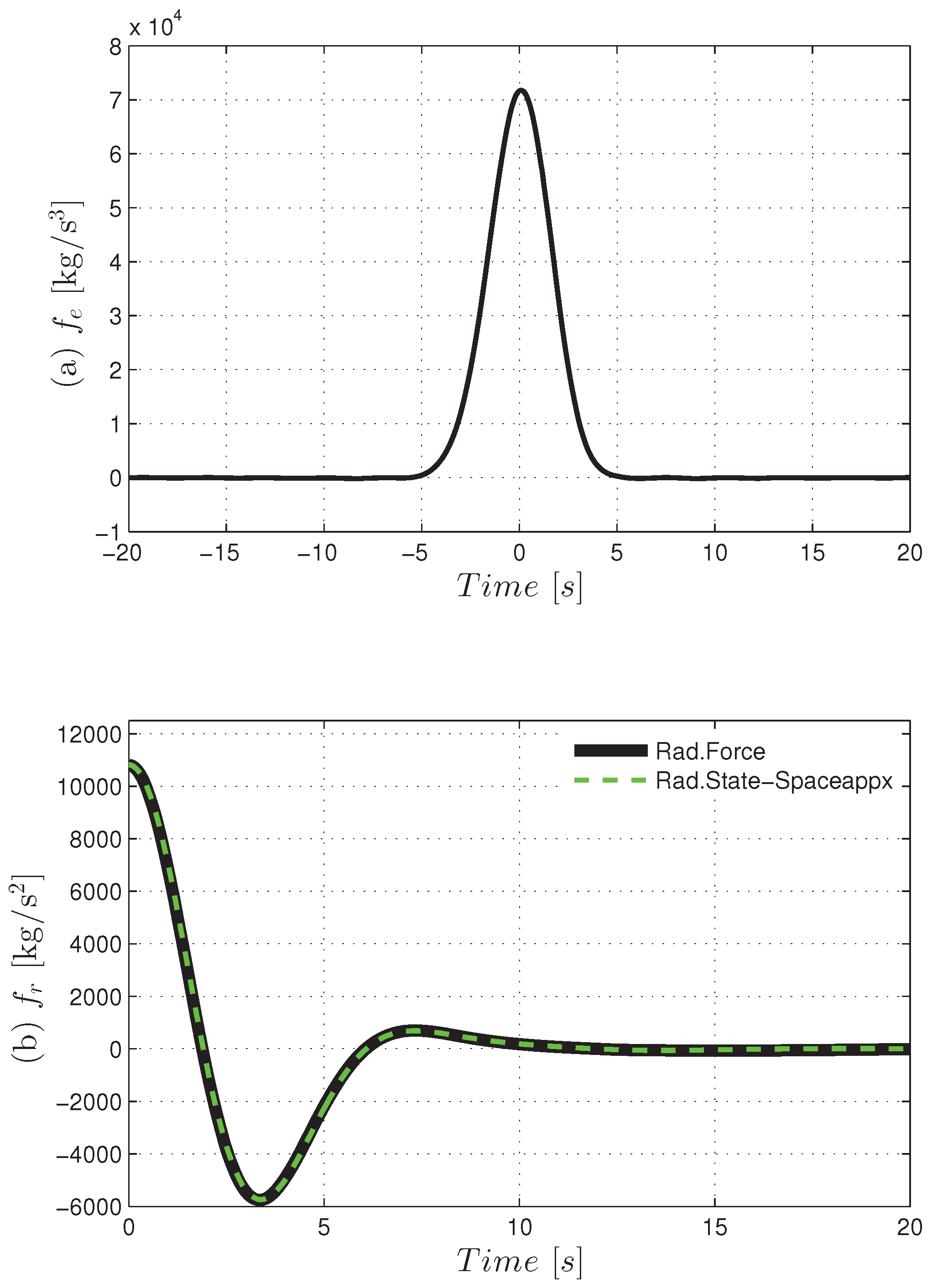
The solid lines in
Figure 3 display the impulse response of excitation force
and radiation force
for calculations of
and
, respectively, and the dashed line is for the state space approximation for
.
A Pierson–Moskowitz (PM) wave model is applied to analyze the performance of the device. When a constant wind has blown for a sufficiently long time along a sufficiently long stretch of the ocean, the semi-empirical PM spectrum [
51]:
matches relatively well with the experimentally-obtained wave spectra, where
and
denote significant wave height and the peak wave period, respectively.
For time series calculations, the spectral distribution (
26) is discretized as the sum of a large number
N of regular waves as written as:
Here,
, where
is the lowest frequency,
is a small frequency interval,
and the spectrum is not to contain a significant amount of energy outside the frequency range
.
and
are the amplitude of the wave component of order
n and the initial phase randomly chosen in the interval
, respectively. A summary of the parameters and values used in calculations is given in
Table 1.
We performed the simulation under various wave heights and periods, but only one condition was chosen for verification of the controller operation under irregular waves with and . The sampling time interval is 0.02 .
4.1. Result of the i-MET Controller
We carry out the simulation of an OWC-turbine combined system with an i-MET controller given as (
20) with (
18) under the PM wave condition in the time domain using a fourth order Runge–Kutta method. Between all i-MET controller’s gains
,
γ and
ϵ,
had the greatest effect on the controlled result. Therefore, with fixed gains
γ and
ϵ set at 100 and 0.01, respectively, we observe the difference in performance with varying
values.
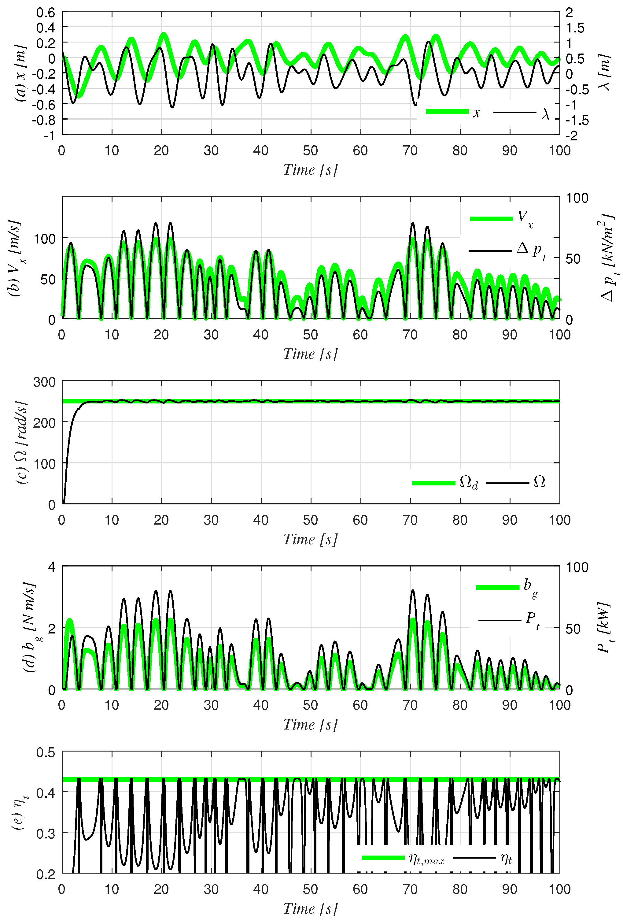
Figure 4 and
Figure 5 show the results of the first 30 s of the simulation, when
is set at 0.5 and 10, respectively. It can be observed in both graphs that
changes consistently to follow
by (
18) with the fluctuation of
. Through comparisons between both graphs, however, it can be seen that a result of
produces a better performance than that of
in terms of control purposes, since Ω tracks
closer and more quickly. This yields that the longer duration of the instant efficiency
is able to reach the maximum value with
.
To improve the accuracy of our analysis, we obtained values for average power extraction from the turbine
, average turbine efficiency
and the relative root mean squared error of Ω (
) by changing
to a value between 0.1 and 10 for 5000-s intervals (
).
is expressed as the ratio between the time integral value of the pneumatic power and the power extraction from the turbine.
is the relative root mean squared error of the Ω with respect to average desired angular velocity
for the times when the controller is functioning. These can be expressed as follows:
Here, and represent the beginning and the end times, respectively, of when the controller is working at the n-th order, which is equivalent to .
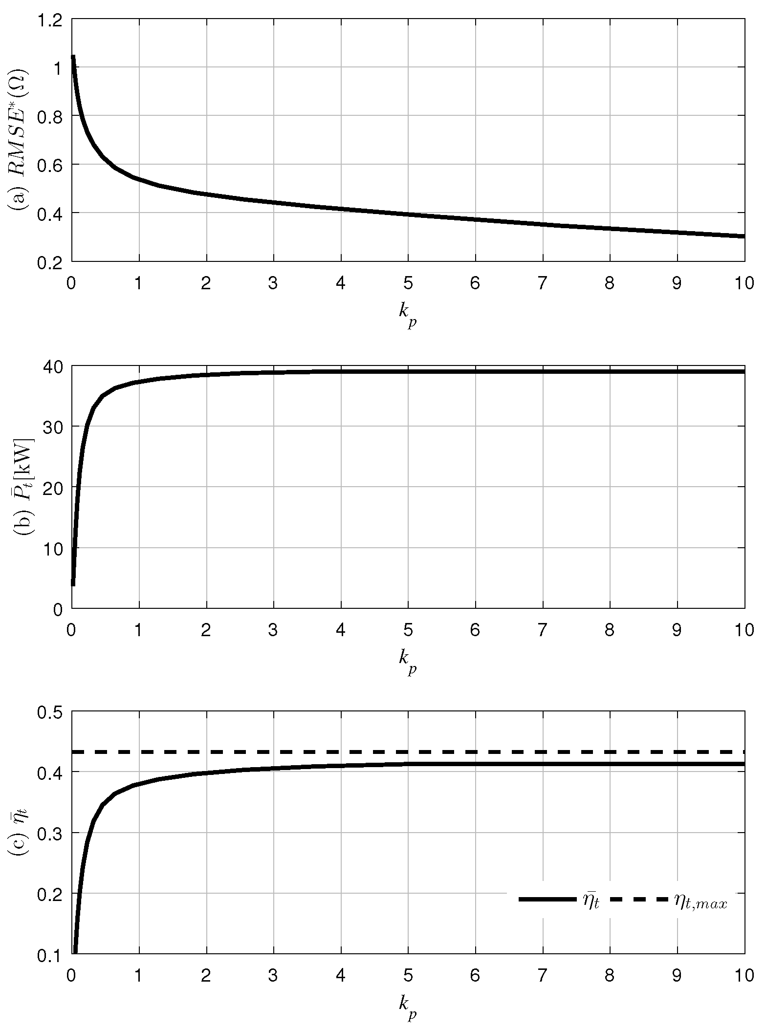
Figure 6 reveals that
and
increase as
increases. Beyond a
value of five,
and
reach a plateau, and no improvement of them can be observed. Conversely, as
increases,
decreases drastically. Therefore, it appears that the optimal performance of the i-MET controller is reached as
increases. However, as seen in the
Figure 5, when
,
tends to generate abnormal peaks as
converges zero.
4.2. Result of the CAV Controller
In order to evaluate the performance of the CAV controller, we set the as a constant to run the same simulation previously performed under the equivalent irregular waves, having a PM spectrum with and .
There are three factors that affect the CAV controller’s performance:
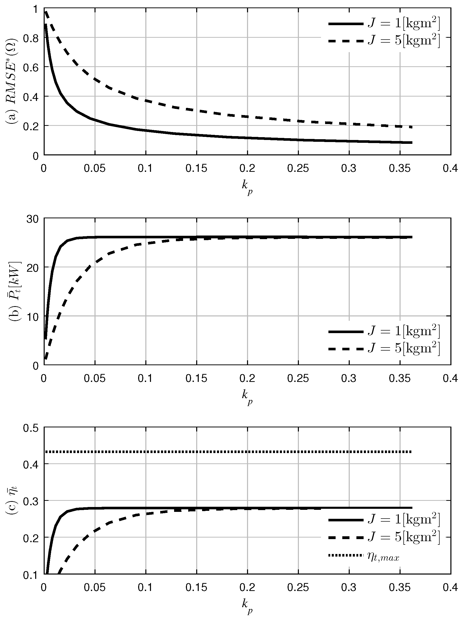
,
and the inertia of the turbine and generator rotors
J. Note that when
is constant, the variation of Ω decreases as
J increases. We first sought to observe the influence of
in the time domain.
Figure 7 and
Figure 8 depict the simulation results of the OWC-turbine combined system with the CAV controller in the time domain where
0.05 and 1, respectively, and
. Through comparing the two figures, it is apparent that a
value of one provides a faster convergence speed with a smaller error bound of Ω.
When
is at one, Ω converges to the
. However, in both cases, we observe that the time interval of the maximum value of
is drastically reduced compared to that of the i-MET controller, as seen in
Figure 5. Furthermore, as seen in
Figure 7 and
Figure 8, the peaks of
and
are unmatched, causing the turbine’s performance to have a negative effect on the total output.
In order to more accurately observe the power extraction and the convergence of the angular velocity, we measured and compared their average values over a period of 5000 s.
Figure 9,
Figure 10 and
Figure 11 show the
, average turbine power extraction
and the average turbine efficiency
, with respect to
, when
is at 250, 400 and 550 rad/s.
As seen in
Figure 9,
Figure 10 and
Figure 11,
converges to zero as
increases, as intended for control purposes. It should, however, be emphasized that the curve of
with
is lower than that with
regardless of
in all cases. The CAV controller functions better when the inertia is smaller. This runs contrary to the results given when not using a controller. Hence, when not using a controller, a larger inertia results in smaller angular speed variation.
Unlike , which is the inverse of independent of , the average power extraction and average turbine efficiency behave differently depending on the reference angular velocity .
The optimal average power extraction and average turbine efficiency is achieved when
(
Figure 10). It should be noted that under these condition, when
increases,
, and
also increase. However, when
, the increase in
does not result in an overall increase in
and
(
Figure 11).
To summarize, the convergence of the angular velocity is predominantly affected by the control gain , while the average power extraction is influenced mainly by the reference angular velocity .
5. Simulation Results under Irregular Conditionsfor Various Wave Period and Height
Here, we analyze differences between two previously-mentioned types of controllers in the set time domain. We show that increasing the instant efficiency of the turbine or maintaining a certain angular velocity will effect the converting efficiency of the chamber stage. Therefore, an analysis of how the overall system, including the chamber stage, influences the overall power output is needed.
In brief, our system consists of a chamber, turbine, DC electrical generator and terminal load attached to the generator. Due to the assumption that the only controllable parameter is the damping coefficient
, which is produced by the generator and decided by the load, from the electrical analysis point of view, the analysis with the simplest electrical component should precede, and constant linear damping is produced from the simplest electric component, the resistor. Additionally, the constant resistor
in (
16) provides the constant damping coefficient
. Accordingly, we choose the results of constant damping
as the comparison results group for the controlled results. We set the standard as the maximum power extraction when
is at a constant.
Similar to the previous simulation, we measure the average power extraction
with the same chamber, turbine and ocean state, when
is held constant. We obtained the maximum power extraction when
, for the various
and
, by running a simulation for
, when
was between
∼
, for every
, and when
was between 6∼
, for every 1 s. For the sake of convenience, we set the maximum power extraction with fixed
as
and calculate accordingly.
The damping coefficient at maximum power is defined as . We also set the relative time average turbine efficiency as .
Figure 12 shows
,
and
under irregular waves with a PM wave spectrum having various
and
. As seen in
Figure 12c, in most areas except for those having a long wave period (
) and a low wave height (
),
is higher than 0.9. From this, it can be inferred that tracking the turbine efficiency is somewhat consistent with tracking the overall system performance.
The results from the controllers will only deal with the power extraction with respect to
, which is calculated as follows:
5.1. i-MET Control Strategy
We determined and by performing 5000 s simulations whilst using the i-MET controlled OWC-WEC system with . This was done in a PM wave environment with a peak period () of 6∼18 s and significant wave height () of ∼.
Figure 13 depicts the results when the i-MET controller is applied.
Figure 13a shows the relative time average power extraction
, and
Figure 13b displays the relative turbine’s efficiency
. In all areas,
is at or above 0.94, with some areas exhibiting a performance above one.
exhibits values greater than 0.95. We observed that
is optimal in
and
and
is optimal in
and
. Thus, the correlation between the two seems minimal.
5.2. CAV Control Strategy
Under the equivalent conditions of previous simulations, we determined
and
whilst using the CAV-controlled OWC-WEC system with
.
Figure 14,
Figure 15 and
Figure 16 depict results when using the CAV controller applied OWC-WEC system under various irregular wave states with a reference angular velocity of
, respectively. The overall analysis reveals that near optimum power extraction can be achieved through constant damping and a constant angular velocity. This, however, is dependent on an adequate reference angular velocity
being maintained. Through data comparisons, we observed that an increase in wave height demands an increased reference angular velocity. In addition, since
somewhat correlates to
, we observe that
plays an important role in the performance of the entire OWC-WEC system in this simulation.
6. Conclusions
The system’s overall efficiency is heavily influenced by the efficiency of each sub-unit. This is due to the OWC-WEC attaching to the total system in the order of chamber-turbine-generator. The chamber and turbine, which are the first sub-units, are directly affected by the physical damping term that is produced from the generator and have a mutual influence on each other. Therefore, it is difficult to strategize a real-time method to maximize the entire system efficiency. Otherwise, analysis of the time domain is subject to the Newtonian mechanics, and it does not require the constant angular speed of the turbine that was assumed in the frequency domain analysis, since the angular acceleration level of the turbine can be addressed in the Newtonian mechanics.
Thus, we have discussed the real-time control strategy under the assumption that it is related to an ideal electric DC generator, of which we can only control its terminal load. We designed the controller with two objectives in mind: (1) maximizing the turbine’s instant efficiency (i-MET); and (2) regulating the turbine’s spin speed (CAV). We then demonstrated the effectiveness of the controller by applying it to an OWC-turbine combined WEC system under an irregular wave environment, running a simulation in the time domain and comparing it to the maximum when the terminal load is constant with between and one.
The i-MET controller, which tracks the turbine’s maximum efficiency, requires the function of the input and torque coefficients, as well as real-time measuring of the turbine’s angular velocity and air flow speed. This simulation assumes that the turbine’s characteristics are quasi-static. As seen in the results of
Section 4, the turbine’s instant efficiency was at its maximum within its functional intervals. Since tracking the turbine’s maximum efficiency does not guarantee the optimal operation of the WEC-system as a whole, we compared the power extraction obtained by the controllers with the maximum power extraction that has no control under a constant damping coefficient with irregular waves that have varying wave heights and periods.
Figure 13, which depicts the relative power extractions and relative efficiencies, reveals that the system maintains a relative power extraction over 0.94 for most wave states. This system also manages to achieve relative power extractions greater than one in certain states and also provides a relative turbine efficiency over 0.94 in most areas. In addition, it can be inferred that there is no correlation between relative power extractions and relative efficiencies with the i-MET controller. As seen in
Figure 4 and
Figure 5, the angular velocity of the rotor fluctuates with the i-MET controller that yields a very poor quality of electricity. However, the value of this controller rests on the fact that we can measure the maximum power extraction without knowledge of the ideal damping load in a chamber-turbine-generator combined system. The i-MET controller can be regarded as a type of MPPT (maximum power point tracking) controller in the aspect of a controller for maximum output. While the general MPPT algorithm decides the load condition by comparison between the averaged current and past performances [
52], the i-MET controller decides the load condition by comparison between the current and reference states. Hence, the MPPT is suitable for applications such as photo-voltaic [
53] and wind power generators with consistent sunlight and wind speed [
54], respectively. However, it is hard to design the real-time MPPT controller for the wave energy converter due to the strong irregularity. On the other hand, the i-MET controller has the turbine efficiency curves as the reference, which have the optimal point. Hence, it is possible to build a real-time control algorithm based on the Lyapunov method. The Lyapunov method provides the real-time control law when the system is dynamic and the reference signal with the optimal point exists.
The CAV controller uses the same control algorithm in order to track the set angular velocity; however, the reference angular velocity is constant. Therefore, the CAV controller shares the same states (air flow speed and turbine angular velocity) and assumptions as needed for the implementation of the i-MET controller. When the CAV controller is applied, the angular velocity converges to the desired value as the control gain increases. Simulations reveal that the overall power extraction is influenced mainly by the reference angular velocity, which is somewhat proportional to the wave height. Compared to the i-MET controller, the CAV controller needs to adjust the reference angular velocity depending on the wave state. Nonetheless, the CAV controller seems to be the more realistic control strategy when considering the optimal performance of the inverter, since it employs a generator that rotates at a constant speed providing a constant voltage. This allows a more realistic performance analysis of OWC-WEC.
In order to implement the i-MET and CAV controllers practically, more realistic modeling with the physical limitations of the hydrodynamics of the chamber and the aerodynamics of the turbine should be considered. Furthermore, unlike the ideal DC generator, electric machine modeling should have the nonlinear torque-rpm curve with an actual efficiency curve. In addition, the inverter modeling that produces the control input for the terminal load should be developed under the consideration of substantial hardware specifications. Details on that will be covered in future studies.


