1. Introduction
Cyber-physical systems (CPS) are a paradigm which emphasizes interaction and interoperability between microscopic components of a real physical system and a cyber system. The CPS technology, which is capable of modeling the complex systems, is particularly well-suited for safety-critical applications or mission-critical applications such as electric power generation, transmission and distribution grids, and transportation systems. Many studies on the CPS field are being undertaken to fully meet non-functional requirements such as safety, security, and dependability. The key to avoid catastrophic consequences and provide safety for such systems lies in achieving a high level of dependability. In order to support the intended functionality even in the presence of the faults in the physical system, CPS should be designed with fault tolerant control, of which the core process is fault diagnosis. A fault, which can make CPS fall into an abnormal state, may naturally occur and leads to failures or errors that eventually prevent continuing intended operations. Faults may be caused by many factors such as environment uncertainty and defective components. To maintain safe control, they should be detected explicitly or implicitly in fault diagnosis before performing fault recovery. Permanent faults from defective components are very dangerous because they cause fatal consequences during operation of CPS. If we examine a set of specific conditions that appear explicitly, it is relatively easy to detect these faults rather than detect transient faults. In contrast, it is not easy to detect transient faults because they appear stealthily and may not affect the safety of CPS immediately. One transient fault does not greatly affect the safety of automotive CPS at the moment but continuous or intermittent faults might result in changing the state of the physical system gradually. In this work, they are considered critical faults. However, it is difficult or impossible to identify when transient faults affect the physical system and how much the cumulative number of transient faults influence the physical system [
1]. Transient fault detection is more of a challenge due to those characteristics. There are a few studies on transient fault detection in which they focus on the interaction and consistency of the multiple inputs (i.e., multiple sensors) for the same physical variable. The method using the interaction of variables has a fatal drawback that it does not work in the presence of a majority of faults [
2].
A cost-effective and space-saving way to detect these faults is to adopt an analytical redundancy approach, which takes advantage of a mathematical model mimicking the targeted physical system, and is referred to as a model-based approach. A basic idea of this approach is to check consistency. The consistency checking is achieved by monitoring the difference between the real measured variable of the physical system and the estimated variable derived from the model-equation-based computations. The monitored difference, called residual, is treated as a fault indicator. Performance of this approach depends on how well the targeted system is modeled by capturing the physical system and how elaborated a given threshold used to monitor its consistency is.
The model-based fault diagnosis commonly uses a state observer and a static threshold [
3,
4,
5,
6,
7,
8]. After the residual is generated, the cyber system determines that the physical system is in an abnormal state if the residual is higher than a given threshold. The various factors including the time-varying data, the operation types of the physical system, and the modeling and environment uncertainties force to influence the sensitivity of the threshold for the fault indicator. In addition, it is difficult to guarantee the stable state of CPS consistently if CPS conduct regular operations without the capability adaptable to the subtle changes. Therefore, the given threshold should be changed in a timely manner in order to support high levels of adaptability and sensitivity. In the model-based diagnosis, however, the given threshold is typically static and never changes even though there is a drastic change in the system state. This might trigger many false alarms while the cyber system tries to detect any faults in the physical system. Furthermore, there are its own inherent risks because of the environment and model uncertainties, which are normally unknown and time-varying [
9]. To address this problem regarding the static threshold and improve the detection performance such as low false positive alarms and high accuracy, there has been increasing interest in research in adopting an adaptive threshold to minimize model uncertainty in the model-based detection [
10,
11,
12,
13,
14,
15,
16,
17]. Several attempts have determined an adaptive threshold considering uncertainties bounded using intervals in the design of the state-observer [
11,
15,
16]. Some have developed a dynamic threshold generator and tried to minimize the residual in order to enhance sensitivity [
10,
14,
17]. However, the effect of the modeling uncertainties on the system response is not captured by model parameters describing a physical system. Considering the environment uncertainty and influence on performance, the combination of the stochastic and statistical theories for the generated residual has been employed in the design of the adaptive thresholds [
12,
13,
17]. Despite these efforts, they suffer from high computational complexity, due to the large amount of data.
To provide enhanced dependability for model-based fault detection and safety for CPS, it is necessary to develop a new threshold generation method that should be adaptive to the operation of the physical system, the uncertainties, and the time-varying data. For the threshold generation, rather than catching the difficulties inherent in obtained data or designing the elaborate state-observer, we solve the problems with an intuitive and simple way that is to treat the obtained data as the normal data with the acceptable uncertainty if we can be sure that data with any uncertainty does not adversely affect the operation of the system. Since it is hard to obviously define the distribution fit for uncertainties although a classic way is to predict the quantity of uncertainty with a probability distribution, we do not make any assumptions about a certain distribution of such data.
In this paper, we propose a novel adaptive threshold generation method in model-based fault detection for CPS. It aims to find an equilibrium point in order to determine thresholds adaptive to the operation of CPS, considering both the residual adaptability to respond to a variety of situations and the residual sensitivity to offset the effect of the modeling errors. Furthermore, we exploit one of the automotive CPS as a target system for the proposed method and define the operation of the target system according to its velocities while driving. Our system performs a residual evaluation phase using two adaptive thresholds after residual generation based on the dynamics of the target system. The adaptive threshold used to fault detection also aims to minimize the error rate including the type 1 (false positive, FP) and type 2 (false negative, FN) errors and maximize the accuracy at the same time.
The threshold-based approach is commonly used in fault diagnosis due to its wide applicability and low computational cost [
18]. One of the key technologies of fault diagnosis based on the real measurement is change detection, and so a threshold can be used as a critical decision variable for that. We give an overview of that research in the literature before emphasizing the main contribution of our work.
Threshold-Based Approach
In change detection, using a threshold is known as a send-on-delta (SoD) technique [
18,
19,
20,
21,
22,
23]. After a SoD-enabled system uses the predefined thresholds, referred to as delta, to detect significant changes for measurement, it reports the detected event. In this regard, it is called an event-triggered method. This SoD technique is designed to efficiently report events in particular environments where available resources are limited and redundant data are likely to be created at multiple nodes, such as sensor networks [
19]. The SoD technology is also applied to determine a criterion for starting the process of selecting a meaningful sample [
20]. In order to generate an event to be detected and reported, the accumulative sum of differences between the current signal and the preceding signal is used. However, it is suitable only for a specific domain where the environment uncertainty is bounded.
In SoD, if a threshold is given low, the event reporting (occurrence) rate will increase over the periodic reporting rate. Nevertheless, the sensitivity of the system is good to detect the event. On the contrary, a higher threshold indicates an increase in adaptability to changes, but the detectability and the reporting rate of the system may decrease. According to the average event reporting rate acceptable to the system, the threshold is dynamically adjusted in order to provide the higher sensitivity and satisfy the performance level (i.e., the average event reporting rate) required [
21]. The threshold is determined by using the relationship between the performance level and the average variation of the continuous signal. For that reason, during a certain period, the difference between the magnitudes of the signals needs to be constantly observed in order to calculate the average amount of change in the magnitudes of the consecutive data. Hence this method requires the consumption of a certain amount of time for change detection, and so change detection is discrete.
To address signal uncertainty related to environment uncertainty, the SoD method combining with a linear predictor is developed [
22]. In this system, the difference between the real measurement and the predicted value derived from a series of consecutive data is compared with a given constant threshold. This method is useful because it uses only one discrete-time data at a given time for detection, but it does not consider modeling errors.
To cope with both the nonlinearity caused by the environment uncertainty and the attacks injected through the network, the SoD method is employed to detect attacks for the generated residual after a detection filter is designed with the residual weight and the filter gain [
23]. Since it is assumed that noise follows the Gaussian distribution due to network environments, it is difficult to guarantee performance in an environment where the distribution is unknown. To tackle the SoD of vulnerability such as false alarms, SoD is exploited for accurate fall detection using machine learning method [
18]. In this research, however, we see that the threshold is varied only with the values selected from the existing experimental data sets of sensors.
From the SoD-enabled systems as mentioned above, we find out that they assume that a threshold is given as a design parameter or they target the event detection under the particular environment where the quantity of uncertainty can be assumed. Rather than optimizing the thresholds to provide an adequate level to allow the high adaptability and the high sensitivity to changes, they try to change the thresholds experimentally and do not take into account model and environment uncertainties at the same time.
The main novelty of the presented research is the formulation by non-linear programming for determining an adaptive threshold as an equilibrium point effectively and accurately in response to a given environment. The improvement of this work with respect to the previous work is that it does not design sophisticated observers but it overcomes the potential risks of the model and environment uncertainties and improves detection performance by simply exploring data and defining the optimization problem. It is also shown that the statistical analysis only using a small amount of the normal data obtained from the sensor is sufficient for identifying the normality without analyzing the state tendency or estimation of the system. To use the predefined thresholds efficiently, we design the new structure that the storage with adaptive thresholds regarding each operation is added to the basic structure of the model-based fault detection, and a pair of adaptive thresholds retrieved timely from the storage is used to detect faults. Furthermore, our method is applied to the actual cases of automotive CPS and its outstanding performance is proved against other techniques. Hence, the proposed method enables automotive CPS to improve the safety of drivers by providing a high level of accuracy in fault detection.
The remainder of this paper is organized as follows. In
Section 2, we describe the background, challenges to be addressed, and our approach at an abstract level to achieve the goal in this paper.
Section 3 provides the detailed description of our proposed methodology, which consists of residual generation, residual evaluation, and adaptive threshold pool generation. In
Section 4, we evaluate the performance of the proposed adaptive thresholds, compared with those of other dynamic threshold techniques. Finally, the paper is concluded with future work in
Section 5.
2. Challenges and Methodology
In this section, we present the related background, challenges to be addressed and briefly introduce our methodology with several considerations for transient fault detection.
The term anomaly is commonly used to describe an abnormal state or behavior of a physical system. In this paper, however, we do not use this term only to describe the particular situation to cause an obvious negative consequence for the system. This is because some of the anomalies are often outliers even though anomalies are considered as an early sign of fault occurrence. In particular, anomalies such as outliers and noisy data in sensor data can naturally occur due to environmental uncertainty, even during normal operation. Furthermore, it is difficult to see a repetition of the previous anomaly again under the normal condition. In fault detection, outliers and noisy data derived from the dynamic environment are meaningless measurements. Since this type of anomaly might cause just temporary inconsistencies in the data pattern of the system, it should be excluded from fault detection. The outliner and noisy data are regarded as the normal data with the acceptable uncertainty if we can be sure that such data with uncertainty does not adversely affect the operation of the system. In this paper, we call this type of the anomalies a soft fault and also assume that data defined as the soft fault may be in the normal condition.
In order to prevent unexpected situations from the cumulative effects of anomaly occurrences, it is necessary to distinguish transient faults from soft faults inherent in the state of a physical system in the safety-critical automotive CPS. Hence, we classify anomalous data into soft and transient faults. The distinguished faults might also be considered suspected attacks injected to sensors by adversaries, but identification between attacks and faults is not within the scope of this paper.
2.1. Problems by Data Analysis
In the model-based fault detection, a common approach to carrying out the residual generation is to use a state-observer as mentioned above. In particular, a well-known Kalman filter is commonly used in a linear system and is capable of estimating states by inferring information about states through dynamics and modeling of a physical system [
5,
24,
25,
26]. This model-based method assumes that if the physical system is in a normal state, the values of the residuals are zero. If not, they have non-zero values. In practice, due to model uncertainty and environment uncertainty including disturbances and noise, the residual does not get perfectly zero even in a normal state. In this regard, the residual is often considered as a quantitative measure of uncertainty. Although this residual generation filter is well-suited to a stochastic environment where noise should be considered, it accumulates the filtering and modeling errors over time because the generated residual is fed back into this filter. This is why the threshold is required for responding to uncertainty. Many studies mainly focus on developing an adaptive threshold generator to reduce the modeling uncertainties or to enhance sensitivity by minimizing the residual [
10,
14,
17]. In fact, they do not deal with the modeling uncertainties directly since the distribution of modeling errors is unknown. Furthermore, the effect of the modeling uncertainties on the system response is not well captured by model parameters describing a physical system. Although they just employ a classic way that predicts the quantity of uncertainties with a probability distribution, the common assumption of the distribution for uncertainties is far from the real world due to both nonlinearity and complexity of the physical system in the autonomous CPS.
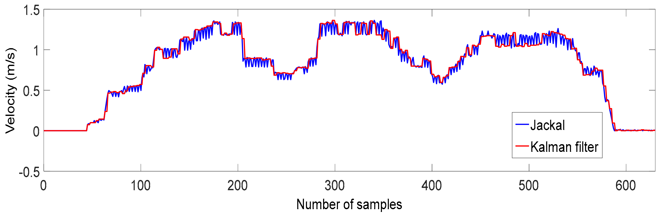
In this paper, the operation-varying threshold to be developed can be referred to as an adaptive threshold (AT) in order to distinguish it from the time-varying dynamic threshold. The adaptive threshold is critical in terms of both the adaptability to provide the robustness for automotive CPS and the sensitivity to accurately detect critical faults in the presence of anomalies. We identify a problem with respect to sensitivity and adaptability through the following simple experiment in detail. We exploit an unmanned ground vehicle (UGV) called Jackal as a target system [
27]. A new adaptive cruise control (ACC) function is implemented in the target system. The operation of the physical systems can change with time while ACC driving. For the sake of simplicity, we assume that our target system performs uniform linear motion, as the Jackal UGV continues to move on a straight line with a constant velocity. During the ACC operation, states of the moving physical system might not depend on dynamics and be linear during a certain period.
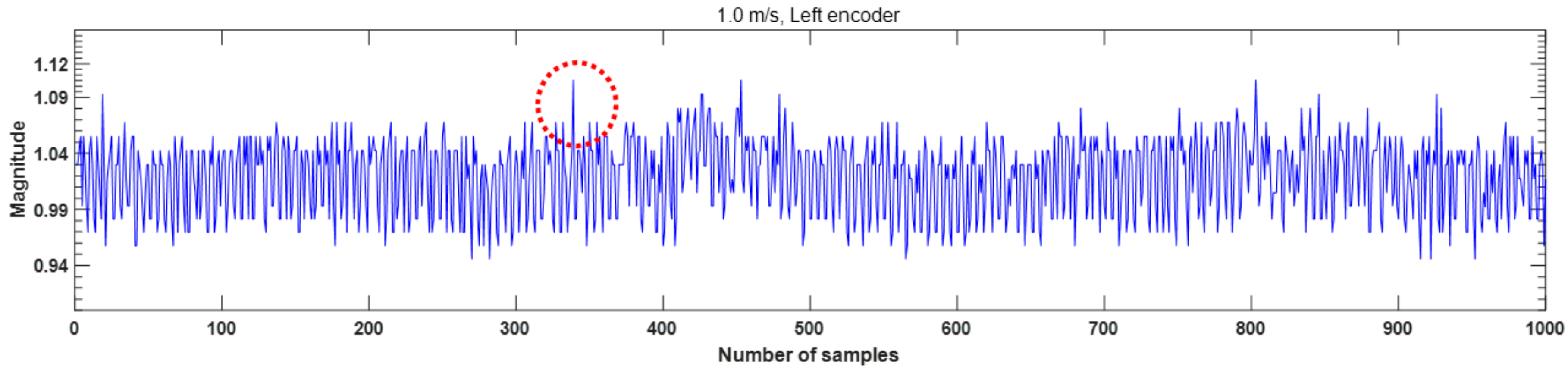
Figure 1 shows the real variables measured from a left encoder of the Jackal UGV. Although it drives on a straight line in a normal situation without any major fault of the sensors, we observe many anomalies for about 50 s. In other words, due to the environment uncertainty, we can see that there are frequently sensed data with noise while driving but they only show a small difference from the normal data.
In the existing model-based detection applied to the Jackal UGV, after the residual is generated using these measurements as shown in
Figure 1, the difference between the magnitudes of them are examined only with the fixed threshold. The cyber system, therefore, concludes that the target system may go into the abnormal state as some faults of the encoder are detected, even though Jackal is actually in a normal state. It is no wonder that a false positive rate related to these anomalies could increase dramatically over time. This is because the fixed threshold does not respond to a changing environment where some anomalies occur naturally with uncertainty while driving. For instance, using the low fixed threshold could result in misclassifying some data of normal states into data of abnormal states, which trigger a false alarm related to the false positive error. On the contrary the high fixed threshold could lead to many false negative errors. Furthermore, for the purpose of disrupting the system, if a malicious adversary injects the malicious sensing data that enters as normal into the system through the intermediate network, the malicious data cannot be distinguished from the normal data. Consequently, the system has false negative errors.
The threshold adaptive to the dynamic environment is required to accurately detect the anomalies but should be sensitive to the changes of residuals generated. Otherwise, the false errors including FP and FN errors increases. The dynamic environment involves the environment uncertainty. The changes of residuals are mainly caused by both model uncertainties.
2.2. Challenges and Our Methodology
The state of the physical system may be gradually changed with uncertainty and nonlinearity and the cumulative impact of the undetected subtle changes during the operation might be considered negative to providing safe of CPS. In order to achieve a high level of the adaptability of the system and respond to the sensitivity of the generated residual, our first idea is to approximately identify and assess normality with residual derived from the normal operation. There are numerous methods which follow a heuristic process to support approximation derived from statistical analysis of incoming data [
1,
2,
28,
29]. The normality of the system aims to differentiate between normal and anomalous data by analyzing the tendency of the residual generation patterns. At an abstract level, identifying the normality is to define a region representing the normal condition and pick out any residual which does not belong to the normal region. Only the anomalous data that are acceptable to the system are quantitatively identified through assessing normality of the physical system during the normal driving operation. However, the data with environment uncertainty affect the quality of the tendency analysis of the residual generation pattern since they seem to be similar to the actual normal data. Another issue disturbing the normality assessment is related to model uncertainty (modeling errors) and a critical challenge is to measure quantitatively the effects of modeling uncertainty. In addition, the current normal data might not be representative of the normal state after changing the operation of the system. Hence a model representing the normality of the physical system needs to be designed with some flexibility, considering a data pattern of fluctuations caused by outlier and noise related to environment uncertainty and modeling uncertainty. Note that the normality with flexibility for data cannot be obviously defined since the uncertainty distribution is unknown. We consider a number of cases for possible normality and perform statistical tendency analysis for only one input for the same physical variable (i.e., the velocity of Jackal UGV). The normality assessment should be performed for each operation of the system.
In the tendency analysis, we assume that if noise and outlier have a small magnitude as well as being infrequent, then they are negligible. The noise and the outlier are considered the normal data even if there is big difference from normal data but it does not happen often. We, therefore, focus on an anomaly frequency of data within a given period for the data obtained during the normal operation. Although the existing statistical analysis mainly requires a large amount of data, we use only a small amount of data with a certain uncertainty limited by time intervals. Through the statistical tendency analysis, we offer a new way to allow the data itself to suggest a normality model fit for its purpose, which does not assume an underlying model. In other words, rather than trying to eliminate noise and outliers for accurate measurement, we adopt a strategy using a temporary identifier when defining the normality. Accordingly, the system is provided with an acceptable region including noisy data and outlier as well as normal data.
It is reasonable that the system requires high sensitivity with respect to low modeling uncertainty and also requires high adaptability to accommodate environment uncertainty. It is, however, difficult to achieve high levels of adaptability and sensitivity simultaneously because two competitive variables are considered to determine the AT. Besides achieving high accuracy in the fault detection, a detector should raise properly an alarm for actual faults. Its performance may be captured by two results of the FPs and the FNs. The false positive indicates that the system is actually in normal operation and any fault does not occur, and the false negative indicates that the system is faulty but the cyber system does not detect any fault. Between them, the result of the latter might be a greater threat to the safety-critical CPS rather than the former. As it is known widely, there is a trade-off relationship between them. To address these issues, our key idea is to find an equilibrium point that maximizes the other’s interests without sacrificing one’s interests and achieves low type 1 and type 2 error rates. To reach an equilibrium point between two competing variables, i.e., adaptability and sensitivity, determining an optimal threshold is formulated as an optimization problem using a nonlinear programming method at each operation. By using an equilibrium point based on normality, transient faults are differentiated by picking out the soft faults from the anomalies.
4. Performance Evaluation
In this section, we evaluate the performance of the proposed fault detection method using the adaptive threshold, denoted as AT, based on the model-based method by comparing it with two dynamic thresholds. One of the dynamic threshold methods is based on root mean square (RMS) which is commonly used to generate a dynamic threshold and is denoted as RT [
30,
31,
32]. We use
RMSs for each time-window
. The other of the dynamic threshold methods is to find a knee point between the error bound and the number of fault occurrences and is denoted as KT [
1,
2,
28,
29].
We use both the training and test data as residuals which are obtained from the encoder sensors while Jackal UGV drives on the real road at each of several velocities from 0.7 m/s to 1.6 m/s by 0.3 m/s. Training data are used to generate AT for the adaptive pool as well as RT and KT. Test data are used for performance evaluation.
Table 1 lists all of the thresholds generated according to AT, RT, and KT for each velocity. However, the values of RT are not described in detail and is only mean values for each velocity
because they are different for each time-window
. In the residual evaluation, we use the
of the first threshold for differentiating the anomalous data from the normal data before the
is used as the second threshold to detect transient faults from the anomalous data. Note that the difference between the first thresholds (
) of AT and KT is the largest at the velocity of 1.3 m/s.
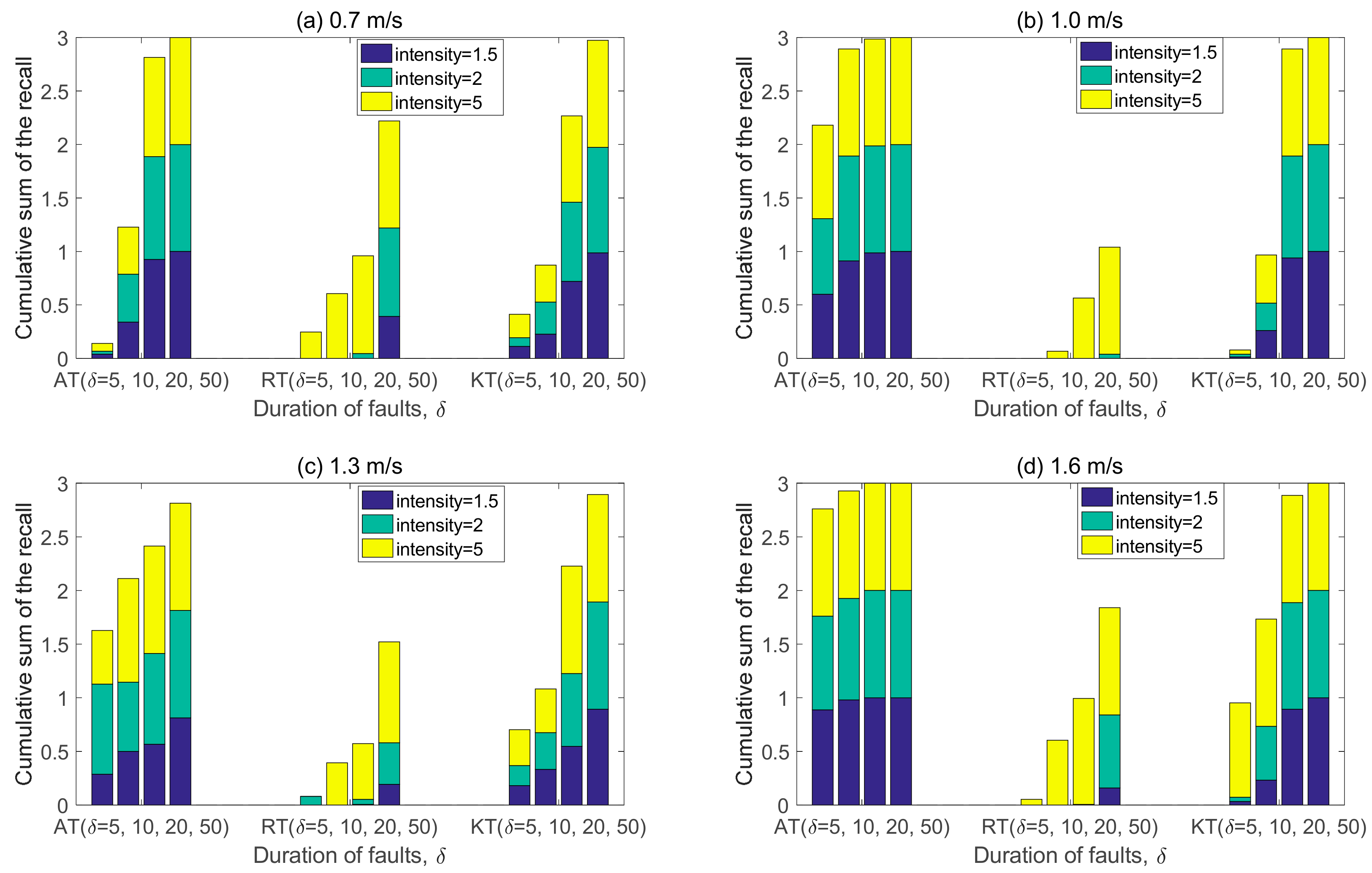
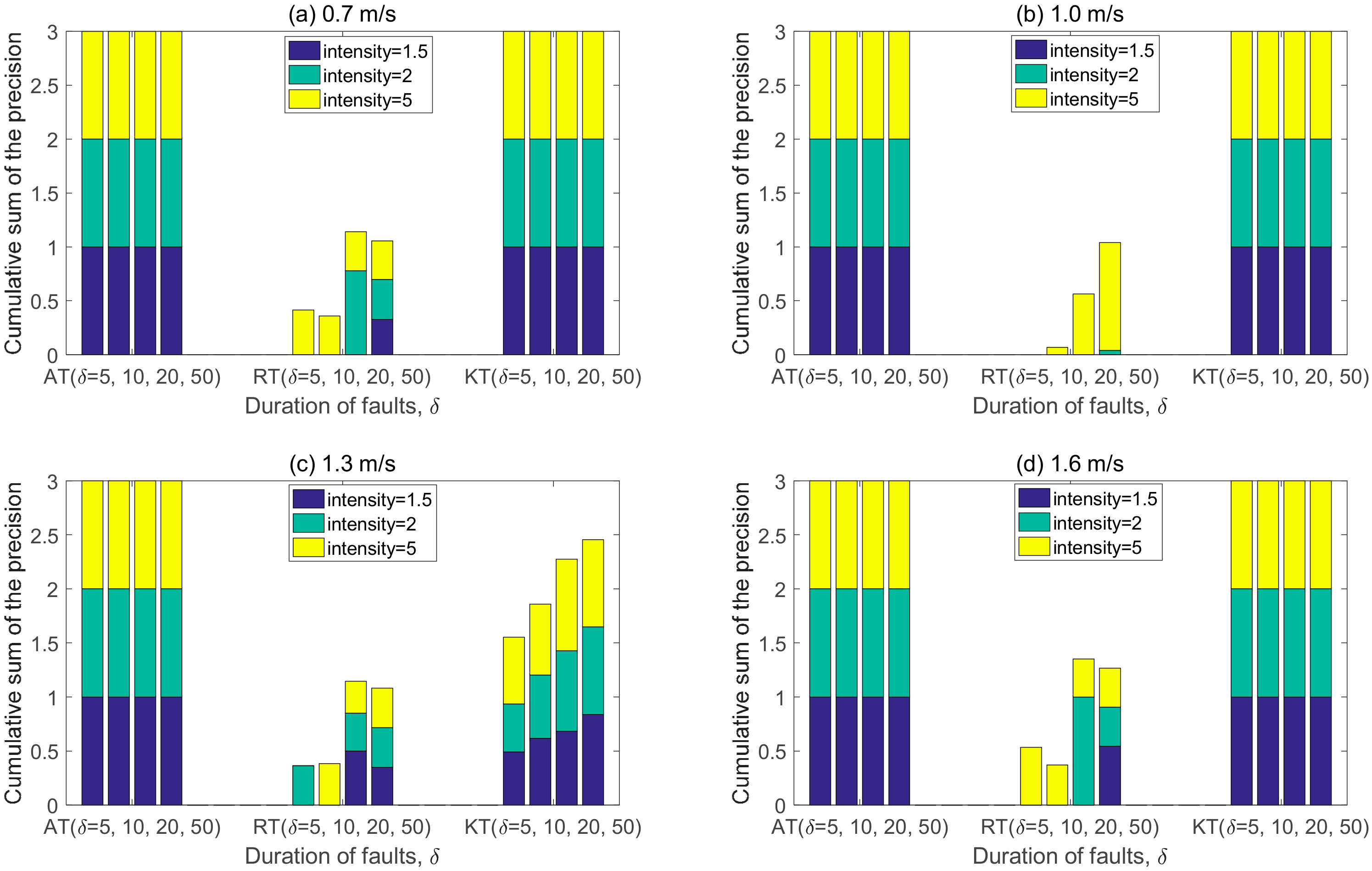
To demonstrate the high accuracy and the low type 1 and 2 errors with the change of the operation, we present the recall, accuracy, and precision as assessment outcomes when divergent scenarios are adopted. The high recall represents the low false negative error rate, which is calculated by . The low false positive rate results in the high precision which is calculated by . In our experiments, four scenarios associated with the velocity changes, and three scenarios with respect to a type of transient fault are designed. Furthermore, for each experiment, the variables for the duration and intensity of faults injected are varied. The duration and the intensity are useful to assess adaptability and sensitivity, respectively.
We inject constant, random, noise faults for performance evaluation. It is worth attempting constant faults because they show how well the adaptive thresholds basically work in accordance with the controlled environmental parameters such as the intensity and the duration of faults. The random fault detection is very meaningful in terms of how sensitive it is to identify faults similar to the original data because one value is selected from the distribution of the values of the original data and is used as a fault. Finally, the noise fault is injected with the magnitude similar to the noise which is most common and can occur in nature. It is worthwhile noting that the adaptive threshold generation is sufficient for statistical analysis of the data obtained in the normal operation.
For each experiment, the timing of fault occurrence is selected randomly and the number of fault occurrence is three, the magnitude (intensity) of the fault is always different according to types of faults. While three types of faults are injected into real measurements, the duration of faults are varied from five samples (250 ms) to 50 samples (2.5 s). The evaluation is conducted repeatedly for 50 at the given time window (i.e., = 100).
4.1. Constant Faults
Constant faults are just to add the constant magnitude to the original values. Rather than injecting several constant values selected randomly, the constant magnitudes are generated by using the predefined values for intensity in order to give consistency to the constant values. The constant magnitude is determined by using the predefined intensity and the magnitude of several samples picked randomly from the original data. Hence, the magnitude of the constant fault is the magnitude of the picked sample multiplied by the intensity plus the magnitude of the picked sample. The values of the intensity used is
= {1.5, 2, 5} [
33]. The magnitude for constant faults, denoted as
, is calculated by
where the magnitude of the data that is randomly selected is denoted as
, and
is one of the values of the intensity. From Equation (10), when
= 1.5 is applied, the constant faults with one value in the range of
] are generated by about 100% of the total constant faults where
is the mean value of the training data at the certain velocity. When
= 5 is applied, constant faults in the range of
] account for about 100%.
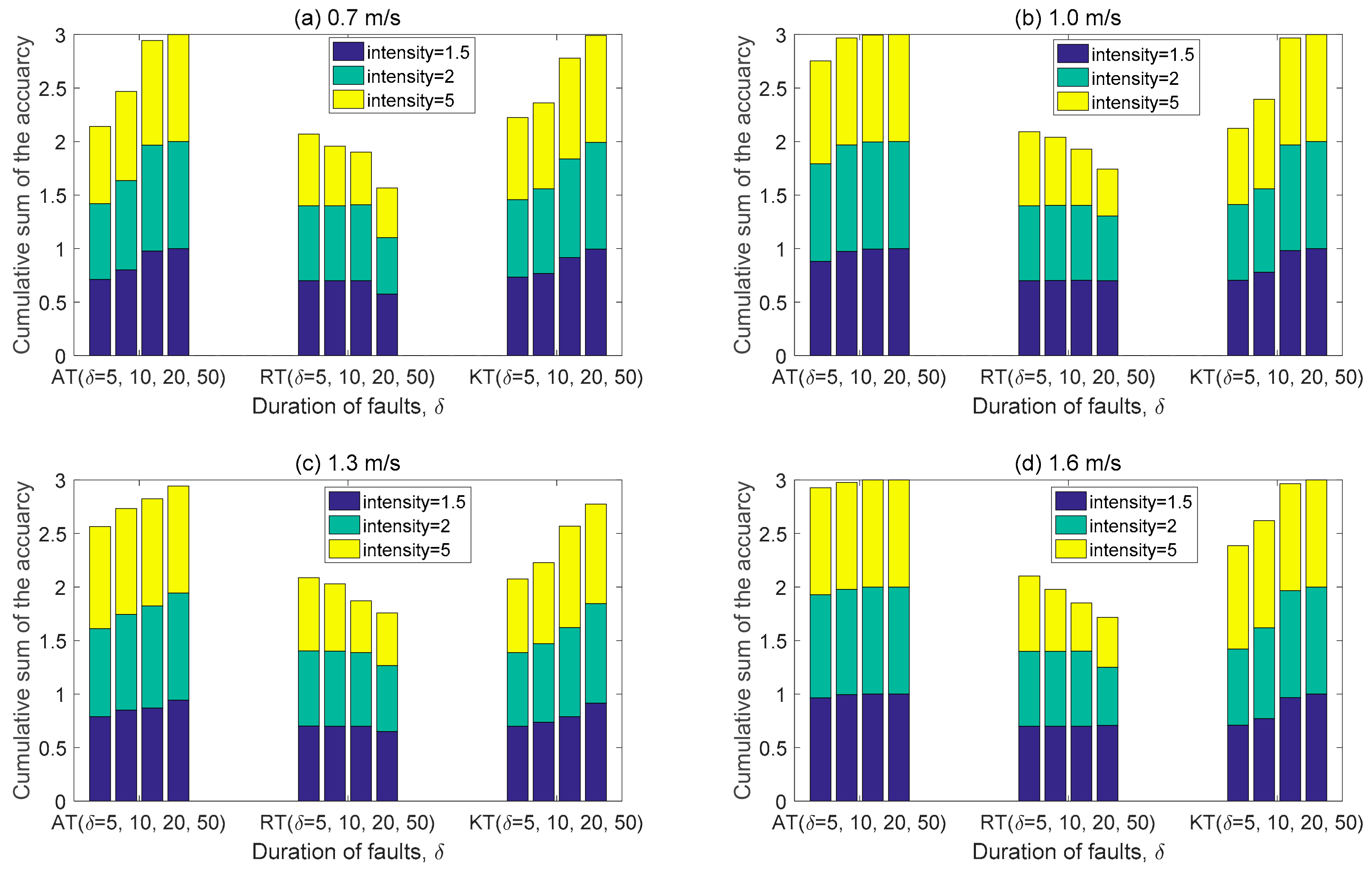
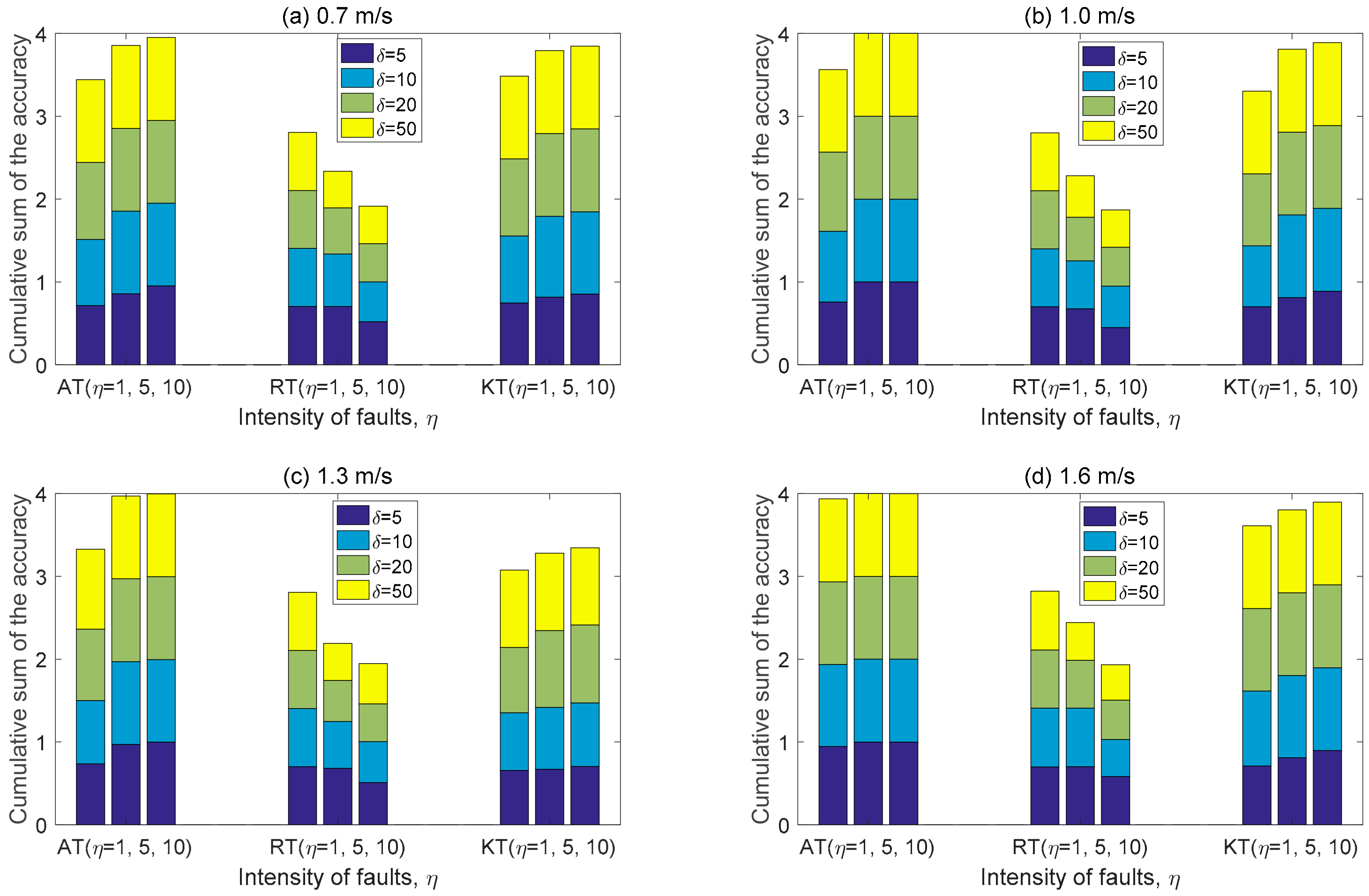
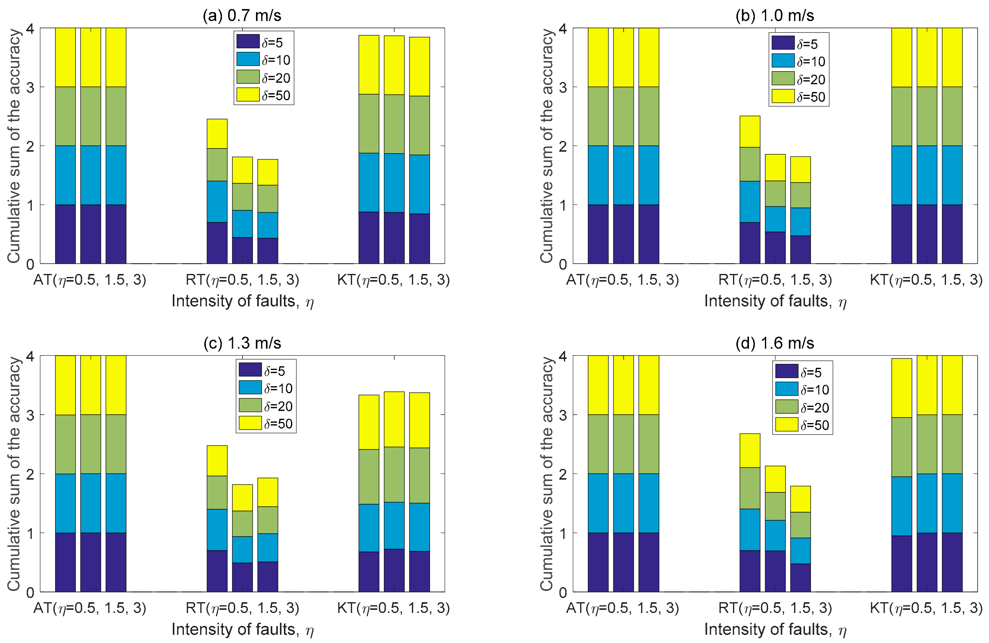
Figure 4 shows the performance results in terms of accuracy calculated by
. A true positive (TP) means a transient fault that is correctly identified, a true negative (TN) is a normal data including a soft fault that is correctly identified, an FP is an actual normal data that is identified as a transient fault, and an FN means an actual faulty data that is identified as a normal data in fault detection.
Overall, AT demonstrates better performance than RT and KT. For all velocities, it shows the trend that the performance of AT is not significantly affected by the magnitude of the intensity unlike KT and RT, and AT has also high performance level regardless of the duration as the velocity increases. Only when the duration is low ( 5) at the low velocity (0.7 m/s), the performance of AT is less than 2% (three samples) of that of KT. Under the small duration of the constant faults injected at low velocity, the acquired measurements are very small and the change (standard deviation) in the acquired measurements is not large. In this regard, the small difference between the given thresholds of (i.e., 0.117679 of AT and 0.11 of KT) seems to have a great effect on the determination of the anomalous region. Except in the case above, the performance of AT overcomes those of RT and KT performance regardless of the duration and intensity as the speed increases. Thus, our AT shows good detection results because it is sensitive to the very small intensity of injected faults.
In the case of KT, although the accuracy performance of KT shows the similar tendency to that of our AT, it notes that the accuracy of KT is highly affected by the length of duration rather than the magnitude of the intensity. For example, the performance at the small intensity ( is about 4% lower than that at the largest intensity ( = 5) at the lowest speed. In addition, at the short duration ( the performance of KT is not any the better even if the velocity increases. This result seems to be due to the high value of the second threshold which may cause an increase in FN.
Regardless of velocities, as the duration and intensity are shorter ( and smaller ( = 1.5 and 2) respectively, the RT has better performance. From these results, we find out that RT is sensitive to small changes. However, if the intensity is higher, both the TPs and FPs increase at the same time while the TNs decreases. This fact is again evident from plotting the precision.
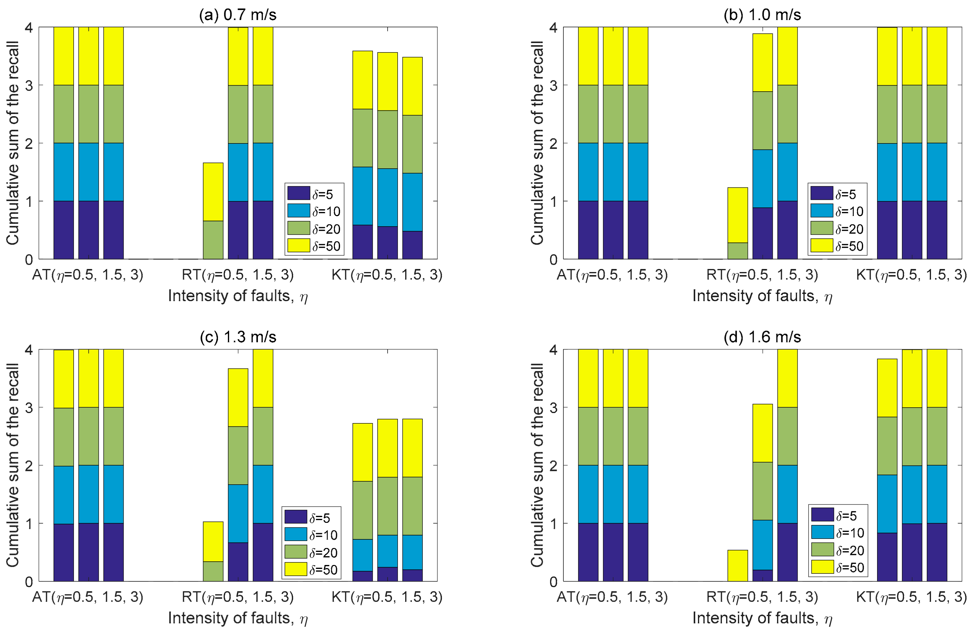
Figure 5 shows the recall presenting the relationship between TPs and FNs. As mentioned above, because our adaptive thresholds are designed for the safety-critical application, achieving the low false negatives is very important. Since the magnitude of the constant faults injected is not large, FNs tends to increase in all thresholds as the duration decreases.
In other words, such data are actually the faults although they are identified in the normal state.
Especially, RT has a significantly higher FNs and fewer TPs when the duration and the intensity are shorter and smaller, respectively, resulting in no recall or very low recall. In the case of KT, since FNs is much higher in short fault duration ( than in large duration even though the velocity increases, its recall performance is poor. This is because the shorter duration never helps determine the anomalous region by the first threshold of KT.
In AT, as the duration increases, the data to be faults within the particular anomalous region increases in the number and the detection is performed well by the second low threshold, which is more sophisticated than that of KT. As the velocity increases, the AT performance becomes more distinct because the proposed optimal thresholds are adapted well to the high uncertainty in the driving environment where the data variation is high. Only at the recall at 0.7 m/s and , the recall appears low since the FNs of AT is a little larger than those of KT. This seems to be due to the wide normal region because the first threshold of AT is slightly larger than that of KT when its velocity is the slowest.
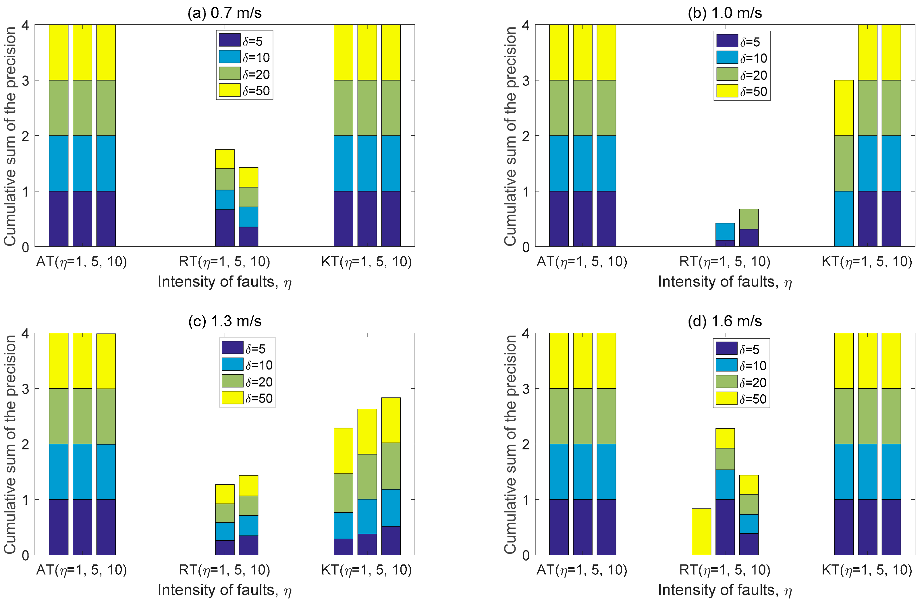
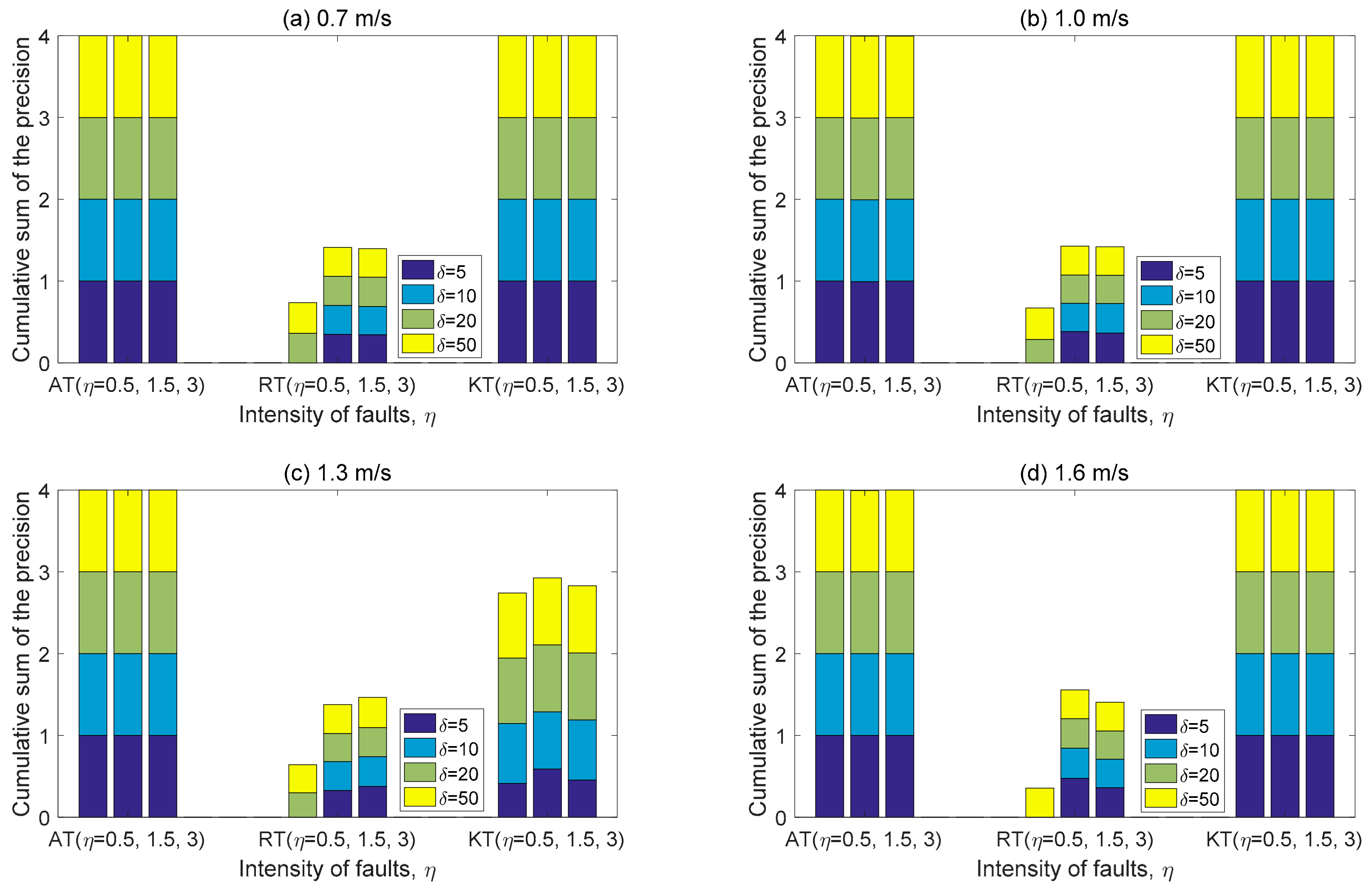
The precision with regard to false positives is shown in
Figure 6. Both AT and KT which show 0% of the FP rate for all velocities conduct the elaborate detection of faults from the anomalous region. As mentioned earlier, in the case of RT, both FPs and TPs are increased at the same time as the intensity is larger and the duration is longer. On the contrary to this, RT does not respond to the small changes to which the intensity and duration are applied with the low values.
4.2. Random Faults
The magnitude of random faults injected in our experiments is determined by using one value selected randomly in the distribution of the magnitude of the original data at each velocity. The duration variation follows that of the constant fault. The intensity is by which the selected magnitude is multiplied. The magnitude of random faults is given by
where is a random number drawn from the standard normal distribution, is one of the intensity values, and and are the mean value and the standard deviation of the training data at the certain velocity respectively.
The accuracy of the random fault detection is presented in
Figure 7. At all velocities except for 0.7 m/s of the velocity, AT achieves the best performance close to 100% when exceeding the intensity of a certain magnitude (
. As with constant faults, AT has lower performance than KT only in the shortest duration and velocity (
and it seems to be due to the slightly high threshold of AT at the lowest velocity. From Equation (11), when
= 1 is applied, the random faults with one value in the range of
] are generated by about 47% of the total random faults and random faults in the range of
] account for about 82%. Hence, when
= 1 is applied, these results are so meaningful in terms of sensitivity to small changes. The ability to identify them is superior at all velocities compared to other methods when the faults with the magnitude similar to that of the original data are injected. Obviously, the larger the intensity is, the closer to 100% the performance of AT is.
Unlike AT, the accuracy of KT is significantly influenced by the intensity and duration irrespective of the velocity. Furthermore, when = 5 and 10, although the magnitude that goes beyond the value of account for about 47% and about 71% of the total faults generated, respectively, the performance of KT is not as good as that of AT. RT tends to decrease in the performance as the duration and intensity increase. In the case of RT, when the intensity is small ( = 1), the TPs do not increase regardless of the duration, but the actual normal data are identified well. When the intensity is medium and high, the TPs increase but the ability is insufficient for identifying the actual normal data as the duration increases. Therefore, these results mean that KT and RT are not adaptive and sensitive even though they are determined dynamically.
Figure 8 shows the results of the recall of three methods. It is similar to the tendency of the accuracy of both AT and KT except RT. When the velocity is 0.7 m/s, the recall performance is low as the duration becomes shorter. This is due to the increase in the occurrence of FNs, that is, the faults are mistaken as normal data. The cause of the FN increase seems to be closely related to the size of the time window. However, from the results, we find that this tendency shows that AT adapts quickly as the intensity becomes stronger. At the velocity above 1.0 m/s, we also find that AT and KT produce many FNs only when
= 1. However, the frequency of FNs in AT is much smaller than that of KT even though the duration is very short.
Furthermore, as the intensity and the velocity increase, AT does not generate any FN error, but KT still has many FN errors. In the random faults, RT is unable to detect faults with similar size to the original data, and classify almost all injected faults as normal data. However, the intensity and duration become larger, the amount of mistaken data become less. In the case of RT, when the intensity is small ( = 1), the FNs increases regardless of the duration but no faults are detected. When the intensity is medium, the FNs decreases as the duration increases. The FN frequency is very low when the intensity is high and the duration is small. Only when the intensity is large enough to identify the difference, the RT is applied to detect faults.
The precision results of each method are shown in
Figure 9 according to the magnitude of intensity. At all velocities, AT shows the best performance and 0% of FP occurrence. At 1.0 m/s and 1.3 m/s, there is a significant difference in performance between AT and KT. The difference between the two thresholds at all intensities seems to make an appreciable difference to the performance. As mentioned above, the difference between the first thresholds (
) of AT and KT is the largest at the velocity of 1.3 m/s. Since the small threshold of KT, compared to that of AT, results in the wide anomalous region, in random faults, KT shows low performance with many FPs that occur constantly for all conditions. In contrast, AT does not have any FP at all. At 1.0 m/s, since the second threshold (
of KT is too high, KT fails to detect the random faults under the lowest intensity (
= 1) and the shortest duration (
. In the case of RT, the performance is better as its velocity increases but the precision is very low. The intensity and the duration are higher simultaneously, a large number of FPs also occurs while TPs are increased. Especially, when the injected faults are similar to the magnitude of the original data (
), the detection performance is zero since almost all injected faults are classified as normal data. This is because all, including the normal and anomalous, data are identified as the normal data when
.
4.3. Noise Faults
In our experiment, injecting noise faults aims to assess the detectability under Additive Gaussian white noise (AGWN) that is most common in communication systems and can occur in nature. This fault is generated by adding the one value drawn from in a zero-mean normal distribution with a given variance to the magnitude of the original data at each velocity. The performance can be bound to vary on the given variance, but for the purpose of noise faults involved in these experiments, the variance is fixed at one. The duration variation is the same as that of the constant and random faults. The magnitude of noise faults is determined by:
where
is a random number drawn from the standard normal distribution, and
is one of the intensity of
. This intensity used is quite different from those of the random faults and was already used in the research of SHARMA et al. [
25]. From Equation (12), when
= 0.5 is applied, the noise faults with one value in the range of
] are generated by about 0% of the total noise faults where
is the mean value of the training data at the certain velocity, and them in the range of
] account for about 100%. Note that the magnitude of noise faults is much larger than that of random faults.
Figure 10 shows the detection accuracy of the three thresholds for noise faults. For all velocities, AT has the precision of 100% and is not affected by the duration and intensity. KT shows that its performance is mainly low at the shortest duration and the lowest intensity for all velocity when it is compared to other conditions. From these results, we discovery that KT is less sensitive to the trivial noise. Although KT has the worst performance at 1.3 m/s for the noise faults, the performance of the noise faults is increased slightly more than that of random faults. In the case of RT, the accuracy is better when the intensity is smaller and the duration is shorter. However, it can be predicted that many FPs can occur since it responds sensitively to small changes. This remark can be seen in the graph of precision.
In
Figure 11, we present the results of recall at each velocity. We can see that in AT, no FN has occurred for all velocities. In the case of KT of 0.7 m/s, the FNs occur unconditionally when the duration is 5 for all of the intensities. Even as the velocity increases, the sensitivity to small changes is still low when the duration is short. It indicates that KT is not capable of responding to the very short occurrence of noise. In KT, the levels of intensity have little effect on the noise fault detection since the magnitude of the noise faults is already too large as mention above. As with other faults, the recall of KT is the worst at 1.3 m/s, and FNs increases at both
regardless of the intensity, since the lower first and the high second thresholds influences are still on it.
In case of RT, the recall is better than that of KT at 0.7 m/s and is comparable to that of KT except for 0.7 m/s when the intensity is high (). From this graph, we can find that RT has the ability to detect faults better than KT in the case of noise with a magnitude of a certain level (.
Figure 12 depicts the results of precision. From these results, it can be seen that AT is well adapted to the large changes from the small changes by using the proposed thresholds for all velocities, and any FP has not occurred at all.
In the noise faults, except for 1.3 m/s, as KT does not have FPs, its precision achieves 100%. However, at 1.3 m/s constant FPs occur regardless of the intensity and the duration, but TPs increase as the duration becomes higher. In addition, KT at 1.3 m/s shows better precision than KT in random faults. This is because the magnitude of the noise faults is large enough to be detected even though the intensity for them is the lowest (. Nevertheless, the FPR (false positive rate) of the KT is in the range of about 58% to about 18% at 1.3 m/s. In RT, the FP is increased significantly as the duration increases at the certain levels of intensity (. When the intensity is below 1.5, RT is not capable of detecting noise faults.
4.4. Discussion
The FNR (false negative rate) and FPR of the experimental results for all scenarios are averaged and shown in
Table 2. Note that the magnitude of injected faults is the smallest in constant faults and the largest in noise faults. Random faults are distributed in all ranges of the magnitude according to the intensity. For all types of faults regarding all of the intensity and duration AT does not generate any FP for all velocities, but KT does show an average 27% of FPR only at 1.3 m/s. RT shows about 64% FPR for all faults regardless of velocity.
AT shows 0% FNR for all velocities in noise faults but it has mean 7% FNR for random faults, and mean 12% FNR for constant faults, respectively, except for 0.7 m/s. KT show about 10%, 29.5%, and 38% FNR for noise, random and constant faults, respectively, except 0.7 m/s. RT not only has about 52.3% and 78.5% FNR, respectively, except 0.7 m/s for random and constant faults, but also, about 27% FNR is shown for noise faults. The reason for the poor FNR performance for constant fault injection for all thresholds seems to be that the designed intensity is too small to be distinguished from normal data and transient faults.
From the above results, we demonstrate that the AT has enough sensitivity to small changes and adaptable to various changes and has the dependability enough to support the safety for CPS. However, the performance of the AT is degraded only at both the lowest velocity and the shortest duration, probably because the variation and the values of the original training data are too small to identify the differences in the large time-window size at the lowest velocity. There is a need for further investigation related to the size of time window as the velocity slows down, which needs to be made smaller than = 100.
5. Conclusions
The critical faults have high potential to threaten the safety of automotive CPS. In particular, the transient faults in the anomalous data causes the unexpected behavior of the system during operation; however, their effects might not appear immediately. In this paper, in order to drive CPS into the stable state and to perform the operations of automotive CPS safely by detecting transient faults, we have developed a novel way to determine the adaptive threshold as the equilibrium point between competing variables. In the experimental evaluation using the real UGV data, our threshold yields a significantly better accuracy, recall, and precision than RT and KT. Against noise faults, AT shows nearly 100% accuracy, recall, and precision at each of the operation, regardless of the intensity and duration of faults. Under the constant faults, it achieves the accuracy from 85.4% to 100%, the recall of 100% from the lowest 54.2%, and the precision of 100%. AT also gives the accuracy of 100% from the lowest 83.2%, the recall of 100% from the lowest 43.8%, and the precision of 100% against random faults. In this regard, we have demonstrated that the proposed generation method enables adaptive thresholds to enhance the adaptability and sensitivity to the various environments and modeling errors and achieves a high level of detectability simultaneously in fault detection.
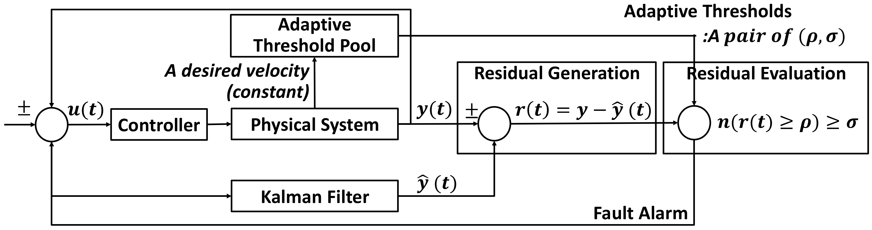
Since our method is based on the model-based detection that performs both residual generation and evaluation, the dynamics of the targeted physical system as one of automotive CPS is first modeled and is integrated into the Kalman filter to estimate the state of the physical system and generate the residual. Furthermore, we design a structure that adds the adaptive threshold pool to the basic structure of the model-based detection and extracts the pair of thresholds from it according to the referenced velocity. In order to cope with fluctuations caused by noise, environment uncertainty, and modeling uncertainty, the normality of the physical system needs to be considered with some flexibility and it also needs to find out optimally how to determine an adaptive threshold which plays an important role in distinguishing faults from anomalous data. In our approach, since the normality cannot be obviously defined due to lack of prior knowledge of the fault occurrence, we should consider many different possibilities of normality by examining the residual under normal driving conditions. By statistical analysis, the normality is assessed in order to define the normal and anomalous states from the data obtained under the normal operation of automotive CPS. The specified normality model allows us to get various pairs of thresholds that can be used to detect transient faults in the residual evaluation. We find out one optimal pair achieving the best performance required by CPS as the adaptability and sensitivity are considered to minimize uncertainties of modeling and environment. To do this, after the performance measures that can represent two comparable variables are defined, the optimization problem is formulated by using the nonlinear programming method in order to maximize the interests of two measures.
These experimental results show that there is an obvious difference among the performance results of three thresholds. In terms of accuracy, recall, and precision, performance evaluation of our AT is performed based on various scenarios, compared with the performance of other dynamic threshold techniques. When the performance is analyzed by varying the duration and intensity for three kinds of faults, AT generated by the proposed method is not influenced by the change of the intensity and duration at each velocity. KT could not detect faults properly if the intensity is low or/and the duration is short. Since RT is sensitive to small changes of measurements, its performance is significantly changed according to duration and intensity and showed similar performance regardless of velocity.
The AT method helps prevent misleading interpretations that the cyber system concludes some intermittent anomalous data and noises as fatal faults even though they occur naturally, disappear soon, and do not affect adversely the control of the system. AT is not only competent to diagnosis the faults with high levels of sensitivity and adaptability, but also it achieves good performance with only a small amount of data with a certain uncertainty limited by time intervals. In particular, it is noteworthy that the thresholds are optimally determined in response to the obtained measurements that change significantly as the velocity is varied because it proves that the intensity and duration have nothing with the performance of AT. Therefore, the adaptive threshold generated from the combination of our threshold generation method and the normality model can be a good criterion for distinguishing between normal and anomalous states as well as detecting faults. The AT determined from the equilibrium can be said to have high degrees of adaptability and sensitivity. In future work, at lower velocities, the performance of AT needs to be improved by varying the time window size.


