Modeling and Solution of the Routing Problem in Vehicular Delay-Tolerant Networks: A Dual, Deep Learning Perspective

Abstract

The exponential growth of cities has brought important challenges such as waste management, pollution and overpopulation, and the administration of transportation. To mitigate these problems, the idea of the smart city was born, seeking to provide robust solutions integrating sensors and electronics, information technologies, and communication networks. More particularly, to face transportation challenges, intelligent transportation systems are a vital component in this quest, helped by vehicular communication networks, which offer a communication framework for vehicles, road infrastructure, and pedestrians. The extreme conditions of vehicular environments, nonetheless, make communication between nodes that may be moving at very high speeds very difficult to achieve, so non-deterministic approaches are necessary to maximize the chances of packet delivery. In this paper, we address this problem using artificial intelligence from a hybrid perspective, focusing on both the best next message to replicate and the best next hop in its path. Furthermore, we propose a deep learning–based router (DLR+), a router with a prioritized type of message scheduler and a routing algorithm based on deep learning. Simulations done to assess the router performance show important gains in terms of network overhead and hop count, while maintaining an acceptable packet delivery ratio and delivery delays, with respect to other popular routing protocols in vehicular networks.

1. Introduction

As urban environments have exponential grow, smart cities (SC) is the technological paradigm that aims at providing the ultimate solution to the urban development in every aspect in wide areas such as social management, security and safety, health and medical care, smart living, tourism, and transportation, with the aid of sensors and electronics, communication networks, and information technologies [1,2]. Among the essential needs and key components of a smart city are intelligent transportation systems, which seek to provide a solution to transportation-related problems, such as pollution, traffic congestions, and accident reduction [3,4]. In this sense, vehicular networks play a key role by providing a communication framework for moving vehicles, road infrastructure, and pedestrians [5]. The main goal of vehicular networks is to provide seamless wireless communication between cars (vehicle to vehicle, or V2V), infrastructure (vehicle to infrastructure, or V2I), pedestrians (vehicle to pedestrian, or V2P), and virtually any object (vehicle to anything, or V2X), which would allow important improvements to transportation services as we know them as well as the creation of new ones [6,7].

The promise of vehicular networks is the evolution of transportation areas such as security and safety, traffic management, sustainability (green transportation), and other digital services, including e-commerce and infotainment, to more efficient ones. However, due to the harsh conditions of vehicular environments, this kind of network presents serious challenges that limit and slow down its deployment and adoption. For instance, the very high speeds at which nodes can move lead to a lack of end to end connectivity between them, which makes having a fixed network topology rather difficult [8]. Furthermore, the frequent disruptions in the connections add significant drawbacks in the network performance, such as poor delivery rates and long delays [8] (that is why these networks are often referred to as vehicular delay tolerant networks, or VDTN, for short). These and other issues are mainly caused by network partitioning, which in turn can be a result of several factors. Disruptions in the network can be caused when node density is sparse or very high in small areas; also, data congestion and of course the high mobility of nodes are two of the main causes of network partitioning [9]. As a consequence, delays are an expected, natural characteristic observed in the delivery process, due to the lack of an end-to-end path between source and destination, that has to be created over time with the aid of opportunistic encounters with other nodes [10]. Moreover, in order to increase the chances of delivery, copies of the messages are spread through the network in the hope that they eventually get to their destination, but this introduces another issue in the process, called network overhead. This parameter refers to the redundancy of information in the network, such as message copies that did not make it to their destination but did use network resources [10]. These particular characteristics bring to life one of the main challenges in vehicular communications, which is the message routing [10,11,12]: Depending on the application scenarios, it is desirable to have a high delivery ratio, while maintaining acceptable delivery delays and network overhead. Packet routing in these environments is a difficult situation to solve, as no predefined paths in the network can be considered, so deterministic methods for optimization tend to fail and non-deterministic approaches have to be employed instead [10,12]. To face this issue, VDTN routing algorithms opportunistically rely on other nodes to deliver data packets using the store-carry-forward mechanism, where nodes store exchanged data with other nodes, carrying it as they travel and forwarding it when appropriate, in the hope that the messages make it to their destination.

In the past several years, many opportunistic routing algorithms and non-deterministic solutions have been proposed [13,14], but due to the very unique characteristics of this kind of networks, the efficiency is limited, and the search for the best algorithm that can provide seamless and reliable communication is still an ongoing primary quest. Some algorithms, like the epidemic routing [15] and spray and wait [16], make use solely of a flooding-based principle, in which copies of the message to deliver are spread in a controlled way. Others, like PRoPHET [17], make use of probabilistic encounters maximizing the chances of two nodes meeting in the future. One third group, like SeeR [18], seeks to make use of heuristic approaches to approximate a global optimization in a larger search space. Nowadays and for the past few years, artificial intelligence (AI) has become an increasingly important field of study to assist in the evolution of science, engineering, business, medicine, and more [19]. Industry, finance, healthcare, education, and transportation have seen important advances with the aid of image and speech recognition, natural language processing, and intelligent control and predictions [19,20,21], which are possible thanks to different AI techniques. In this paper, we propose DLR+, a deep learning–based router that is capable of learning to make intelligent decisions based on local and global conditions from a dual perspective. The simulation results show that this router outperforms some well-known routers in network overhead and hop count, while maintaining an acceptable delivery rate.

The rest of the paper is organized as follows: In Section 2, we dive into relevant related work, and in Section 3, we frame the routing problem in a more formal way. In Section 4, an overview of the proposed router is given, presenting the router architecture and its modules, and in Section 5, we describe the routing algorithm in more detail. Section 6 is dedicated to the experiment and in Section 7, we discuss the obtained results. Finally, in Section 8, we conclude this paper, providing a quick summary of this work and the findings, and provide some recommendations to further advance on this topic taking the proposed router as a starting point.

2. Related Work

In the past several years, several approaches have been proposed to address the routing problem in VDTN, but due to the particular characteristics of vehicular environments, and especially the lack of an end-to-end connection between nodes in a vehicular network, non-deterministic approaches must be used [10,11].

Some routers for delay-disruption tolerant networks, like the epidemic router [15] and the spray and wait router [16], use a flooding-based principle of spreading copies of the messages to newly discovered contacts. The epidemic router is one of the most popular routers in this category [7,15], whose approach is to distribute messages to other hosts within connected portions of the network, relying upon such carriers coming into contact with another connected portion of the network through node mobility, hoping that through that transitive transmission of data, messages will eventually reach their destination. This routing protocol provides an acceptable delivery rate and delay but at the expense of using too many resources in the network. In the same way, the spray and wait router [16] uses a similar (flooding-based) but more controlled mechanism, “spraying” a number of copies into the network, and “waiting” until one of these nodes meets the destination. More particularly, this router passes $L$ copies from the source node (phase 1—spray), and then each of the $L$ copies waits in their temporal host until there is a contact, if any, with the destination (phase 2—wait), to whom they are only then forwarded.

Other routers use probabilistic approaches to increase the chances of packet delivery. MaxProp [22] is one of the first routers proposed in this category. This router uses what the authors call an estimated delivery likelihood for each node in the network, updated through incremental averaging, so nodes that are seen infrequently obtain lower values over time, and packets that are ranked with the highest priority are the first to be transmitted during a transfer opportunity, whereas those ranked with the lowest priority are the first to be deleted to make room for incoming packets. On the other hand, the PRoPHET Router [17] is perhaps the most popular router in the probabilistic routing category. Based on the history of encounters between the nodes, this router introduces a metric called delivery predictability, a set of probabilities for successful delivery to known destinations in the network and established at each node for each known destination. This way, when nodes meet, they exchange information about the delivery predictabilities and update their own information accordingly, and the final forwarding decision is made based on these values to whether or not pass the current message to particular nodes.

In recent years, the use of artificial intelligence techniques has gained tremendous popularity because of the successful application to many practical optimization, prediction, and classification problems that include image processing (facial recognition, cancer detection, etc.), forecasting (stock prediction, weather forecasting, etc.), and others [23,24]. The application of AI-based algorithms to the routing problem in VDTN, however, is still not fully explored, although some efforts have been conducted towards this direction. In this category, SeeR is one of the most efficient routers [18]. This router uses the simulated annealing algorithm to evaluate which messages are best to be transferred in each contact opportunity. Each message is associated with a cost function in terms of the hop count and the average intercontact time of the current node, and one node transfers a message to another node if the second node offers lower cost value. Otherwise, the messages are forwarded, first decreasing their probability. Their experiment results show considerable gains in the average delivery ratio and improvements in delivery delays with respect to flooding algorithms like epidemic routing and spray and wait. Another router in this category is KNNR, a router based on the KNN classification algorithm, proposed in [25]. They use six parameters (available buffer space, time-out ratio, hop count, neighbor node distance from destination, interaction probability, and neighbor speed) to decide on the final label. The class used during the training stage (which is done offline) is based on the interaction probability, which is the same used in PRoPHET. Like SeeR, this router addresses the routing problem under the best next message perspective. Their results show better average delivery ratio and acceptable delay with respect to Epidemic and PRoPHET routers. Also, the authors in [26] propose MLProph, a machine learning model as a routing protocol. They use the PRoPHET router as the base and expand its capabilities by adding some other features to the equation, and the result is an improved router with respect to the base. Although they use a neural network model as well, they use a different algorithm than the one proposed here, Furthermore, their router makes calculations for each connected router, which increases computational resources such as time and CPU usage, and transfers sensible information from the connected nodes, increasing the risk of security leaks. In [27], the authors presented CRPO (cognitive routing protocol for opportunistic networks), which also uses a neural network as the core, although the decision parameter is the probability of encounter defined in PRoPHET; hence, CRPO is similar in nature to MLProph, since both of them use PRoPHET’s probability as their main decision parameter. Although the authors claim that the training stage is run for X units of time each Y units of time, they do not provide further detail on this. Finally, in [28], the authors explore the possibility of removing the routing protocol from a wireless network using deep learning techniques. The problem statement, however, is formulated as a classical optimization problem to find the shortest path in a connected graph. That is, the scenario is different to that of a vehicular network, since one of the main characteristics in VDTN is precisely the lack of a fixed topology with pre-defined paths.

3. Formulation of the Routing Problem

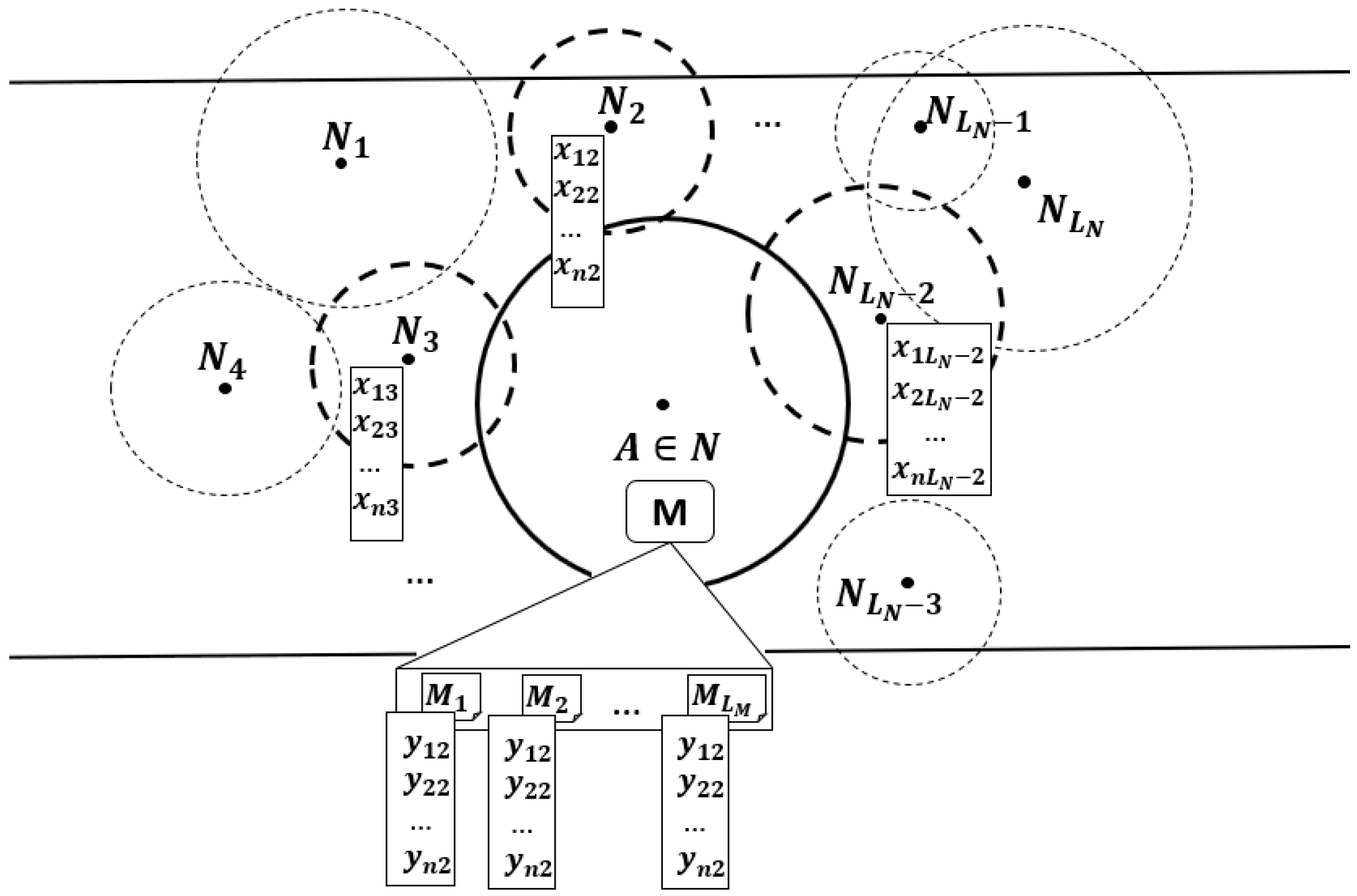
Let $N=\left\{N_i\right|1\le i\le L_N\}$ be the set of available nodes in a vehicular network with constant disruptions and non-fixed topology, and let $A\in N$ be a given node in that set (Figure 1). Given the fact that there are no predefined paths and the connections are intermittent, the nodes in the network must act opportunistically, taking advantage of any node that gets into their communication range, because whenever these encounters happen, the opportunity of replicating a message arises. In those situations, $A$ has to decide on a node to start a transfer, and several criteria can be used for this decision, but ultimately, $A$ would like to choose the node with better capabilities of further spreading the messages until hopefully they get to their destination. Following this approach, the routing problem can then be expressed as finding the best next hop (BNH) for the messages. That is, from all $k$ nodes that $A$ is connected to in a given moment, the one, $N_x$, with better fitness $f_x$ must be determined, in terms of its current features $x_1,\dots x_n$. Furthermore, in order to optimize the communication conditions, not only must the best next hop $B$ be selected, but we can also detect the best next message (BNM) to be transferred. That is, based on its current attributes $y_1,y_2,\dots , y_m$, we must be able to select from the message queue $M=\left\{M_i\right|1\le i\le L_M\}$ the message $M_y\in M$ with the best fitness $f_y$. Because neural networks have the power to learn very complex non-linear patterns, they are the perfect fit for what we are traying to achieve here, so we can model both optimization scenarios as binary classification tasks to allow us to quantify the capabilities of such nodes $N_i$ as a function $F$ of some of their characteristics $x_i$ as $f_x=F\left(x_1,x_2,\dots x_n\right)$ and the capabilities of such messages $M_i$ as a function $G$ of some of their characteristics $y_i$ as $f_y=G\left(y_1,y_2,\dots y_n\right)$.

4. DLR+ Router Overview

In this section, we describe in more detail the fundamental principle and architecture of DLR+, the router in the proposed solution. The main idea is to have a router capable of learning from the conditions of its environment and use such information to make smart forwarding decisions. In order to achieve that, the router uses two pre-trained feed forward neural networks to process the information from both its neighbors and the messages in their queues in real time and select from them the best next hop for the best next message, according to their current fitness. More details are given in the following subsections.

4.1. Router Architecture

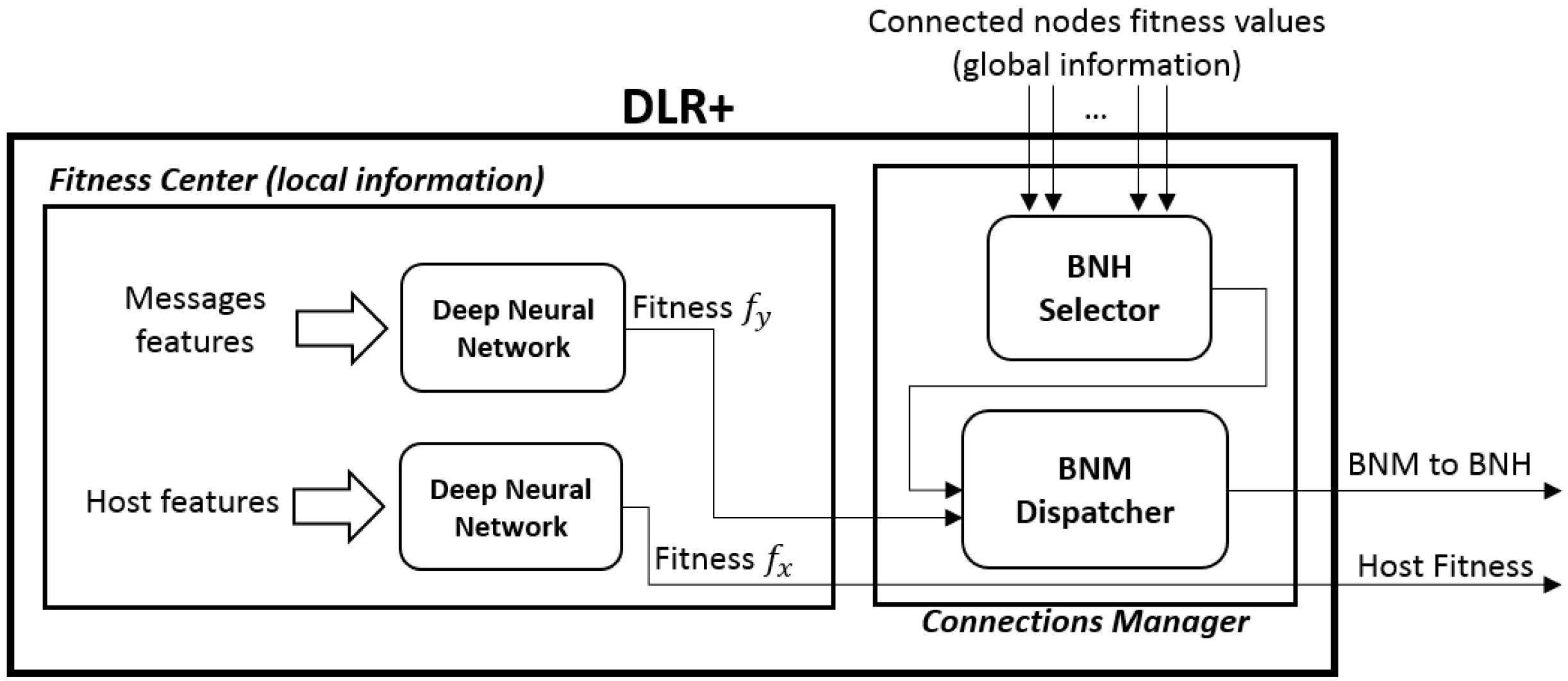
The core of the router has two fundamental modules that allow the router, upon a connection-up event, to choose the best next hop from its current connections and the best next message to send from its queue, but also to share information to other nodes (upon request), so they can decide whether or not to pass a packet to it. Such modules are called, respectively, the connections manager and the fitness center, which in turn has two independent modules for the messages and for the host itself (Figure 2).

4.1.1. The Fitness Center

This part of the router has two pre-trained deep feed forward neural networks that use the available local information to compute the router’s current fitness $f_x$, defined as the value that determines its ability to correctly deliver data packets to the final destination, and the fitness $f_y$ for each message in the queue, with $f_x,f_y\in R,0\le f_x,f_y\le 1$. The closer these values are to 1, the fitter their owners are. More details on how to get these numbers are given in Section 4.2. These values are automatically updated in each router right after a connection is ended and right after a new message has been received, so they are available and ready to be used at any moment.

4.1.2. The Connections Manager

The function that this module has is vital in the selection of the best next message for the best next hop. This module manages the incoming connections, requesting their $f_x$ values in order to select the fittest node. After this, if available, the message scheduler will send the fittest message to such node.

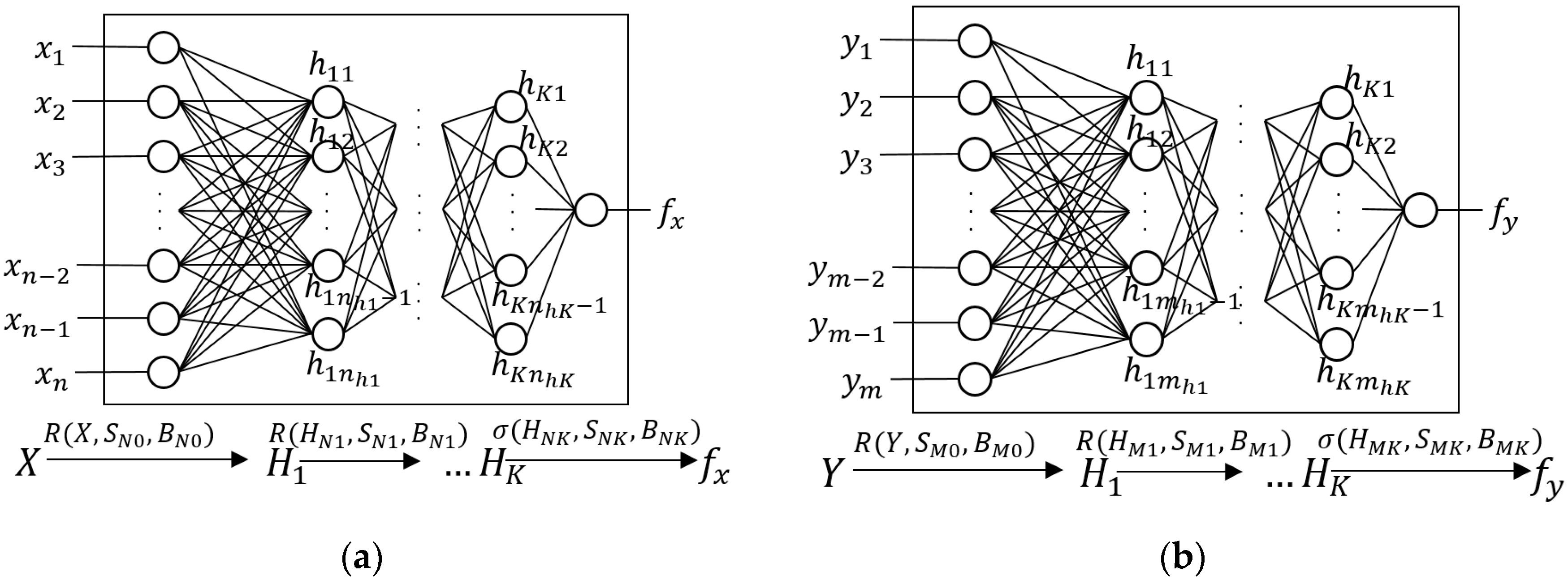
4.2. The Neural Networks

We treat the problem of finding the BNH and BNM as binary classification problems, given that we would like to know if the node and messages are in best conditions (i.e., fit) to carry and deliver the messages, or not. Thus, the neural networks used in the fitness center are feed forward neural networks, whose general architecture is presented in Figure 3.

Here, $X\in R^n$ is the set of $n$ input values $x_i, \forall i\in \left\{1,2,\dots ,n\right\}$ that reflect some of the characteristics of the host at that moment, such as its speed and buffer occupancy; $H_i\in R^{n_{hi}}$ is the vector that contains the values $h_i$(computed according to Equation (3)) of the $n_{hi}$ neurons in the hidden layer number $i,\forall i\in \left\{1,\dots , K\right\}$, where $K$ is the number of hidden layers in the network; and $f$ is the resulting fitness value of the host in the given conditions. The set of weights (synapsis) of the neural network, without its bias values, is given by $S_{N0}\in R^{n\times n_{h1}}$ for the connections between the input layer and the hidden layer 1, and $S_{Ni}\in R^{n_{hi}}$ for the connections between the hidden layer $i$ and the next hidden layer $i+1$, for all $1\le i\le K$, including the connections from the last hidden layer to the output layer. Finally, the bias values of each synapsis are given by $B_{Ni}\in R^{n_{hi}}, \forall i\in \left(0,K\right)$. Similarly, $S_{M0}\in R^{m\times m_{h1}}$ is the synapsis vector for the connections from the input layer to the first hidden layer, and $S_{Mi}\in R^{m_{hi}}$ are the synapsis for the connections from the $i$-th hidden layer to the next one, including the connections from the last hidden layer to the output layer, and the bias values of each synapsis are given by $B_{Mi}\in R^{n_{hi}}, \forall i\in \left(0,K\right])$.

As for the number $K$ of hidden layers, the universal approximation theorem [29] establishes that “a neural network with a single hidden layer with a finite number of neurons can approximate any continuous function on compact subsets in $R^n$”; this implies that, finding the appropriate parameters, a neural network with one single hidden layer is enough to represent a great amount of systems. Nonetheless, the width of such layer might become exponentially big. Indeed, Ian Goodfellow, a pioneer researcher on deep learning, holds that “a neural network with a single layer is enough to represent any function, but the layer can become infeasibly large and fail to learn and generalize correctly” [30]. On the other hand, while not having hidden layers at all in the neural network would only serve to represent linearly separable functions, a hidden layer can approximate functions with a continuous mapping from a finite space to another, and two layers can represent an arbitrary decision boundary with any level of accuracy [31]. In summary, this means that one hidden layer helps to capture non-linear aspects from a complex function, but two layers help generalize and learn better. In fact, the authors hold that one rarely needs more than two hidden layers to represent a complex non-linear model. On the other hand, for the number $n_{hi}$ of neurons in each hidden layer $H_i$, there is no formula to have an exact number, although some empirical rules can be used [32]. The most common assumption is that the optimal size of the hidden layers is, in general, between the size of the input layer and the size of the output layer. For this module in DLR+, this would mean that $n\ge n_{hi}\ge 1$. Another suggestion is to keep this number as the mean between the number of neurons in the input and output layers and from here start decreasing the number of neurons in each subsequent layer without falling below 2 neurons in the last hidden layer. In DLR+, this would imply that $n_{h1}=\left|\frac{n}{2}\right|\ge n_{h2}\ge 2$. One last suggestion to avoid overfitting during the training process (which would mean that the neural network would have great memory capacity, but no prediction capabilities over unseen data) is to keep the number of neurons in the hidden layers as $n_{hi}<\frac{N_s}{\gamma \left(N_i + N_o\right)}$, where $N_s$ is the number of samples in the training set, $N_i$ is the number of neurons in the input layer, $N_o$ is the number of neurons in the output layer, and $\gamma$ is an arbitrary scaling factor, generally with $2\le \gamma \le 10$.

Finally, the rectified linear unit (ReLU, for short) was used as activation function for the neurons in the hidden layers (Equation (1)), and the sigmoid function $\sigma \left(z\right)$ (defined in Equation (2)) as activation function for the neuron in the output layer, because we want this value to reflect the fitness of the hosts, and the nature of this function returns values between 0 and 1. This way, the fitness value for the host is computed taking the current set of features $X$ of the host and making a forward pass through the neural network, as is shown mathematically by Equations (3) and (4), where $P·Q$ denotes the dot product between $P$ and $Q$. Given the nature of the sigmoid function, the closer to 1 is a value $f$, the fitter the host will be, and vice versa.

$$R\left(z\right)=\{\begin{array}{c}0, z\le 0\\ z, z>0\end{array}$$

(1)

$$\sigma \left(z\right) =\frac{1}{1 + e^{-z}}$$

(2)

$$H_i=R\left(H_{i-1}\cdot S_{i-1}+B_{i-1}\right),\forall i\in \left\{1,\dots ,K\right\}$$

(3)

$$f =\sigma \left(H_K· S_K+B_K\right)$$

(4)

5. The Routing Algorithm

To have some sensitivity with respect to other node’s fitness, DLR+ uses the parameter α, with 0 ≤ α ≤ 1, named as the host fitness threshold, that determines the fitness limit over which the incoming connections may be directly ignored. This value is a key component in the routing protocol in DLR+, because different threshold values result in different dynamics in the opportunistic environment. In a similar way, we introduced β, the message fitness threshold, that determines a limit of fitness for the messages in the queue, above which they can be directly ignored by the message dispatcher.

5.1. f-Value Update

This first stage takes place each time a connection between the host and another node in the vehicular network has ended. Since some of the host’s features may have changed (such as buffer occupancy, dropping rate, and others), its fitness value has to be recomputed as well. For this, the considered features $x_i$ are obtained in the fitness center, and they are passed through a process of normalization to obtained normalized features $x_i^{\prime }$, according to Equation (5), where $x$ is a feature that is being transformed, and $x_m$ and $x_M$ are the minimum and maximum registered values of that feature.

$$x^{\prime }=\frac{x-xm}{x_M-x_m}$$

(5)

This will give final input values $x_i^{\prime }$, with $0 \le x_i^{\prime }\le 1,$ which in turn will make the prediction process more reliable. These normalized values are forward passed through the network, according to Equations (3) and (4) to get the final updated $f$ value.

A similar process is executed each time a message is received by the host. Whenever this happens, the $f$ value of the incoming message is computed according to Equations (3) and (4) in its corresponding neural network. Finally, the message is put in the queue according to its fitness. This way, the message queue is always ready with the messages ordered by the fittest message first.

5.2. BNH Selection and Packet Forwarding

The second stage of the routing process occurs when a link is established between the current host and some of its neighbor nodes. At that moment, the router will attempt to exchange deliverable messages (i.e., messages whose final destination is among the current connections), if any. Then, the host router asks the connected nodes for their fitness values (which, thanks to their fitness center, are always up to date). After that, before entering the final selection, the router directly discards those connections whose $f$ value is not at least the fitness threshold $\alpha$, and orders in descending order the remaining connections, according to their fitness. With a complete list of fit candidates, the selection process is straightforward: The best next hop will be the fittest node (the one with the higher $f$ value), so the router will attempt to replicate a data package to the nodes in that order. Algorithm 1 summarizes the routing protocol, as explained in the previous subsections.

Algorithm 1 DLR+ algorithm. Actions in node $c$ connected to a set of nodes $C$ and having a queue of messages $M$.

Message received event—msg fitness update

Inputs:

$m_i$: incoming message

$M$: $c$’s message queue

Outputs:

$M_o$: $c$’s message queue, ordered by fitness value

Steps:

1.    Insert $m_i$ in $M$, in descending order

2.    Return $M$

Connection down event—host fitness update

Inputs:

$X$: the set of features $x_i$ of $c$

Outputs:

$f_x$: the updated fitness value of $c$

Steps:

1.    $X\leftarrow$ current features $x_i$ of $c$

2.    Normalize $X$ according to Equation (5).

3.    Compute the value $f_x$ of $c$ according to Equations (3) and (4).

Connection up event—Selection of BNH and BNM dispatch

Inputs:

$C$: the set of nodes connected to $c$ at that moment

$M$: $c$’s message queue

Outputs:

$C_o$: the set of connection tuples ordered by fitness

Steps:

1.    Exchange messages whose final destination is in $C$

2.    Do: for each ${\mathit{c}}_{\mathit{i}}\in \mathit{C}$:

get${\mathit{f}}_{\mathit{i}}$

if${\mathit{f}}_{\mathit{i}}\ge \mathit{\alpha }$:

store tuple ($c_i,f_i)$ in $C_o$

3.    Sort $C_o$ in descending order

4.    Do:

for each${\mathit{m}}_{\mathit{i}}\in \mathit{M}$:

get${\mathit{f}}_{\mathit{i}}$

if ${\mathit{f}}_{\mathit{i}}\ge \mathit{\beta }$:

for each${\mathit{c}}_{\mathit{i}}\in {\mathit{C}}_{\mathit{o}}$:

replicate $m_i$ to $c_i$

6. Experiment

In this section, we describe the design and execution of the experiment to validate the proposed solution. First, we explain the general setup, and then go to the router and neural networks tuning as well as the evaluation metrics considered in this experiment.

6.1. Simulation Setup

We used The ONE simulator, which is a virtual environment designed to test opportunistic networks [33]. The test scenario, delimited by a 1000 m by 1200 m squared terrain (Figure 4), was a portion of Queretaro City, a medium-sized state in Mexico, with little over 2 million inhabitants. The main simulation was done with DLR+, and we tested against four popular routing protocols: The epidemic router, the spray and wait router, the PRoPHET router, and the Seer router, from the flooding-based, probabilistic, and AI-based categories, respectively, as explained in Section 2. The simulation period was 43,200 s (12 h).

6.1.1. Mobility Model

One of the features that makes the simulation more realistic is the model that governs the movement of the nodes in the vehicular network, providing coordinates, speeds, and pause times for the nodes. Popular models include random waypoint, map-based movement, and shortest path map-based movement [34]. We used the latter for the simulation, which constrains the node movement to predefined paths, using Dijkstra’s shortest path algorithm to find its way through the map area. Under this model, once one node has reached its destination, it waits for a pause time, then another random map node is chosen, and the node moves there repeating the process.

6.1.2. Host Groups

For this simulation, there was a total of 85 nodes, divided into eight different groups, each with particular characteristics. The wireless access for vehicular environment (WAVE) IEEE 802.11p Standard [35] established a minimum of 3 Mbps and a maximum of 27 Mbps speeds for wireless communications. Thus, we decided to include connections at 6 Mbps, 12 Mbps, and 24 Mbps. Also, we included some Bluetooth connections at 2 Mbps. The buffer size, maximum node speed, and number of nodes of each type are shown in

Table 1. Group of nodes in the simulation.

Group	Nodes	ID	Buffer Size (MB)	Speed Range (m/S)	Interface	Description
1	10	p1	5	0.5–1.5	Bluetooth	A group of pedestrians
2	10	p2	5	0.5–1.5	WAVE 802.11p@6Mbps	Another group of pedestrians
3	5	b1	10	2.7–16.7	WAVE 802.11p@6Mbps	A group of buses
4	10	b2	10	2.7–16.7	WAVE 802.11p@12Mbps	Another group of buses
5	15	c1	15	5.5–22.22	WAVE 802.11p@12Mbps	A group of low-speed cars
6	15	c2	15	5.5–22.22	WAVE 802.11p@24Mbps	Another group of low-speed cars
7	10	c3	20	8.3–30.56	WAVE 802.11p@12Mbps	A group of high-speed cars
8	10	c4	20	8.3–30.56	WAVE 802.11p@24Mbps	Another group of high-speed cars

. The time to live of the messages (TTL, in seconds) was iterated from the list TTL = {0, 25, 50, 75, 100, 150, 200, 300} to have a broader understanding of the behavior of the router.

6.2. Design and Training of the Neural Networks in DLR+

The general architecture of the neural networks used in DLR+ was presented in detail in Section 4.2. As noted, all of the parameters were left as variables, meaning that they can be further adjusted in future versions as desired. The neural networks considered in this work are deep feed forward neural networks with two hidden layers, which provide the capability to capture complex non-linearities in the system. This way, the networks consisted in an input layer, two hidden layers, and an output layer. As explained in Section 4.2, the number of neurons in the input layers is the number $n$ of features to process from each sample in the classification process. For this version of DLR+, for the host’s fitness, eight different features $x_i$ were considered, plus an additional eight features $x_j=x_i^2, 1\le i\le 8$, to help capture nonlinearities, for a total of $n=8$ input features, listed in

Table 2. Features considered in the first neural network (for host fitness) in DLR+.

Feature	Name	Description
$x_1$	Host speed	Speed (m/S) at which the vehicle is moving
$x_2$	Transmission speed	Transmission speed of the communications link (Mbps)
$x_3$	Transmission range	Maximum radial distance (m) at which the host can connect to other nodes
$x_4$	Avg number of connections	The number of connections, on average, that a host handle
$x_5$	Buffer size	Buffer size (MB)
$x_6$	Buffer occupancy	Percentage of buffer occupancy
$x_7$	Dropping rate	Rate at which a host drops packets
$x_8$	Abort rate	Rate at which a host aborts packet transmissions
$x_i=x_{i-8}^2, \mathrm{for} 9\le i\le 16$		Composite features to help capture non-linearities

.

For the second neural network (the one that takes care of the messages fitness), we used a total of $m=3$ different features, described in

Table 3. Features considered in the second neural network (for message fitness) in DLR+.

Feature	Name	Description
$y_1$	Residual TTL	Also known as time-out ratio, is the ratio of the remaining TTL to the initial TTL
$y_2$	Message size	Size of the message (Bytes)
$y_3$	Hop count	The number of nodes that the message has traversed so far

. We also included the squared features during the training process, but did not notice any gains in accuracy, so we decided to take them out.

As for the number of neurons in the hidden layers, following the suggestions shown in Section 4.2 and seeking a short computational time, we opted for $n_{h1}= 14$ and $n_{h2}= 10$. In a similar way, we decided to use $m_{h1}=5$ and $m_{h2}=3$ for the messages’ neural network.

Finally, the output layer in both neural networks (the one for the host fitness and the one for the messages) has a single neuron, that, according to Equation (2) and explained in Section 4.2, will have a value between 0 and 1. During the training process, this value is further converted to a digital value, so each sample has a unique label $l\in \left\{0,1\right\}$, given by Equation (6), where $f$ is the value returned by the sigmoid function in the last part of the forward pass.

$$l = round\left(\frac{f + 0.5}{2}\right)$$

(6)

This labeling process is used to compare and evaluate the prediction class during training. However, we have to remember that during runtime in the VDTN environment this labeling process must not be done, because we are only interested in identifying the samples with the best fitness (that is, the samples with the highest $f$ value), which are directly obtained after the forward pass by the sigmoid function (see Equations (3) and (4)).

For the training stage, DLR+ uses $K+1$ synapses matrixes $S_i$ with their corresponding bias vectors $B_i$, with $i\in \left\{0,\dots ,K\right\}$, where $K$ is the number of hidden layers of the deep neural networks, as introduced before in Section 4.2. These matrixes are obtained during the training process by using a dataset with samples obtained from a simulation scenario with the conditions defined in Section 6.1. More particularly, the hosts were configured to be one of the three popular routers PRoPHET, Spray and Wait, or SeeR, and a total of 11,016,000 sample vectors $X=\left[x_1,x_1,\dots ,x_8\right]$ were obtained from a simulation with a simulation time of 43,200 s (12 h), gathering the current features $x_i$ of each of the 85 hosts each second. The labels $l$ for each sample were directly obtained from the feature final delivery rate (FDR), considering that the more messages a host delivers to a final destination, the closer to a fit node it must be. For this, the samples were passed through a standardization process and the ones that got a positive $z$-score were considered as “fit” ($l = 1$) according to Equation (7), where $x$ is the value of the aforementioned feature $FDR$, $\overline{x}$ is the mean of all those FDR values in the data set, and $\sigma$ is the sample standard deviation.

$$l =\{\begin{array}{c}0, z<0 \\ 1, z\ge 0\end{array}, \mathrm{with} z=\frac{x-\overline{x}}{\sigma }$$

(7)

In preprocessing, all duplicated records were deleted from the original dataset, and all remaining values were normalized for each feature $x_i/y_i$, according to Equation (5), to have a better mapping and a faster convergence during training; finally, the final dataset was randomly permuted. From this, the resulting dataset was split into two subsets for real training (80% of the data) and validation (20%), to assess the learning process and generalization. Other hyperparameters of the neural networks were the ADAM optimizer (faster than the traditional stochastic gradient descent, [36]) and binary cross-entropy as an error function. This way, we got 90.12% accuracy in the training set and 90.55% in the validation set. This is how synapses and bias matrixes $S_i$ and $B_i$ used in DLR+ were obtained.

6.3. The Fitness Thresholds in DLR+

As described at the beginning of Section 5, the fitness threshold α is a router parameter used to discriminate “bad” from “good” nodes as explained in the routing algorithm definition. This value can be any real number between 0 and 1, each possibility resulting in a different router performance, as can be seen in the results section (Section 7). We found that α = 0.65 offered the optimal performance, so that is the default value for this parameter in DLR+. As for the $\beta$ value, we did not notice any significant differences for values different than 0, so we decided to use $\beta =0$ as the default value.

6.4. Evaluation Metrics

The following key evaluation metrics were considered to assess the performance of DLR+ during the simulation.

6.4.1. Packet Delivery Ratio

We will call this metric PDR, for short. This value is defined as in Equation (8) and is a value that is desired to be maximized, which would mean that a great amount of the messages that were created were successfully delivered to its destination.

$$PDR=\frac{\# of delivered msgs}{\# of created msgs}$$

(8)

Ideally, we would like this number to be 1, but in practice, this seems rather impossible, since there are other constrains in the network, such as buffer size and message TTL, resulting in dropping or destruction policies, which prevent some of the messages to get to its destination. Because the resources in the network are limited, that is precisely why they must be optimized. This parameter shows the fraction of created messages that got to its destination.

6.4.2. Average Delivery Delay

Also known as latency, this parameter is the elapsed time since a message is created until it reaches its destination. In other words, this number shows how long it takes for a message to be delivered. Ideally, we would like this value to be 0, but this is obviously impossible. Instead, the minimization of this parameter is pursued. We will call this parameter ADD, for short.

6.4.3. Network Overhead Ratio

This parameter (that we will call OVH, for short), shows the ratio of the messages that were relayed to the network that did not reach their destination with respect to the number of messages that did do it. Equation (9) shows this definition:

$$OVH=\frac{\#relayed msgs-\#delivered msgs}{\#delivered msgs}.$$

(9)

The impact of OVH in the network is directly in the resource usage on the entire network. Ideally, this value should be minimized to reduce the problems related to poor bandwidth allocation, such as network congestions and consequential delays and disruptions.

6.4.4. Hop Count

HOP for short, this parameter shows the number of nodes that a message must have traversed to get to their final destination. The smaller this parameter is, the less administrative overhead in the previous hosts this message may have caused, so it is ideal to keep this value low.

All of the above described metrics are desired to be optimized, since all of them offer some advantages in the overall performance of the network, which can be critical under particular environments. For instance, a low OVH would be desired in networks with hosts with low buffer capacity, such as sensor networks.

7. Results

In this section, we describe and comment on the simulation results.

7.1. Effect of TTL

As can be seen in the subsequent plots, the time-to-live of the messages has a significant impact on the metrics to a certain extent, as the longer a message exists, the higher the probability it has to be delivered. Any metric value, however, tends to plateau as more TTL is granted. We found that the TTL value at which the metrics began to settle in a notable way is around 300 s. This means that adding more time-to-live to the messages will not normally add any improvements. Also, depending on the router, some of them will exhibit a better performance when the TTL is smaller than that of the settling point. Therefore, at least a minimum of TTL = 300 s is advised when evaluating router performance to capture the complete behavior.

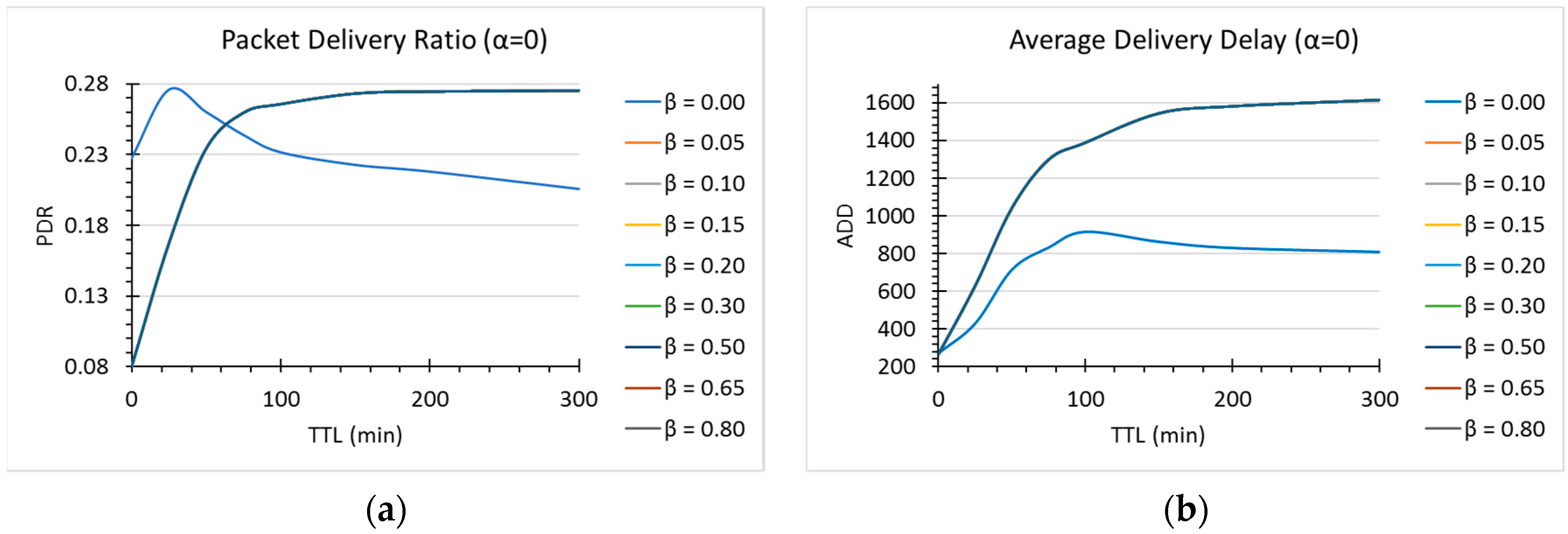
7.2. Effect of the Fitness Thresholds

As described in Section 5, the $\alpha$ parameter is a value that determines to what extent some of the connections are immediately discarded as next hop candidates. Intuitively, a very small value would mean that only a small portion of the current connections are discarded, so most of them have a chance to be chosen (although in descending order with respect to their fitness values). The limit is $\alpha =0$, and since $1\ge f\ge 0$, the condition $f\ge \alpha$ means in this case that all of the connections are considered as potential candidates. Similarly, a very large value of $\alpha$ will result in a strong limiting condition, meaning that only the very best hosts (the ones with considerably large fitness) will be considered as possible next hops. As we can infer from this explanation, the dynamics of the environment are strongly influenced by the $\alpha$ value. To better understand the effect of this fitness threshold, we run simulations changing this parameter with $\alpha =\left\{0, 0.05, 0.1, 0.15, 0.2, 0.3, 0.5, 0.65, 0.8, 0.95, 1.0\right\}$ and a msg TTL varying from $TTL=\left\{10,25,50,75,100,150,200,300\right\}$. A similar reasoning than that for $\alpha$ was made for the $\beta$ fitness threshold, so we considered $\beta =\left\{0, 0.05, 0.1, 0.15, 0.2, 0.3, 0.5, 0.65, 0.8, 0.95, 1.0\right\}$ in the simulations as well. We distinguished two main differentiators in both the $\alpha$ and $\beta$ values: $\alpha =0$ and $\alpha >0,$ and $\beta =0$ and $\beta >0$. In the first case, with $\alpha =0$, we can see that the cases $\beta =0$ and $\beta >0$ resulted in noticeable different dynamics (see Figure 5 and Figure 6). We notice that for $\alpha =0$, for TTL values smaller than 60, the performance of DLR+ is better with $\beta =0$ for PDR. For ADD, in turn, $\beta =0$ is the choice, as it showed better results than for other $\beta$ values.

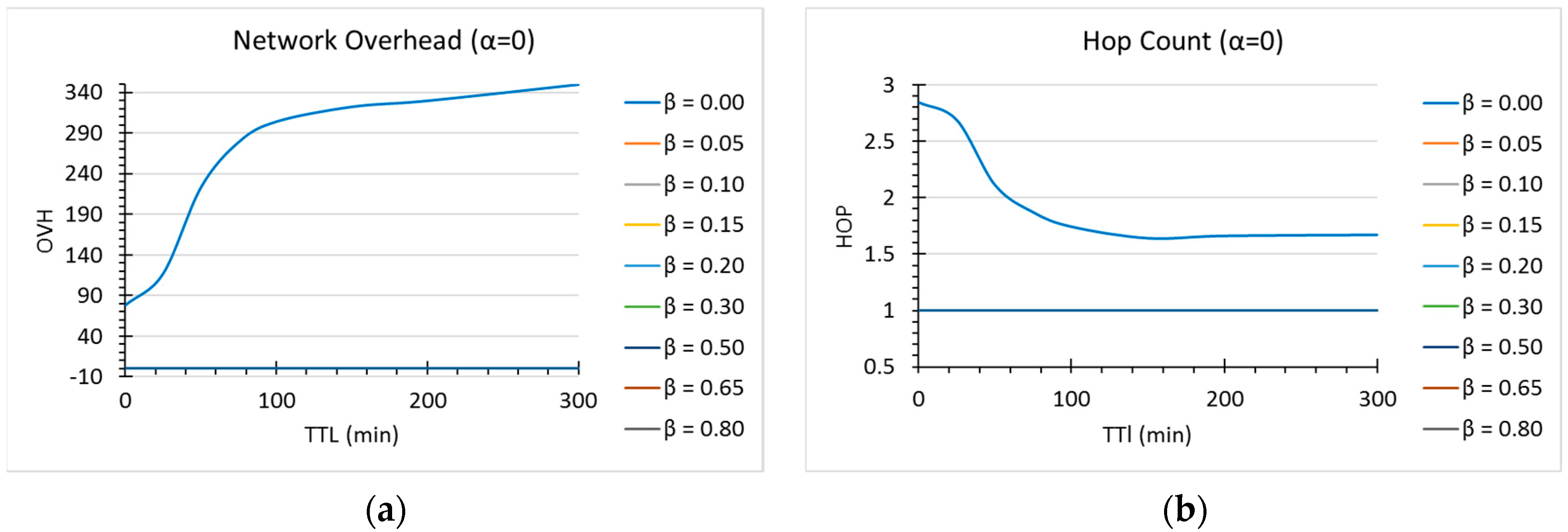
In any case, however, for OVH and HOP (Figure 6) the choice is any value different than 0 for $\beta$. As we can see, there is a tradeoff mainly between network overhead and delivery ratio or delivery delays, and the final choice of the parameters ultimately depends on the final application of the router in delay-tolerant networks (i.e., if we are interested in minimizing latency, at the expense of some overhead, or we have limited resources, such as in mobile sensor networks).

For $\alpha >0$, we did not notice any significant difference in the values of $\beta$. Finally, for $\alpha >0.5$ there was a slightly improvement in overhead and number of hops. For this version of DLR+, we decided to use $\alpha =0.65$ and $\beta =0$.

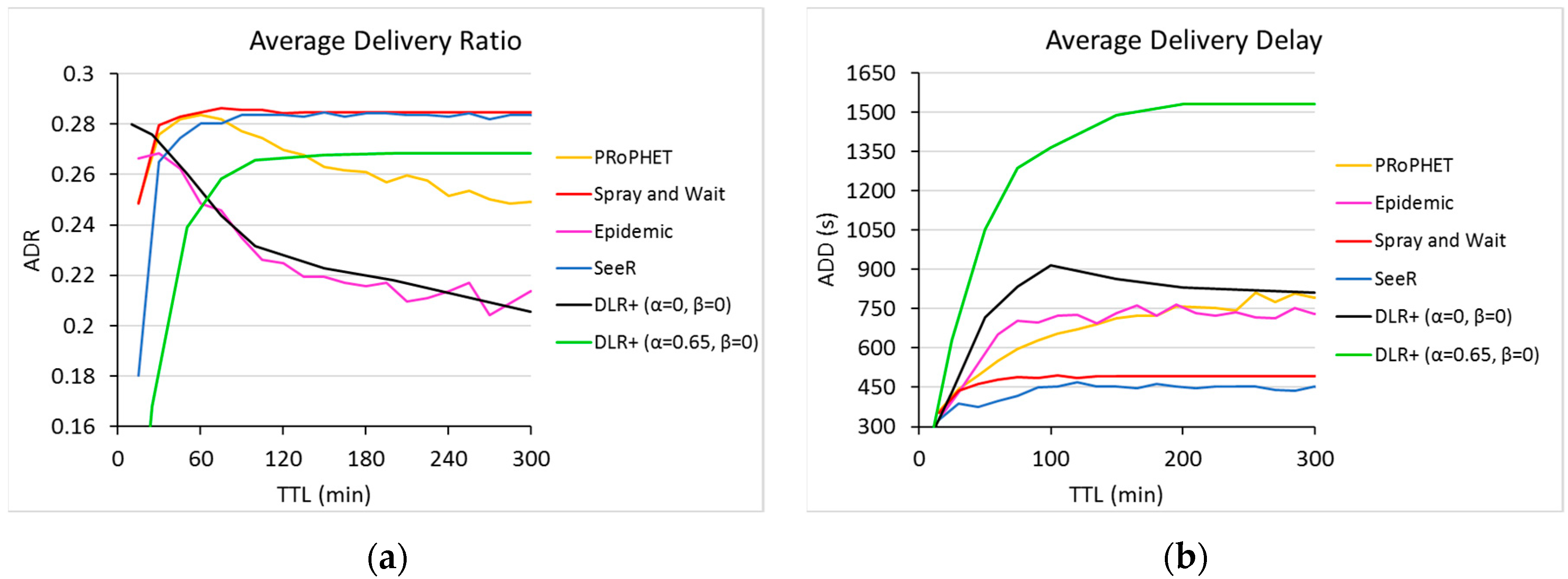
7.3. Performance of DLR+

In this subsection we discuss the final performance of DLR+ ($\alpha =0.65/0, \beta =0$) and compare it against other well-known routers (Figure 7 and Figure 8).

As can be seen in Figure 7a, DLR+ (α = 0.65) offers a greater PDR than the epidemic router and PRoPHET for TTL greater than 60 and 130, respectively. Although its performance on this metric is not the best, it is very close to those who offer the best values, only about 6.07% below its better counterparts. On the other hand, with α = 0, DLR+ outperforms all routers in PDR for TTL < 25. This reflects an interesting dynamic in the response of DLR+ for this case, in contrast with other routers: The more TTL is provided, the more inefficient the router becomes; however, as TTL is smaller, the response of the proposed router increases, outperforming the other routers in this metric. There is a tradeoff, nonetheless, in this range of operation, because in this part, DLR+ (α = 0) does not have the best performance in network overhead and hop count (Figure 8), although it shows acceptable values, very close to the ones generated by other routers.

As for delays, in the long run, DLR+ does not provide the best performance on average delivery delay (Figure 7b). We can see that as the TTL increases, so does the delivery delay values, and although they tend to stabilize at some point, there are significant differences with respect to other routers’ performance. The proposed router, however, performs fairly well for small TTL values, laying in points very close to those resulted from their counterparts, with roughly the same ADD values than those of other routers for TTL ≤ 25.

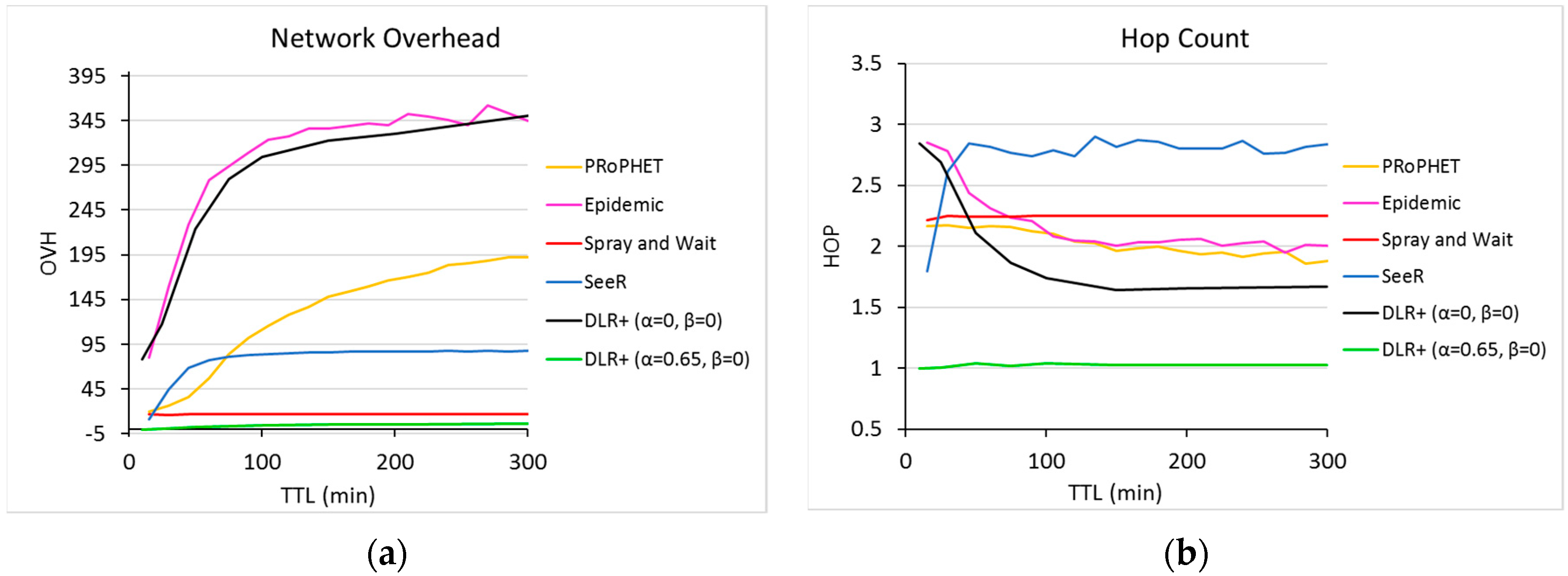
In network overhead (Figure 8a), DLR+ (α = 0) did not have the best results, with significant differences with respect to their counterparts, closely resembling the epidemic routing. For α = 0.65, however, DLR+ had the best performance, with nearly zero overhead, which means extremely efficient resource usage, way below the OVH values returned by other routers.

In hop count, on the other hand, with α = 0 the number of hops used by DLR+ is very close to a constant 1.6 in the long run, which shows better values than other routers. Indeed, for TTL > 50, the proposed router (α = 0) outperforms all other routers in the experiment, but even for TTL values smaller than 50, the number of hops used by DLR+ is between 2.2 and 2.8, which is a range in which all other routers lie as well. For α = 0.65, however, the proposed router shows an impressive HOP of nearly 1, which is a very significant difference with respect to the rest, confirming the highly efficient usage of network resources.

8. Conclusions and Future Work

The integration of vehicular networks in intelligent transportation systems will bring a vast set of new services in areas such as traffic management, security and safety, e-commerce, and entertainment, resulting in a global evolution of cities as we know them. The deployment of this kind of network, however, is slowed down by the intrinsic severe conditions of its environment. Among others, routing in vehicular delay-tolerant networks is a research challenge that requires special attention, since their efficiency will ultimately dictate when these networks become real life implementations. In this paper, we have modeled a solution to the routing problem in VDTN and presented a router based on deep learning, which uses an algorithm that leverages the power of neural networks to learn from local and global information to make smart forwarding decisions on the best next hop and best next message. As discussed in the previous section, the proposed router presents improvements in network overhead and hop count over some popular routers, while maintaining an acceptable delivery rate and delivery delay. For TTL ≤ 25, if resources are not a problem, it is recommended to use DLR+ with α = β = 0, as it will provide the highest delivery ratio. On the contrary, if network resources are a concern, the proposed router is recommended to use with α = 65 and set the message scheduler to β = 0, so it has the highest performance despite the resource limitation.

In the future, the DLR+ router can be further developed, including the full integration of the neural network to work in real time and automatic online parameter tuning to increase the overall performance. Also, more features of the host and messages can be added to the paradigm, so the router gets an even better understanding of its environment.

As discussed earlier, there has to be a trade-off between some of the metrics that are sought to be optimized to achieve an overall better performance in the VDTN, and the quest for this continues. Ultimately, the corresponding trade-offs depend on the particular application of the network; for instance, in mobile sensor networks, the delays may not be an important thing, but the limited resources might be, whereas in VDTN, there can be a certain level of flexibility depending on even more specific applications, such as e-commerce transactions versus entertainment applications. All in all, the DLR+ router provides an insight into how deep neural networks can be used to make smarter routers, and this work provides a framework than can serve as a starting point to build more intelligent routing algorithms.