Improved Current Estimates from Spar Buoy-Mounted ADCP Measurement Station: A Case Study in the Ligurian Sea

Abstract

Current measurements in the open sea are generally acquired by Acoustic Doppler Current Profilers (ADCPs). In the case of ADCPs mounted on spar buoy, current profiles require to be post-processed, to properly take into account the buoy influence: in fact, ADCP compass may reflect alterations induced by the metal structure of the buoy and apparent currents can occur due to the large displacement of the platform. Uncertainty analysis is finally required to properly consider both these effects and to compute robust velocity estimates. A new methodology is tested for a measurement station in the Ligurian Sea, where an ADCP was mounted on the surface buoy of the W1-M3A (Western 1 Mediterranean Moored Multisensor Array) oceanographic observatory, facing upwards at the depth of about 40 m. Marine current numerical models and historical data in the area have been used as a basis for comparison to test the consistency of the proposed method. A very good agreement is obtained. Only minor discrepancies are reported (e.g., monthly averages from the reference model slightly underestimate the west-east current component along the entire profile), but, in general, the application of the proposed methodology ensures that the spar buoy-mounted ADCP system is able to provide reliable measurements for oceanographic studies and validation of 3D hydrodynamic models.

1. Introduction

Current data are a major asset for oceanographic research both for validation and assimilation in hydrodynamic models. Current monitoring is also an essential tool for understanding ocean marine ecosystems, planning and securing maritime operations or designing offshore structures. The measurement of current is the basis for any resource assessment related to offshore renewable energy devices. Accurate current data can help in tracking sources of pollution, like chemical or sewage spills. Same data can be used to efficiently and reliably forecast oil spill trajectories or assess coastal water quality in general. Reliable information on current conditions and consequent monitoring are also required for habitat restoration or coastal protection projects, especially considering the future spread of nature-based solutions (NBS).

Many efforts have been made in the last decades to monitor ocean currents using Lagrangian and Eulerian platforms. Classical Lagrangian platforms (i.e., drifters and floats) could infer current measurements over a wide area only through indirect methods, although Argo floats have been recently upgraded to host high frequency acoustic current meters. Modern autonomous moving platforms (i.e., gliders and other types of marine drones) can further increase spatial and temporal sampling of ocean current since most of them can submerge for long periods to get measurements at a particular depth, but cannot provide long term time-series at fixed point. High frequency coastal radar can ensure continuous monitoring of surface ocean currents at proper spatial and time scale (range up to 200 km and time intervals typically of 1 h), but cannot provide information about the current profile along the water column. Eulerian platforms (i.e., buoys and moorings) may collect in-situ current observations at a high temporal resolution along the water column, if their scientific payload includes array of current meters or Acoustic Doppler Current Profilers (ADCPs).

The issue of temporal and depth coverage is commonly tackled by ADCPs. They are based on the principle of Doppler Shift: they emit an acoustic signal and receive it backscattered by the particles moving at various depths in the water column due to current action [1]. The profile of speed and direction of the current at different depths is then calculated from the frequency shift of the backscattered signal. ADCPs are normally deployed on the seafloor, fixed along mooring lines, or mounted inside the keel of a boat (vessel-mounted), but can also be mounted on spar buoy. In that case, current profiles require to be post-processed to properly model the buoy influence. The following two effects occur, both attributable to the buoy action on the ADCP:

• alterations of the ADCP compass due to the local distortion of the Earth’s magnetic field induced by the metal structure of the buoy: such distortion is not constant over time due to the rotation of the buoy itself caused by winds, waves and currents;
• apparent currents measured by ADCP due to displacements of the buoy following the action of currents and winds: in case of long mooring line, the buoy is in fact free to move around the anchor.

An ad hoc uncertainty analysis is then required to properly consider both these effects and to compute robust velocity estimates. As regards metal body interference, Munchow et al. [2] tested a submerged towed vehicle with both an upward- and a downward-facing ADCP, designed to have a minor exposure to surface disturbance and wave wake. They stressed for the first time the need for a careful in-situ calibration of magnetic compass, to remove the magnetic variation induced by the ship’s hull and the tow platform and to improve the accuracy of the data. The correction of errors on direction measurements brought by the current profilers installed on mooring cages is introduced by Le Menn et al. [3], who developed a calibration platform for magnetic compasses and tilt sensors, following a method perfected in 2007. In combination with this platform, [4] suggested an approach based on the measurement of the frequency of pulses and on the simulation of received echoes, allowing the logging and calibration of most of the current meters manufactured by Nortek Instruments.

The main focus of the present work is illustrating the details of an experimental activity aimed at measuring current profiles in open sea using an ADCP mounted on a spar buoy: the proposed methodology, from the set-up of the experiment to its implementation, from recovery to data post-processing is described in the following.

The paper is organized as follows: a brief description of both the W1-M3A (Western 1 Mediterranean Moored Multisensor Array) oceanographic infrastructure and of the used ADCP is illustrated in Section 2. In Section 3, the sea-current dataset is analyzed as an applicative case study of the post-processing correction methodology, that is discussed in detail: actually, the application of the method must be understood as a result, rather than the interpretation of the data from an oceanographic point of view. Discussion is covered by Section 4, where comparisons with historical data and numerical models in the area are presented to test the consistency of the proposed method, together with its uncertainty analysis performed as an example on a sub-set of data. Conclusions, together with directions of future work, are drawn in Section 5. The collected dataset, together with the proposed post-processing techniques, allowed to achieve a basic knowledge, aimed at implementing a monitoring system able to operate reliable ADCP measurements even from this kind of moving platforms, or from profiling floats equipped with ADCPs ([5]).

2. Experimental Setting: The W1-M3A Spar Buoy and the ADCP

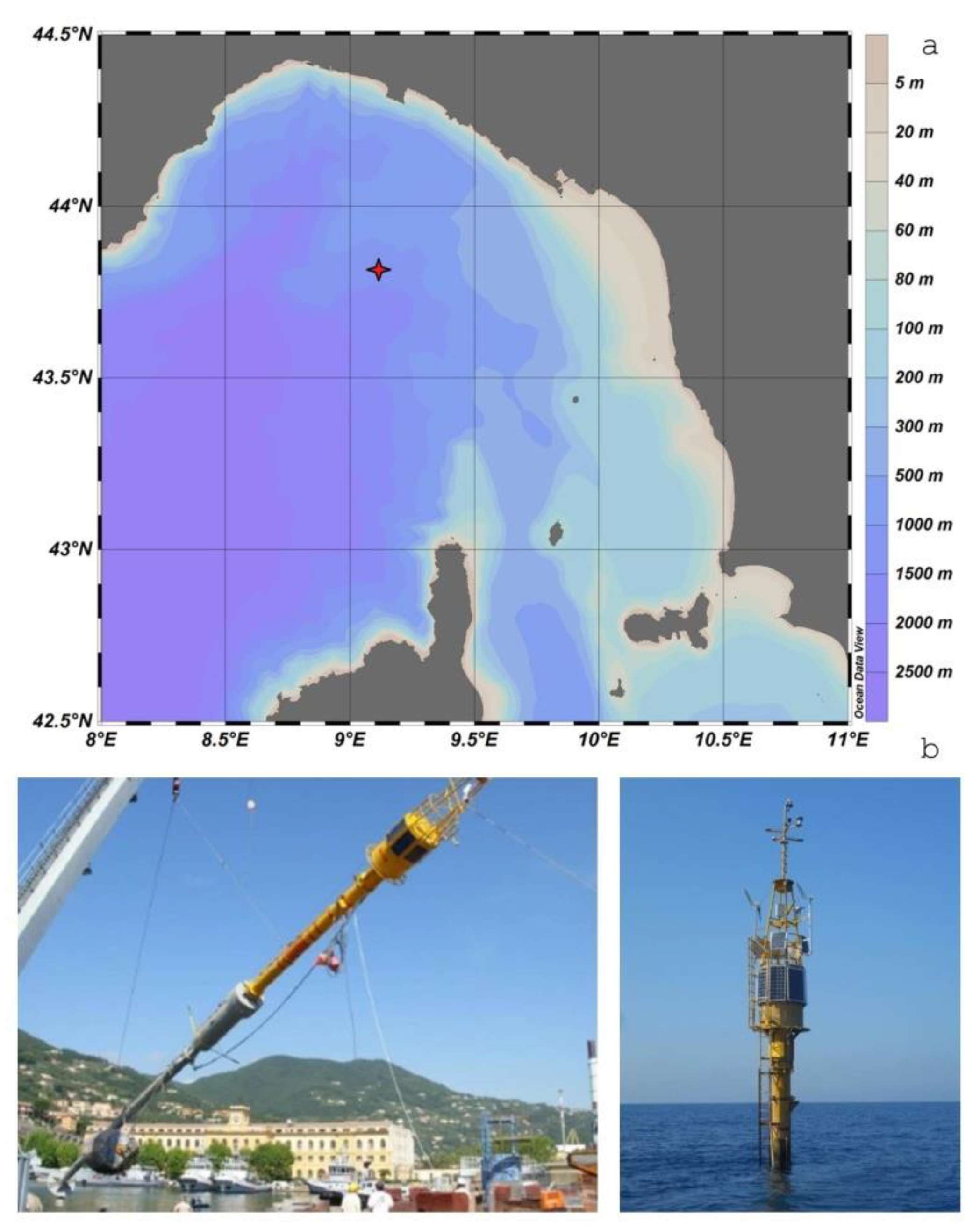
The W1-M3A is located about 40 NM offshore Genoa, on a 1270 m deep sea bed [6,7] (43°48.90′ N, 09°06.80′ E) (Figure 1a). The observatory is composed of two sub-systems, a large spar buoy (known as “ODAS Italia 1”, 51 m long of which about 37 m immersed and 12 tons weight, shown in Figure 1b: ODAS, or more simply buoy, in the following) and a sub-surface mooring acquiring oceanographic data down to the ocean interior. The Buoy is a completely autonomous laboratory that is part of the of European Multidisciplinary Seafloor and water-column Observatory and of the Integrated Carbon Observation System-European Research Infrastructure Consortiums (the EMSO and ICOS-ERIC respectively). Its power supply is guaranteed using solar and wind energy, while the communication is ensured through satellite connection. Monitoring the meteorological conditions of the basin and the physical and biogeochemical status of the area, the Buoy is a useful support for operational oceanography and for meteorology centers, contributing to weather and marine modeling and forecasting, and allowing us to develop comparisons between the observations from satellites and in situ measurements.

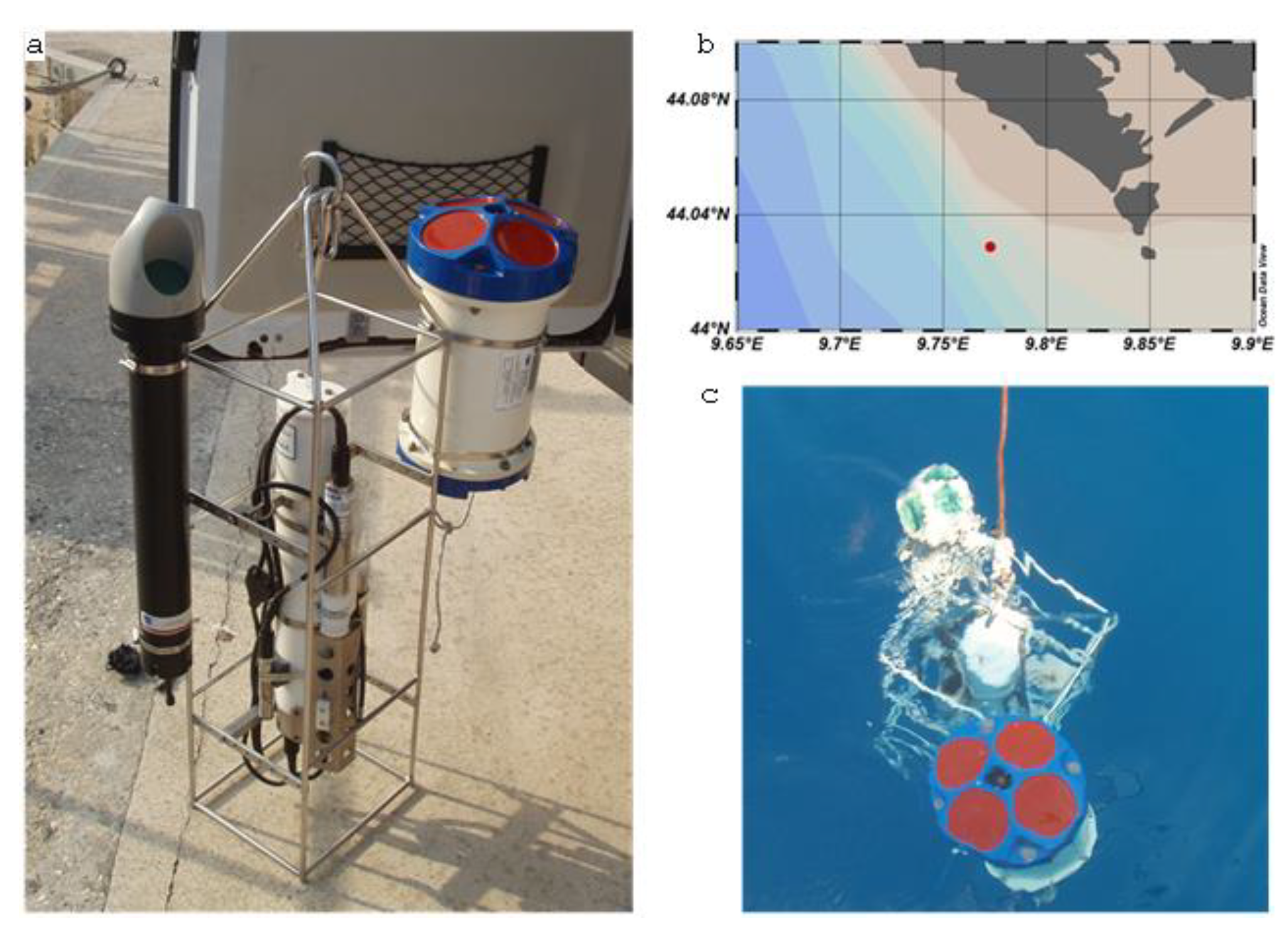
A three-beam ADCP, manufactured by Nortek (model Aquapro, [8]), was selected in order to avoid the possible interference of a fourth beam with the structure of the Buoy. The general characteristics of the instrument are reported hereafter:

• acoustic frequency: 400 kHz;
• max working depth: 200 m;
• max profiling range: 60–90 m;
• cell size: 2–8 m;
• beam width: 3.7°;
• min blanking distance: 1 m;
• max number of cells: 128;
• velocity range: ±10 m s⁻¹;
• accuracy declared by the manufacturer: 1% of measured values ±0.005 m s⁻¹;
• max sampling rate: 1 Hz.

Before the installation on the buoy, the Nortek ADCP was verified against a four-beam RDI ADCP (Figure 2), at water depth of about 37 m, comparable with the damping disk depth of the Buoy. Same general settings and the ENU reference system (East-North-Up coordinates) were configured for both the ADCPs, with automatic correction of roll, pitch and heading. The two ADCPs were installed on the frame of a CTD probe, with reference beams facing the same direction (beam X for the Nortek, beam no. 3 for the RDI). Mean current measures of the two ADCPs, along the water column, resulted reasonably comparable inside their standard uncertainties, calculated as the standard deviation of the collected datasets (e.g., at the depth of 18 m, Nortek and RDI measured a mean north component of the current equal to (6.7 ± 1.5) cm s⁻¹ and (5.6 ± 1.7) cm s⁻¹, respectively).

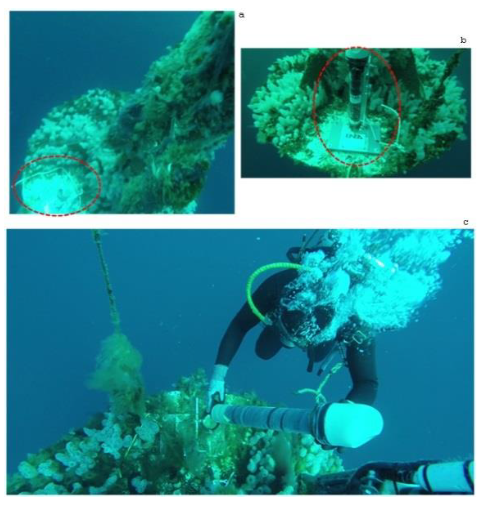
The ADCP was then set to collect current signals at 1800 s intervals (average measure as a result of 900 s acquisition period, with 10 s compass update rate), in ten 4 m-long depth cells, with a (nominal) horizontal velocity precision of 0.006 m s⁻¹. The ADCP mechanical configuration on the Buoy was properly designed to avoid any interferences of the acoustic beams with the Buoy structure: ADCP was placed on the damping disk of the Buoy at the depth of about 37 m and facing upwards (Figure 3). Specifically, the frame of the ADCP was clamped by divers to pre-existing bolts that were fixed to the damping disk when the buoy was in the dry dock. By this way, it was assured that any frame attached to those bolts was perfectly aligned to the bow of the buoy. Current measures were continuously collected for a period of 5 months (from April to August 2017, with a brief interruption due to battery change, for a total of 7256 current profiles).

3. Results

In the following, post-processing of ADCP data is described, step-by-step.

3.1. Estimated Average Depth of the ADCP during the Deployment Period

From the pressure measurements recorded on board of the ADCP, the average depth of the head of the acoustic sensor was derived, in order to correctly scale the depths associated with the centers of the various cells into which the current profile was divided. The procedure can be described in the following points:

• average deployment pressure of the ADCP throughout the entire deployment period (and associated standard deviation):

$${\overline{p}}_{ADCP}=\left(37.46\pm 0.20\right) \mathrm{dbar}$$

• conversion of pressure in depth, taking into account the following parameters:

  -

  average position of the buoy, in terms of latitude: 43.8430° N,

  -

  average temperature measured by the ADCP: 15.98 °C,

  -

  average salinity (from historical data, a priori set in the ADCP configuration): 38,

the average depth to which the ADCP was deployed is the following:

$${\overline{d}}_{ADCP}=\left(37.16\pm 0.20\right) \mathrm{m}$$

• from the calibration certificate provided by Nortek, the pressure measurements on board the ADCP were declared with a tolerance of ±0.5% of the full scale (200 m). The contributions due to drift over time, resolution and uncertainty associated with the single pressure measurement were compassed in this range of variability. By combining the various contributions of standard uncertainty, the following measurement of the average depth of immersion of the ADCP was finally obtained:

$${\overline{d}}_{ADCP}=\left(37.2\pm 0.6\right) \mathrm{m}$$

• the valid measuring range of the ADCP could be estimated from the well-known empirical formula [8] (where θ = 25° indicates the angle of the single beam with respect to the vertical):

$$\Delta L_{ADCP}={\overline{d}}_{ADCP}\times \cos \theta -cell size ~ 30 \mathrm{m}$$

The measurement range is therefore valid for depths between about 37 m and 7 m: considering that there is 1 m of blank, cell num. 8, whose center is located about 4 m deep, is the first of the critical cells in terms of accuracy (and will therefore be excluded from the analysis).

In conclusion, the actual depths of the cells constituting the current profiles measured by the ADCP are shown in

Table 1. Actual depths at which the centers of the ADCP measurement cells are located: depths for which the current measurements were not considered valid are shown in gray background. Negative depth indicates the cell whose center is in the air, above the surface of the sea.

Cell No.	Cell Center Distance from Sensor Head	Cell Center Depth
	m	m
1	5	32.2
2	9	28.2
3	13	24.2
4	17	20.2
5	21	16.2
6	25	12.2
7	29	8.2
8	33	4.2
9	37	0.2
10	41	−3.8

.

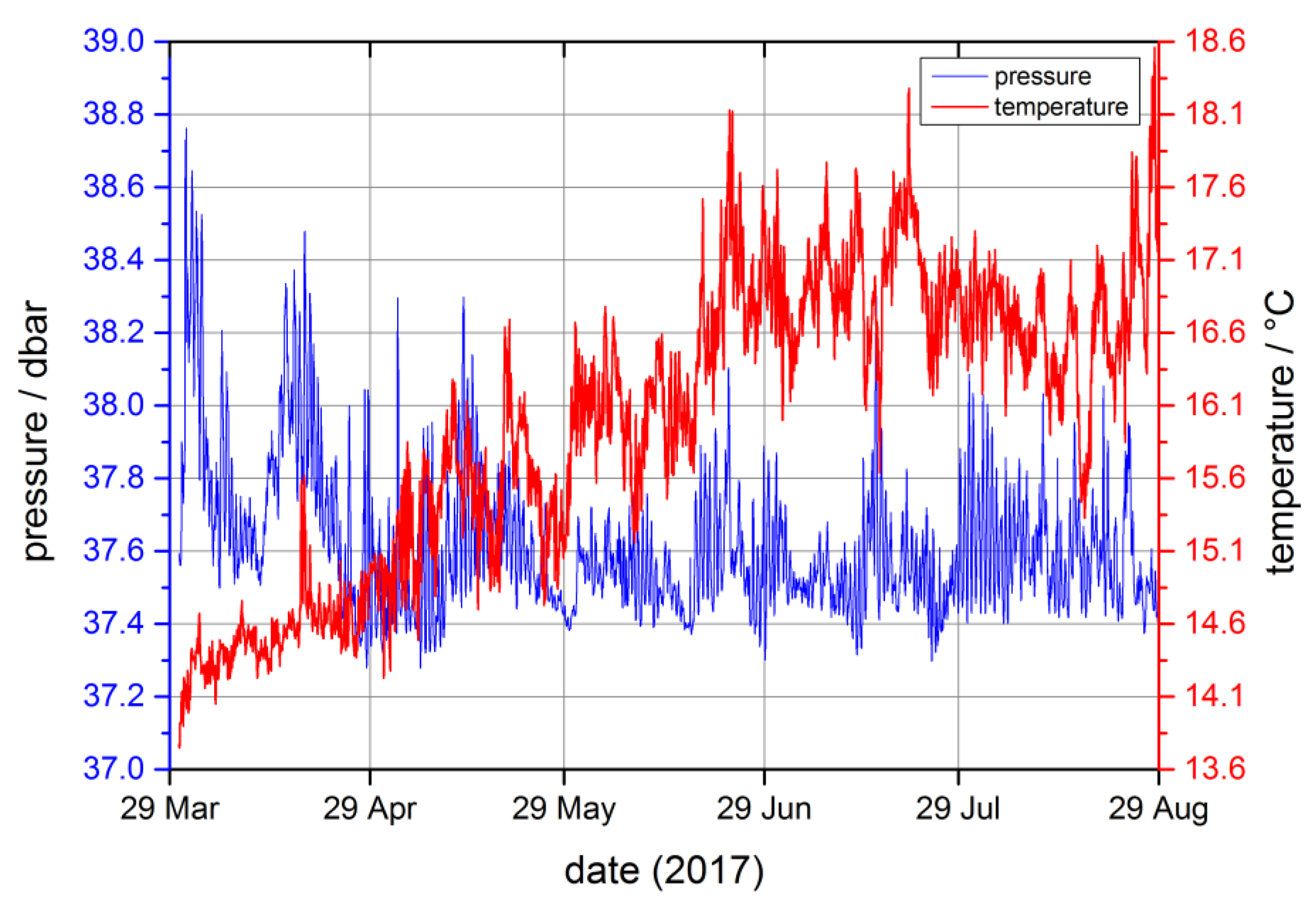
As additional information, Figure 4 shows the trends over time of the pressure (and temperature) values recorded by the sensors on board the ADCP: pressure oscillations, thanks to the damping action of the Buoy disk, are always much lower than the bin size of 4 m.

3.2. Intensity Check on the Three Acoustic Beams of ADCP

To verify that the acoustic signals recorded by ADCP show no anomalies, the average values (vs time) of the counts on the three acoustic beams were compared, for each cell depth (Figure 5a).

It can be noticed how the three beams behaved in a homogeneous manner (within the respective standard deviations): in fact, acoustic signals correctly decreased towards the sea surface (due to an increase of the distance from the emitting/receiving sensor). Greater consistency was found for the cells in the range 2 to 7. For what concerns cells no. 10, 9 and 8 their exclusion from the analysis of the current profiles was confirmed: positions of cells no 10 and 9 were directly in air and close to the water–air interface, respectively. Cell no. 8 was characterized by an excessively high number of counts (if compared to deeper cells): this may be due again to the water–air interface effect.

Finally, the signal-to-noise ratio (SNR) of the echo signal was maintained at acceptable levels during the whole measurement period, for all the three acoustic beams (Figure 5b).

3.3. Buoy Heading and GPS Data Matched with ADCP Data: Correction for Heading Error and for the Velocity Vector Associated with the Buoy Displacement

In accordance with procedure described in detail in [9], to ensure the correct matching between ADCP and buoy data (acquired at half an hour and every hour, respectively) it is necessary to interleave the data of the latter, in terms of its heading and GPS longitude–latitude values. Velocity vector (in terms of modulus and bearing) associated with buoy displacement can then be calculated by applying the well-known spherical law of cosines formula [9,10].

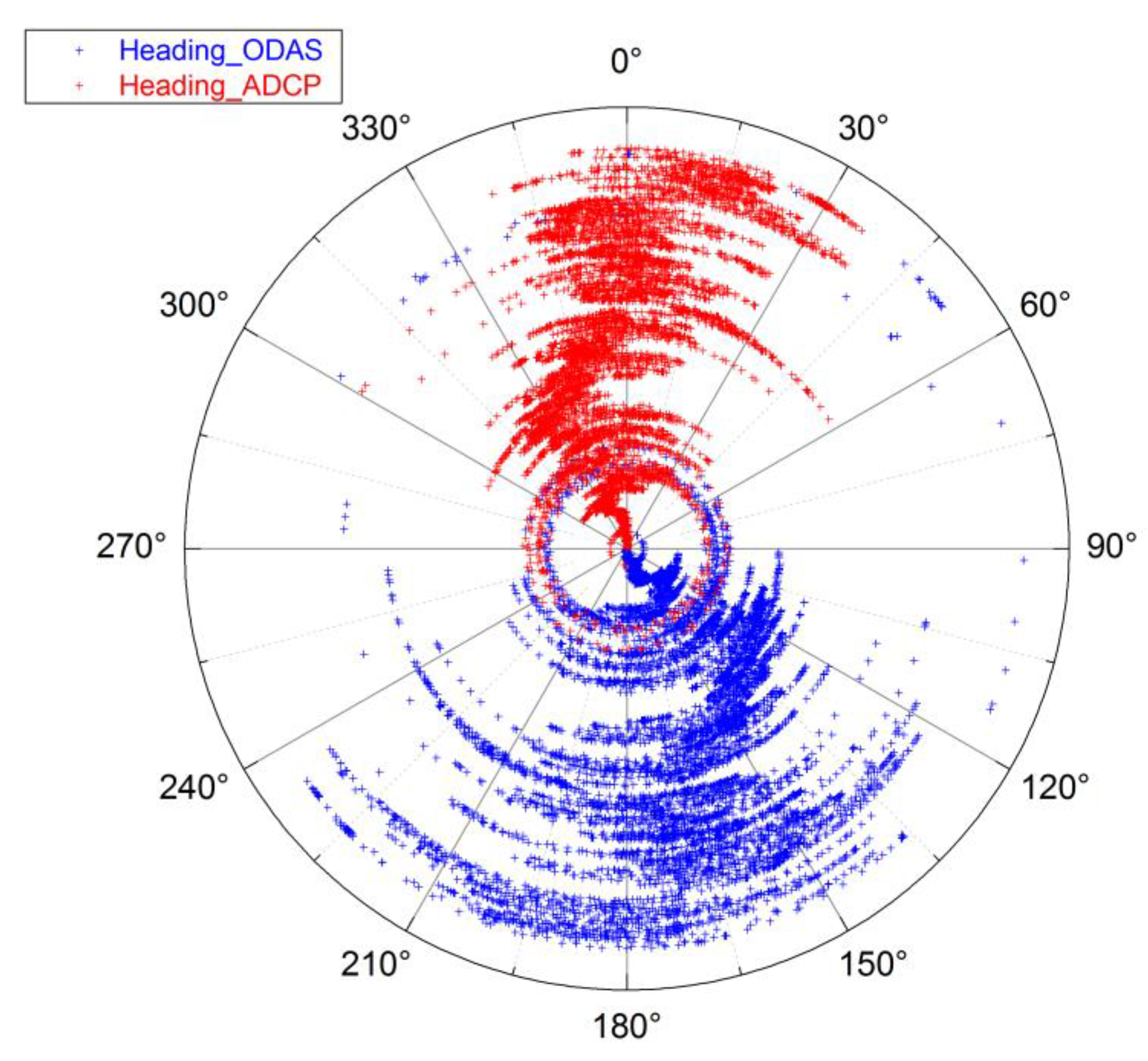
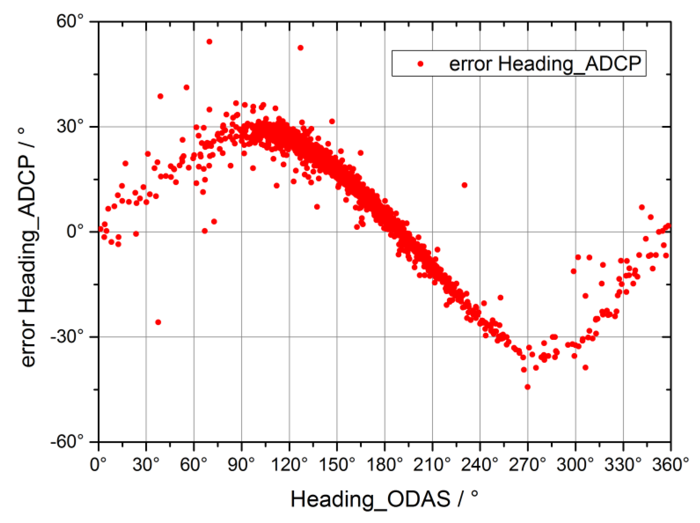
First of all, since ADCP compass values could be potentially influenced by the presence of the metal body of the buoy, the ODAS heading measures were adopted as a reference and consequently the correction to be adopted on the ADCP measures is evaluated. The heading values for both the ODAS and the ADCP are shown in Figure 6 (where the value of 0° indicates the north direction, as per convention).

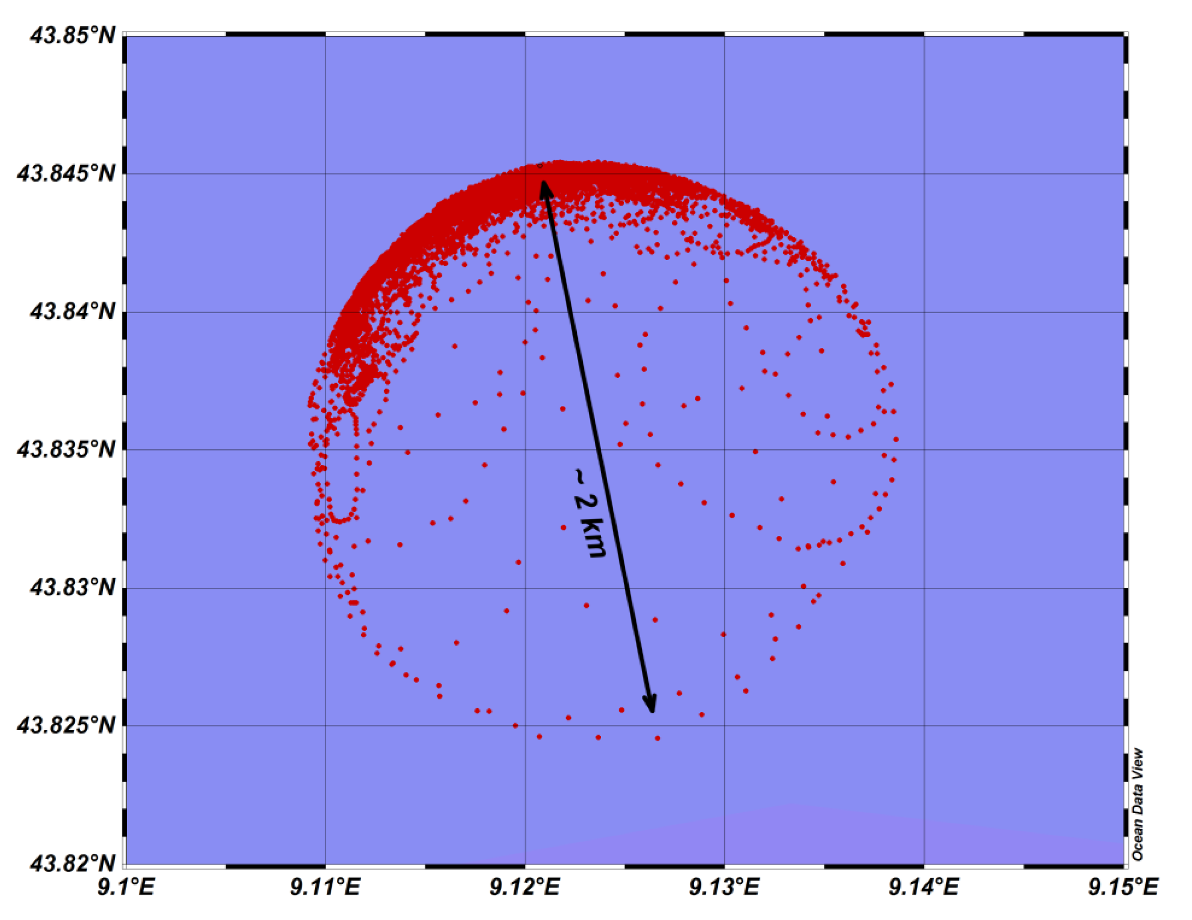
The analogy with the information obtainable from the GPS position of the buoy (Figure 7) can be noticed: the buoy, in fact, remained usually in a stationary position for most of the time in a direction approximately equal to the North-North-West, evidently put in traction by a current and/or by the action of winds coming from South-South-East. Being the mooring attachment point the mechanical reference of the buoy used to define its orientation (or heading), it can be noticed that the buoy heading values were those expected, that is, on average positioned in the 2nd quadrant (South-South-East, Figure 6).

At the same time, since the ADCP was mounted at the antipodes with respect to the buoy mooring, it can be observed that the ADCP heading values were reversed compared to those of the buoy, unless an error was to be evaluated and then corrected for each ADCP data acquired.

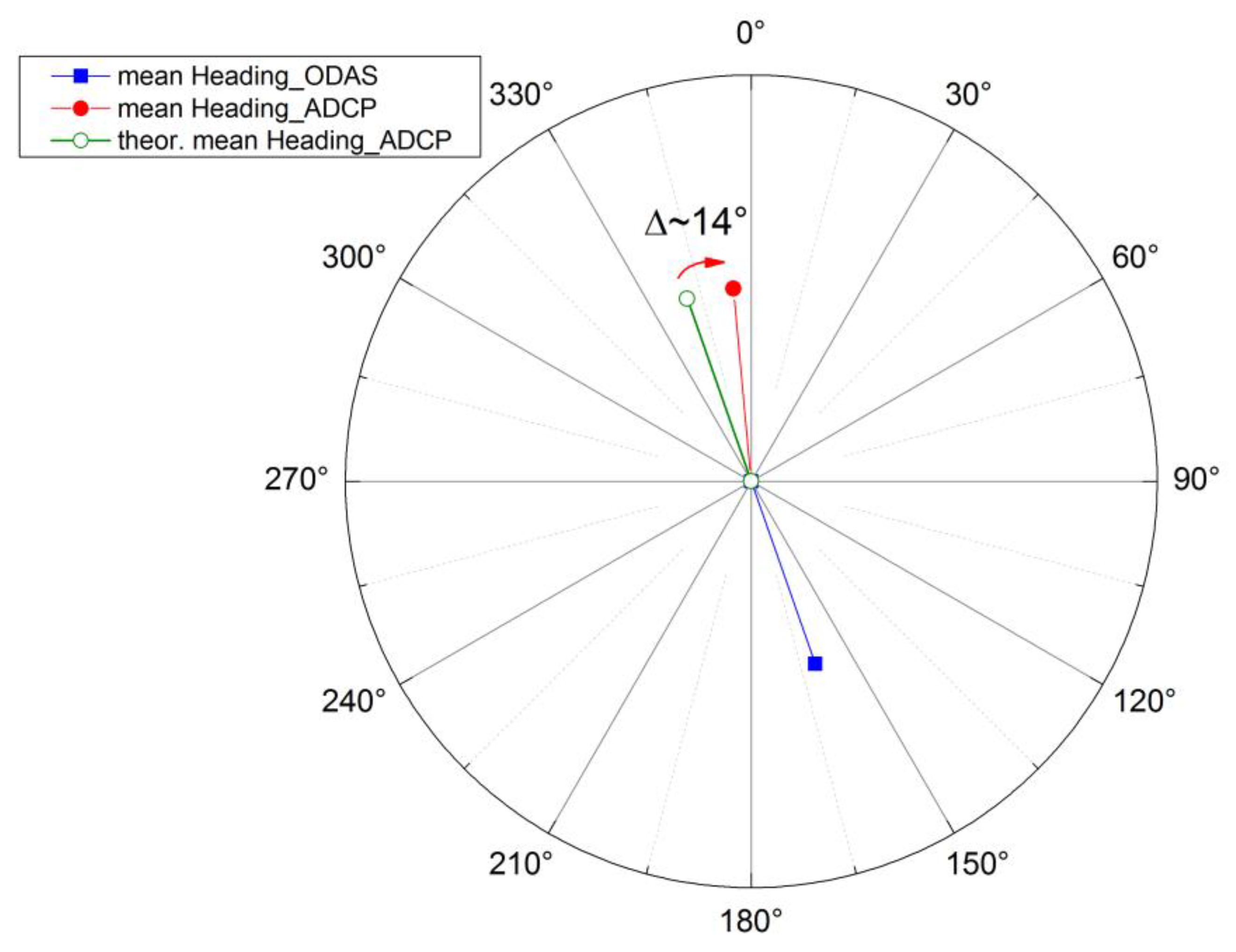
A mean evaluation of ADCP heading error can be obtained as follows: averaging the values shown in Figure 6, the average heading measured for the buoy and ADCP, respectively, is obtained in the same period. From the first of the two values, adding an angle of 180°, the theoretical average direction of the ADCP heading is then obtained. It can be seen (Figure 8) how this value differs from the average value measured by the buoy by about 14°: it can be concluded that this is on average the value of the phase shift induced by the metal body of the buoy on the compass of the ADCP.

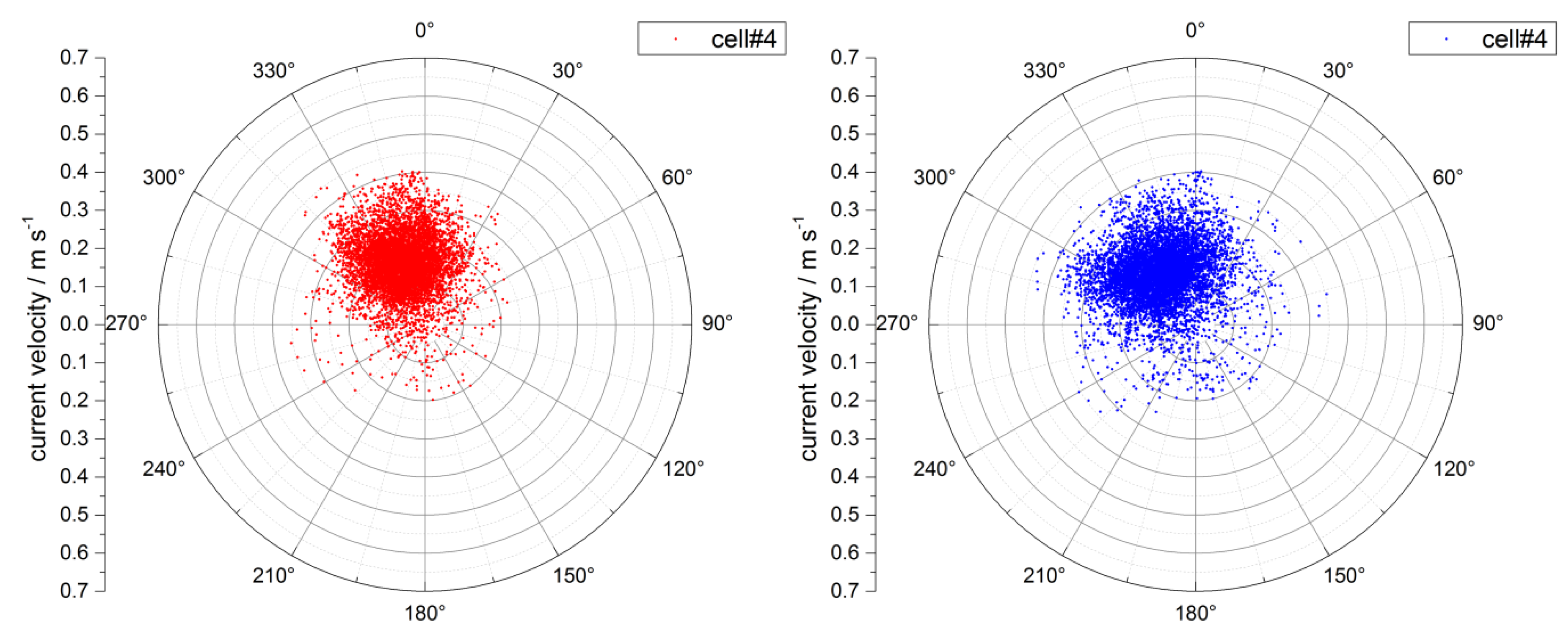
Actually, the correction of the ADCP heading by means of buoy heading was carried out for each individual profile acquired: the difference between the two values (which is an estimate of the error made by the ADCP compass for the measurements taken every half hour) was subtracted from the various angles of the current velocity vectors cell by cell, profile by profile. As an example, Figure 9 shows the effect of the heading correction for the current measurements detected at cell no. 4 (in the middle of the useful profile, at a depth of about 20 m).

Finally, Figure 10 shows the overall trend of the ADCP compass error as a function of the buoy compass values, showing how this effect depended on the orientation of the buoy itself.

After the correction for heading error, ADCP data were ready to be corrected for the relative buoy movement. Since the buoy, in addition to rotation on its own axis, moved in the plane under the action of current, waves and/or winds, the ADCP was affected by apparent currents for which the measured current profiles had to be corrected. If the buoy moved with velocity v, the ADCP measured an equal and opposite apparent current -v: the correction for the ODAS movement could then be implemented by vectorially composing the buoy and ADCP velocity vectors cell by cell, profile by profile.

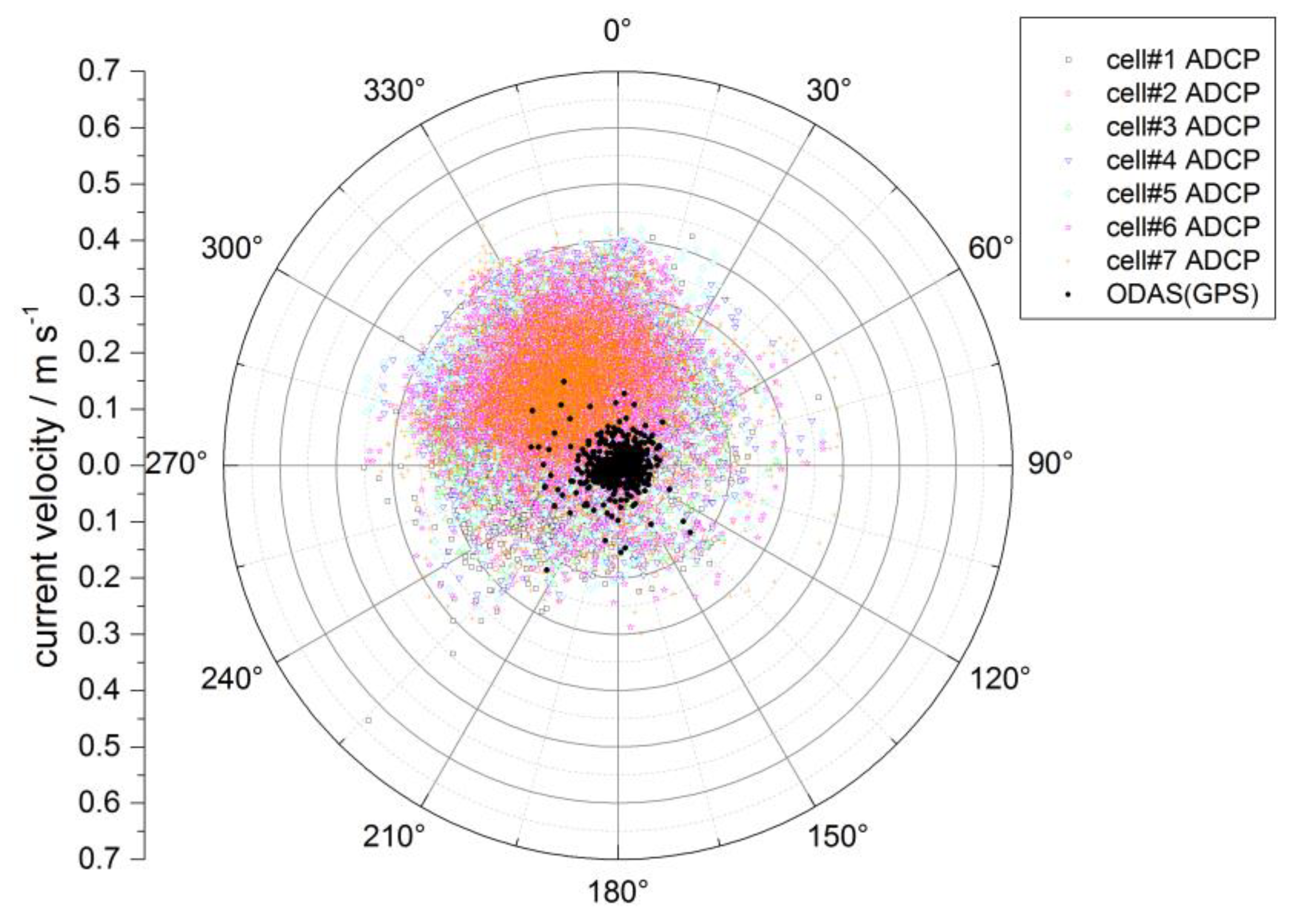
Figure 11 shows in polar coordinates an overview of all the velocity vectors measured by the ADCP in the seven considered cells (already corrected for the buoy heading), together with the velocity vectors of the buoy derived from GPS measurements.

Finally, Figure 12 shows the polar diagrams relating to all corrected currents values in the two cells at the extremes of the profile range (cells 1 and 7, at depths of about 32 m and 8 m, respectively), during the period considered: these were the final values of the current profiles, corrected both for the buoy heading and for the displacement of the buoy itself. The information contained in Figure 12 is part of final, corrected experimental dataset: it had to be intended as the best estimate provided by the implemented method.

4. Discussion

Based on the methodological approach described in Section 3, an overall assessment of data-set consistency is hereafter discussed. To evaluate the results of the applied corrections, an analysis of the obtained currents temporal evolution and general characteristics was performed. In the lack of other independent and concurrent ADCP measurements, as well as of a reliable climatology to assess the consistency of the data set, a comparison was done with available ADCP measurements collected in the area during the past years, and with results from numerical model.

General characteristic of the observed currents are resumed by the progressive vector (Figure 13) and basic statistics. Currents in the surface layer are directed to the North-West at an average speed of about 19 cm s⁻¹ over the whole period of measurements, in accordance with the general circulation scheme of the Ligurian Sea [11,12] and previous ADCP observations from the same area [13]. Vertical structure is quite barotropic: currents have almost the same pattern at each level, with some attenuation of the speed with the depth.

Complex correlation coefficients are lower than expected (0.6–0.9), considering the high vertical resolution (each cell is 4 m) of the measurements and the short water column examined, probably resulting from a few cases having more than 15 cm s⁻¹ difference in magnitude of single measurements between two adjacent cells.

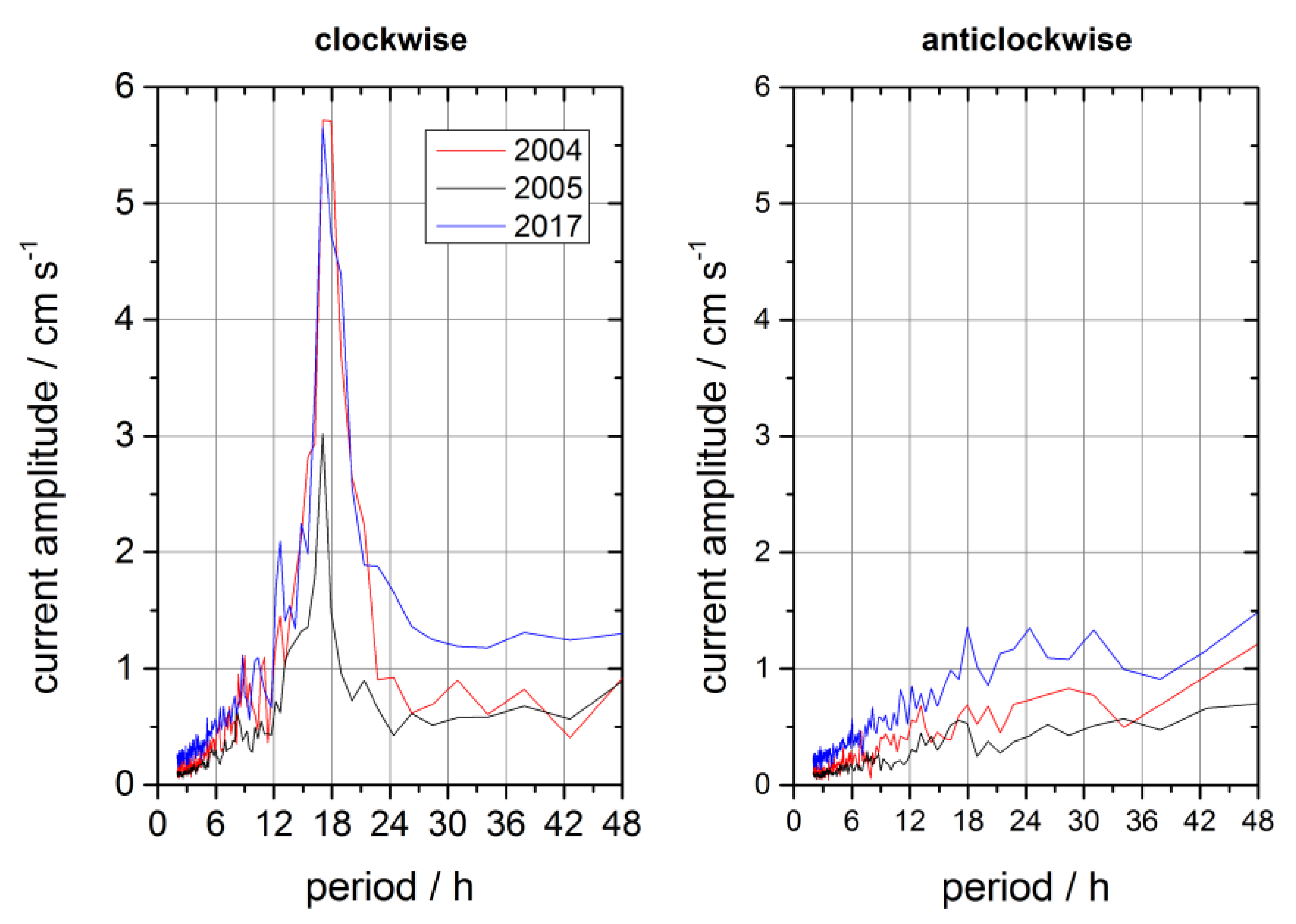
Rotary spectral analysis was performed by means of FFT on 11 subsamples 340 h long, that were then averaged. The clockwise spectrum is dominated by the inertial period, which is 17.3 h at this latitude; a small relative maximum appears on 12 h period only in the clockwise part, while in the anticlockwise part there are no relevant signals, apart from a small peak at about 17 h. Inertial rotations are also well evident in the progressive vectors at all depths; this is well consistent with the Ligurian Sea circulation, where inertial movements account for the great part of sub-daily variability [14].

Existing ADCP data-set collected in the area during the same season [13,15], were recovered and re-analyzed. Period of measurements and setting are resumed in

Table 2. Period of measurements and settings of the ADCP measurements used for the comparison.

Periods of Measurements	ADCP Depth	dz	dt
(a) 30/3–24/5 2004	62 m	8m	1 h
(b) 30/3–16/4 2005	100 m	8 m	1 h
(c) 19/4–29/8 2005	80 m	8 m	30 min

. The ADCP was a 300 kHz RDI looking up, located on a fixed mooring deployed close to the buoy (43°47.77’ N; 9°02.85’ E). As the depth of the ADCP changed from one deployment to the others, only the time series of currents collected at the bin including the layer at 22–24 m depth, which is a common depth for all the samples, were selected for the comparison.

The two time series of 2005 were merged after hourly averaging the time series sampled at 30 min. The resulting time series (bc) covers the correspondent period of the 2017, apart from 38 h of missing data which were replaced by a constant value in order to preserve the temporal evolution. Basic statistics are reported in

Table 3. Temporal averaged magnitude with standard deviation and direction of currents at the cell including 22–24 m depth. Letter a stands for current measurements collected in 2004, while bc indicates the two time series merged for year 2005. O indicates the ADCP measurements from the spar buoy.

22–24 m	a	bc	O
Magnitude cm s−1	13.9	6.8	17.7
Magnitude std cm s−1	7.0	4.7	6.4
Direction °N	330	280	294

.

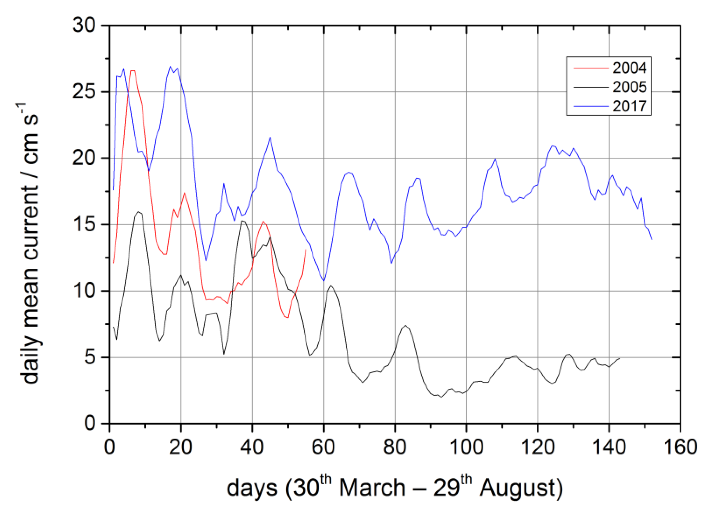
Despite 2017 summer currents are higher in respect to 2005, the comparison of the temporal evolution of daily mean currents (Figure 14) reveals relevant common features. In particular, an important mesoscale variability, which characterizes the early spring and summer circulation of the area [11,16], is found in all the three examined samples. A comparison with rotary spectral analysis on both a and bc samples (Figure 15) confirms the dominance of this variability and shows quite the same amplitude of that of 2004.

After the comparison with historical in-situ measurements in the area, experimental data have been compared with available results from numerical simulation in the area, to further evaluate the reliability of the corrections applied by the post-processing method. The E.U. Mediterranean Copernicus Marine Environmental Monitoring Service (CMEMS, http://marine.copernicus.eu, accessed on the 1 March 2021 ) physical system has been selected [17], and in particular monthly current data mean from the Mediterranean physical reanalysis product [18]. It is composed of a hydrodynamic model, supplied by the Nucleous for European Modelling of the Ocean (NEMO), and of a variational data assimilation scheme (OceanVAR) for temperature and salinity vertical profiles and satellite Sea Level Anomaly along track data. The horizontal resolution is approximately 5 km and there are 141 unevenly spaced vertical levels. The grid-model closest to the position of the buoy has been identified, corresponding to a distance of about 3 km from the average position of the buoy.

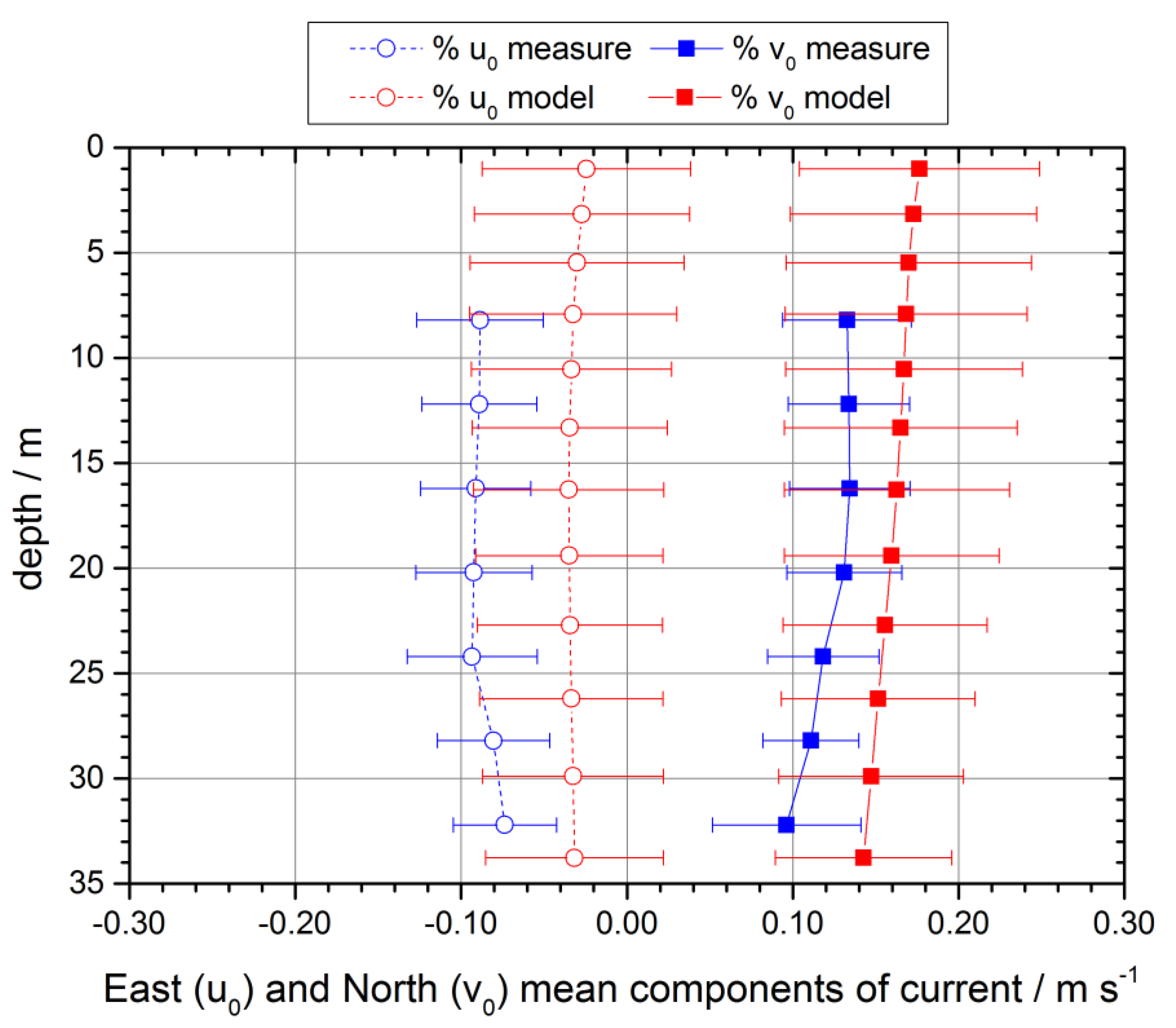
In Figure 16 East and North mean monthly current profiles are reported, showing a reasonable agreement especially with regard to the north components. On the other hand, minor discrepancies appear in relation to the profiles of the east components, closer to positive values in the case of the CMEMS model. Values are however comparable within the limits of the dispersion bands (calculated as standard deviation of measure dispersions in the considered period). A strong barotropic behavior is evident for both components of the model, result of the application of the computational algorithms.

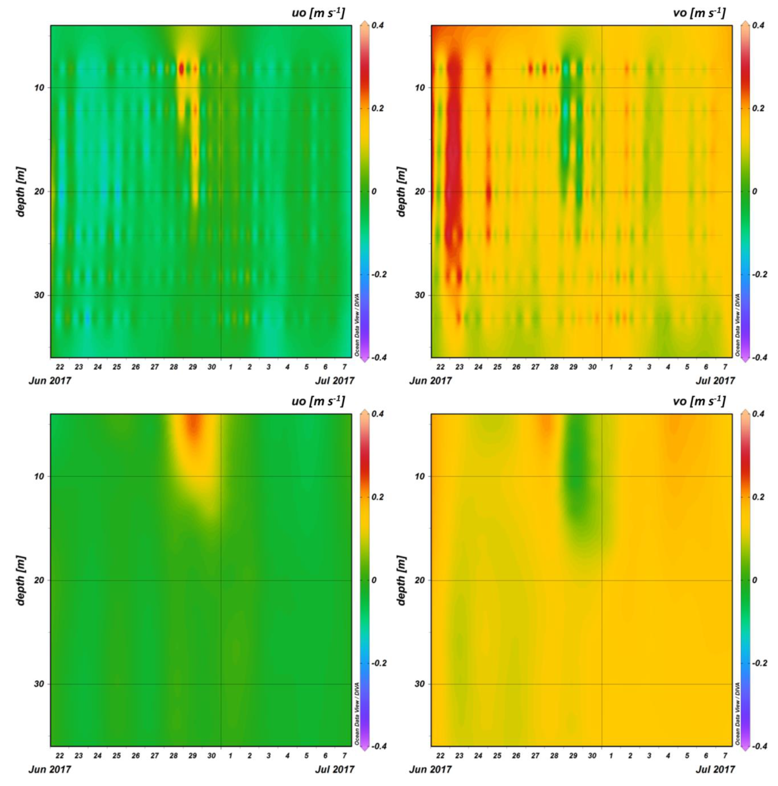
In order to evaluate the differences found between experimental and model data, we focus on a significant phenomenological event, to highlight whether there is congruence between CMEMS outputs at higher temporal resolution and experimental data. Hourly data from the model were then compared with the measurements carried out every 30 min by the ADCP at the end of June 2017, when a significant increase in the East current component and a simultaneous reduction in the North component occurred. Results are reported in Figure 17, showing how CMEMS forecast was able to correctly identify in space and time the eastward rotation of the currents along the water column. On the contrary, the model does not represent well the significant increase in the northern component, clearly noted by the ADCP around the 23 June 2017.

Comparisons with historical data and numerical models need to be supported by a proper uncertainty analysis (section C in [9]). If on one hand the standard uncertainty associated to the heading correction can be calculated by applying the law of uncertainty propagation [19], on the other the spherical law of cosines used to calculate the buoy apparent current is clearly a nonlinear model: therefore, due to correction for buoy apparent currents, standard uncertainties of both net current velocities and their directions need to be calculated in accordance to Monte Carlo method [20], as a by-product of the propagation of the normal probability distributions modeling buoy latitude and longitude values (i.e., the input quantities by which buoy bearing and displacement, and consequently its velocity, are derived).

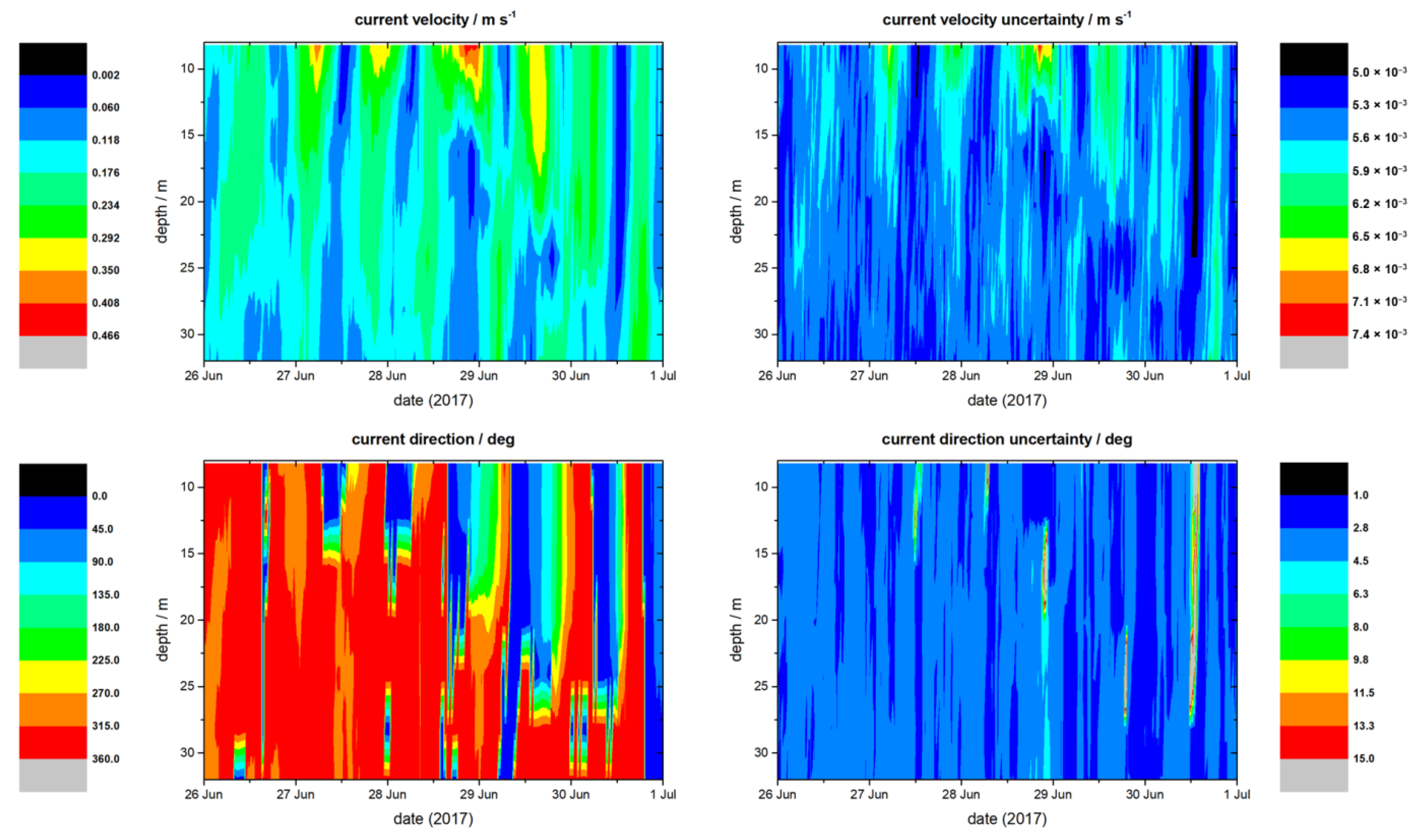
As an applicative example, evaluation of standard uncertainties associated with corrected current velocities is finally reported in Figure 18, computed over the same reference period of Figure 17. This simulation was performed by R software [21], randomly generating M = 10⁶ data for each input quantities.

5. Conclusions

In oceanography, current measurements mostly rely on current profilers, but metrological controls are still missing or poorly applied.

The procedure here described allows a proper uncertainty analysis to be applied on current meters profilers installed on spar buoys. Both the magnetic influence (exerted by the buoy body on the ADCP compass) and the displacement of the buoy itself (origin of apparent currents detectable by the ADCP) are taken into account to assess the measurement reliability. Both heading error and apparent currents can be actually corrected by measuring buoy heading and GPS position

One of the main conclusion is that a standard correction factor could not be applied for every spar buoy equipped with an ADCP, as the effects are case sensitive. The W1-M3A buoy showed to have its own behavior and errors are different for different buoy orientations. The only calibration of the compass is not sufficient to have reliable current measurements from a spar buoy as effects as apparent currents need to be taken into account (and their correction is not linear).

The application of this methodology is also important in order to define an appropriate metric for the comparison of in-situ and models data. The comparison with past ADCP measurements and concurrent model results indicates an overall consistency of the ADCP time series with the dynamics of the area, further supporting the good quality of the applied correction.

The improvement of current estimates can be used to properly validate hydrodynamical models and consequently verify their applicability for specific geographical area. It also allowed us to demonstrate a strong qualitative accordance, in time and space, between the experimental data, literature and hourly model data. The estimation of the performance of an ADCP on a mobile platform is also important in the light of future applications on Argo floats where ADCP can be embedded [5].